Coordinated Shared Spectrum Precoding with Distributed CSIT

The utilization of the radio spectrum is internationally regulated by governments, with the aim of providing wireless communication services that can be efficiently protected from harmful interference. Nevertheless, the tremendous spread of wireless services has given rise to a great need for bandwidth, which cannot be satisfied by an exclusivity of spectral allocation. On the other hand, spectrum scarcity, i.e., the phenomenon where the radio spectrum is becoming vastly underutilized, has been discussed in reports, such as the one published by the Federal Communications Commission (FCC) in 2002 [1]. The spotted under-utilization has given rise, in its turn, to the notion of Cognitive Radio (CR), which has been suggested as a promising technology in view of increasing wireless spectral efficiency by exploiting the existing spectrum holes in time, frequency or space [2, 3].

Focusing on the underlay CR approach, a primary network allows the simultaneous use of its spectral resources by a new-coming (unlicensed) secondary network, given the condition that the latter will utilize the available resources in a way that the interference created by a secondary transmitter (TX) towards a primary receiver (RX) is below a threshold predefined by the primary network [4, 5]. Under such a setup, efficient schemes have been proposed, emphasizing on multiple-antenna settings, with the aim of maximizing the information rate of the secondary system, subject to given constraints over the harmful interference suffered by primary terminals [6, 7, 8, 9, 10]. Importantly, in practice, the ability of the secondary TX to acquire global, multi-user Channel State Information (CSI) is unrealistic. At this point, one would suggest an exchange protocol of channel information between TXs. However, such a protocol would introduce exchange imperfections of channel estimates as well as delays, hence, leading to degraded performance of the designed precoding solution. Consequently, an extensive literature has emphasized on designing transmission schemes, that are robust to imperfect CSI or merely requiring local channel knowledge [See [11] and references therein]. In addition, iterative schemes, based on game theory, have been also investigated as a means of avoiding the need for global multi-user CSI exchange, with respect to spectrum sharing scenarios [12, 13, 14].

Yet, standard spectrum sharing approaches for underlay CR systems, merely focus on designing a transmission scheme for the secondary TX, such that the interference received by a primary terminal would not overcome a certain threshold, beyond which a secure primary connection cannot be established. However, standardization bodies have lately focused on the design of Authorized or Licensed Shared Access systems (termed as ASA and LSA) [15], [16]. The key difference between the latter systems and underlay CR systems is that the incumbents (equivalent to primary nodes in a CR system) can share the spectrum with the licensees (the licensed equivalent of secondary nodes in a CR system), provided that Quality-of-Service (QoS) metrics, that have been negotiated prior to licensing, are satisfied for all involved entities. Motivated by this new framework, it is evident that a major drawback of standard, interference temperature-based underlay CR systems consists in the lack of coordination between the primary and the secondary systems. As a result, in such a way, the primary system tends to overspend its available resources, leading to poor throughput performance at the secondary side.

Given this situation, in this work, we propose the design of a coordination scheme for the two TXs, based on commonly available, slow-varying statistical information. The goal of such a design will be the maximization of the (average) information rate of the licensee system, given that the achievable (average) rate of the incumbent system lies above a certain threshold. More precisely, according to this scheme, the incumbent TX exploits its locally available CSI and the statistical (covariance) information of the global multi-user channel to coordinate with the licensee TX, in order to guarantee the desired average throughput for its assigned terminal. Each TX has access to the instantaneous direct links of its assigned users (as well as their statistics), whereas, the interference cross-links are just statistically known at both TXs. The availability of different estimates of the global downlink channel falls within the paradigm of Team Decision theory, because both transmitters (incumbent and licensee) are actively engaged in cooperation, while being constrained by the locality of the available instantaneous CSI [17, 18, 19, 20, 21].

In [22], a similar scenario was investigated for a single-user underlay CR setup, in the existence of spatially uncorrelated direct channel links, while, in the present work, we focus on the performance of an extended set of applicable joint precoding schemes, with the assumption of correlated Rayleigh fading for all the involved MISO channels. More particularly, our contributions are the following:

• •

  We design a low complexity, statistically coordinated precoding scheme for a MISO spectrum sharing system, which can be applicable to a shared spectrum access system (ASA or LSA). The goal of this design is the maximization of the throughput of the licensee network, in terms of the achievable average rate, given a QoS constraint on the average rate of the incumbent.

• •

  In order to design this joint precoding scheme, we derive lower bounds for the average rate of each RX, in closed form, both when a precoding solution based on Matched Filtering (MF) and statistical Zero-Forcing (sZF), is applied. This way, since the original optimization problem is hard to solve, because of the existence of combined instantaneous and statistical CSI at each of the two TXs, we focus on an approximated version of it.

• •

  Focusing on the approximated version of the optimization problem, we design a set of applicable, joint precoding solutions, the elements of which are joint transmission schemes based on MF or sZF-based beamforming solutions.

• •

  For each of the joint transmission schemes that belong to the referred set, a power policy coordination criterion, which is based on the statistics of the global downlink channel, is applied, with the aim of finding the average transmit power levels at each TX. These power levels are such that the average rate criterion on the incumbent RX is satisfied. Then, the joint beamforming and power allocation scheme that maximizes the average throughput of the licensee RX is selected for transmission. Since such a decision relies on commonly available statistical information, it is taken by both TXs coherently.

• •

  The novel, coordinated precoding scheme is numerically evaluated in comparison to the standard interference temperature-based underlay CR approach. It is shown that our scheme outperforms the standard underlay CR one in a range of system scenarios, which makes our designed precoding policy appealing for LSA systems, since higher average throughput is achieved for the (candidate) licensee system.

Throughout the paper, the following notations are adopted: all boldface letters indicate vectors (lower case) or matrices (upper case). ${\mathbf{A}}^{{{\mathrm{H}}}}$, ${\text{tr}}(\mathbf{A})$ and ${[\mathbf{A}]}_{m,n}$ denote the Hermitian transpose of matrix $\mathbf{A}$, its trace, and its $(m,n)$-th entry, respectively, whereas $\lambda_{j}(\mathbf{A})$ stands for its $j$-th eigenvalue. Also, $\diag\left(\alpha_{1},\ldots,\alpha_{n}\right)$ symbolizes a diagonal matrix, the elements of which are $\alpha_{1},\ldots,\alpha_{n}$. Additionally, $\mathbb{E}[\cdot]$ symbolizes the expectation operator and $\|\cdot\|$ denotes the Euclidean norm, while $\bm{0}_{n}$ denotes the all-zero vector of dimension $n$. The identity matrix of dimension $n\times n$ is denoted by $\mathbf{I}_{n}$, while $\bar{i}$ denotes the complementary index of $i$, when the cardinality of the considered set is equal to two, i.e., $\bar{i}=i$ mod $2+1$. The phase angle between two vectors $\bm{a}$ and $\bm{b}$ is denoted as

$a,b$ and it is defined as: $\vbox to6.94444pt{\hbox{\begin{picture}\put(0.0,0.0){\circle*{0.4}}\put(0.0,0.0){\line{1}{0}{19.51268}}\put(0.0,0.0){\line{1}{2}{5.19792}}\put(5.19792,1.5){\raise 1.94444pt\vbox{\hbox{$\textstyle\bm{a},\bm{b}$}}}\end{picture}}\vss}=\cos^{-1}\left(\frac{\bm{a}^{H}\bm{b}}{\|\bm{a}\|\|\bm{b}\|}\right)$, where $\cos^{-1}(\cdot)$ stands for the inverse cosine function. For a random vector $\bm{x}$, $\bm{x}\sim\mathcal{CN}(\bm{\mu},\mathbf{\Sigma})$ denotes that $\bm{x}$ follows a Circularly Symmetric Complex Gaussian (CSCG) distribution with mean $\bm{\mu}$ and covariance matrix $\mathbf{\Sigma}$. Finally, $E_{1}(\cdot)$ represents the exponential integral function, which is defined in [23, eq. (5.1.1)], while $\gamma\approx 0.5772$ stands for the Euler-Mascheroni constant, as it is defined in [23, eq. (4.1.32)].

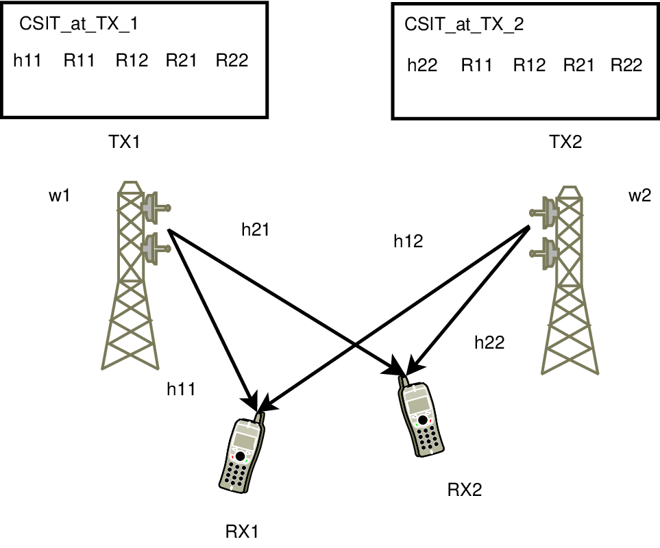
The spectrum sharing system, which is illustrated in Fig. 1, is composed of a MISO incumbent system, comprising of a TX, ${\textrm{TX}}~1$, equipped with $M_{1}$ antennas, along with its assigned single-antenna terminal, ${\textrm{RX}}~1$. Focusing on downlink communication, the incumbent system is willing to share its resources with a MISO licensee system. The latter system consists of a multiple antenna TX, ${\textrm{TX}}~2$, equipped with $M_{2}$ antennas, as well as of a licensee terminal, ${\textrm{RX}}~2$, assigned to ${\textrm{TX}}~2$.

Considering the involved channels, spatially correlated Rayleigh fading is assumed for both direct and interfering channel links. As a consequence, for the channel between ${\textrm{TX}}~j$ and ${\textrm{RX}}~i$, we have: $\bm{h}_{i,j}\sim\mathcal{CN}(\bm{0}_{M_{j}},\mathbf{R}_{i,j})$.

The signal received at ${\textrm{RX}}~i,\hskip 7.22743pti\in\{1,2\}$, can be expressed as

$$y_{i}=\bm{h}_{i,i}^{{{\mathrm{H}}}}\bm{w}_{i}s_{i}+\bm{h}_{i,\bar{i}}^{{{\mathrm{H}}}}\bm{w}_{\bar{i}}s_{\bar{i}}+n_{i},$$

(1)

where, $\bm{w}_{i}$ denotes the transmit beamforming vector at ${\textrm{TX}}~i$ and it is assumed that $\bm{w}_{i}=\sqrt{P_{i}}\bm{u}_{i}$, with $P_{i}\leq P_{i}^{\max}$ and $\|\bm{u}_{i}\|=1$, where $P_{i}^{\max}$ is a maximum instantaneous power level at ${\textrm{TX}}~i$. Also, Gaussian noise is considered at ${\textrm{RX}}~i$, i.e., $n_{i}\sim\mathcal{CN}(0,N_{0})$ and we assume that the information symbols for transmission are taken from a standard complex Gaussian codebook, i.e., $s_{i}\sim\mathcal{CN}(0,1),\hskip 7.22743pti\in\{1,2\}$. By analyzing (1), the instantaneous information rate of ${\textrm{RX}}~i,\hskip 7.22743pti\in\{1,2\}$ is given by [24]

$$R_{i}=\log_{2}\Bigg(1+\frac{P_{i}{|\bm{h}_{i,i}^{{{\mathrm{H}}}}\bm{u}_{i}|}^{2}}{N_{0}+P_{\bar{i}}{|\bm{h}_{i,\bar{i}}^{{{\mathrm{H}}}}\bm{u}_{\bar{i}}|}^{2}}\Bigg).$$

(2)

In the section that follows, the problem of joint downlink precoding with combined, local CSI at the TX (CSIT), is formulated.

Focusing on the described system model, a realistic CSIT assumption that can be made is that ${\textrm{TX}}~i,\hskip 7.22743pti\in\{1,2\}$, has both instantaneous and statistical (covariance) knowledge of its direct links (i.e., ${\textrm{TX}}~1$ has instantaneous knowledge of direct link $\bm{h}_{1,1}$ and ${\textrm{TX}}~2$ has instantaneous knowledge of direct link $\bm{h}_{2,2}$), whereas, the interference cross-links are merely statistically known via knowledge of their covariance matrices. The second order statistics of the involved channels constitute slow-varying information that can be realistically collected by each TX through low capacity/high delay links.

Capitalizing on the available CSIT at ${\textrm{TX}}~i,\hskip 7.22743pti\in\{1,2\}$, the optimization problem of maximizing the average rate of the licensee system, subject to an average rate constraint for ${\textrm{RX}}~1$ can be formulated as a functional optimization problem, with functional dependencies related to the available CSI. Hence, the resulting optimization problem can be described as follows

		$\displaystyle\big(\bm{w}_{1}^{*},\bm{w}_{2}^{*}\big)=\arg\max{\mathbb{E}}\left[R_{2}\left(\bm{w}_{1}(\bm{h}_{1,1}),\bm{w}_{2}(\bm{h}_{2,2})\right)\right]$		(P1)
		$\displaystyle{\displaystyle\textrm{subject}}\hskip 7.22743pt{\textrm{to}}\hskip 7.22743pt{\mathbb{E}}\left[R_{1}\left(\bm{w}_{1}(\bm{h}_{1,1}),\bm{w}_{2}(\bm{h}_{2,2})\right)\right]\geq\tau_{1}>0,$
		$\displaystyle 0\leq{\|\bm{w}_{1}(\bm{h}_{1,1})\|}^{2}\leq P_{1}^{\max},\hskip 7.22743pt0\leq{\|\bm{w}_{2}(\bm{h}_{2,2})\|}^{2}\leq P_{2}^{\max},$

where $\tau_{1}$ stands for the QoS demand of $\textrm{RX}~1$, in terms of average rate.

The dependencies of the precoders to be optimized, on the corresponding instantaneous links, can be formulated by the following mappings

	$\displaystyle\bm{w}_{i}:\hskip 7.22743pt\mathbb{C}^{M_{i}}$	$\displaystyle\rightarrow\mathbb{C}^{M_{i}}$		(3)
	$\displaystyle\bm{h}_{i,i}$	$\displaystyle\mapsto\bm{w}_{i}(\bm{h}_{i,i}),$

where $i\in\{1,2\}$. Hence, the formulated optimization problem is of distributed nature. In what follows, for ease of exposition, we will omit to mention explicitly the dependencies of the precoders.

One has to ensure that problem (P1) is feasible, in other words, QoS threshold $\tau_{1}$ has to be achievable when ${\textrm{TX}}~1$ transmits with full power MF precoding, in the absence of any interference coming from the licensee. This means satisfying the following

$$\mathbb{E}\left[\log_{2}\bigg(1+\frac{P_{1}^{\max}\|\bm{h}_{1,1}\|^{2}}{N_{0}}\bigg)\right]\geq\tau_{1}.$$

(4)

The expectation over the interfering channels makes the optimization difficult to handle. However, exploiting the convexity of function $\log_{2}\left(1+\frac{1}{x}\right)$, it becomes possible to apply Jensen’s inequality [24] over the interfering channels. This significantly simplifies the optimization problem, while preserving its important features. The average rate expression for RX $i$, thus, becomes

	$\displaystyle{\mathbb{E}}\left[R_{i}\right]$	$\displaystyle={\mathbb{E}}_{\bm{h}_{i,i},\bm{h}_{i,\bar{i}}}\left[\log_{2}\left(1+\frac{P_{i}{|\bm{h}_{i,i}^{{{\mathrm{H}}}}\bm{u}_{i}|}^{2}}{N_{0}+P_{\bar{i}}{|\bm{h}_{i,\bar{i}}^{{{\mathrm{H}}}}\bm{u}_{\bar{i}}|}^{2}}\right)\right]$		(5)
		$\displaystyle\geq{\mathbb{E}}_{\bm{h}_{i,i}}\left[\log_{2}\left(1+\frac{P_{i}{|\bm{h}_{i,i}^{{{\mathrm{H}}}}\bm{u}_{i}|}^{2}}{N_{0}+{\mathbb{E}}_{\bm{h}_{i,\bar{i}}}\left[P_{\bar{i}}{|\bm{h}_{i,\bar{i}}^{{{\mathrm{H}}}}\bm{u}_{\bar{i}}|}^{2}\right]}\right)\right]$
		$\displaystyle={\mathbb{E}}_{\bm{h}_{i,i}}\left[\log_{2}\left(1+\frac{P_{i}{|\bm{h}_{i,i}^{{{\mathrm{H}}}}\bm{u}_{i}|}^{2}}{N_{0}+P_{\bar{i}}\bm{u}_{\bar{i}}^{{{\mathrm{H}}}}\mathbf{R}_{i,\bar{i}}\bm{u}_{\bar{i}}}\right)\right]$
		$\displaystyle\triangleq{\mathbb{E}}\left[\tilde{R}_{i}(\bm{w}_{i},\bm{w}_{\bar{i}})\right].$

With the aim of deriving a practical solution, slow power control depending on the long term statistical channel information, is assumed. Hence, instead of (instantaneous) power levels $P_{1}$ and $P_{2}$, we can use slow power allocation levels $\bar{P}_{1}$ and $\bar{P}_{2}$, where $0\leq\bar{P}_{i}\leq P_{i}^{\max},\hskip 7.22743pti\in\{1,2\}$.

Altogether, in the remainder of the paper, we will work on the following optimization problem:

		$\displaystyle(\bar{P}_{1}^{*},\bm{u}_{1}^{*},\bar{P}_{2}^{*},\bm{u}_{2}^{*})=\arg\max~~{\mathbb{E}}\left[\tilde{R}_{2}(\bar{P}_{1},\bm{u}_{1},\bar{P}_{2},\bm{u}_{2})\right]$		(P2)
		$\displaystyle{\displaystyle\textrm{subject}}\hskip 7.22743pt{\textrm{to}}\hskip 7.22743pt{\mathbb{E}}\left[\tilde{R}_{1}(\bar{P}_{1},\bm{u}_{1},\bar{P}_{2},\bm{u}_{2})\right]\geq\tau_{1},$
		$\displaystyle 0\leq\bar{P}_{1}\leq P_{1}^{\max},\hskip 7.22743pt0\leq\bar{P}_{2}\leq P_{2}^{\max},$
		$\displaystyle\|\bm{u}_{1}\|=1,\hskip 7.22743pt\|\bm{u}_{2}\|=1.$

The following two propositions provide some characteristics of the optimal solution of problem (P2).

The second proposition yields some insight with respect to the optimal power allocation scheme.

We now present our main contribution which is a new transmission scheme constituting a possible solution for optimization problem (P1). Indeed, it is important to note that, although possibly suboptimal, our approach is able to guarantee the incumbent rate constraint and is, therefore, a solution to the initial optimization problem.

In this section, we present two schemes which will be used to evaluate the efficiency of our statistically coordinated precoding approach.

The first one, denoted as “interference temperature-based” precoding, is an adaptation of the approaches in the literature to allow for a fair comparison. Intuitively, it corresponds to the conventional underlay CR paradigm, where solely the secondary TX adapts its strategy in order for the interference received by the primary RX to be below a given threshold [5].

The second one constitutes a coordination benchmark and it is a priori not reachable, but allows to bound the sub-optimality of the proposed approach.

With the aim of evaluating the performance of the proposed statistically coordinated precoding scheme, extensive Monte Carlo simulations have been performed and, more specifically, $20000$ channel realizations have been simulated. We assume the existence of $M_{1}=M_{2}=M=4$ antennas at each TX. Furthermore, we consider unit noise variance ($N_{0}=1$) and a QoS threshold $\tau_{1}=1$ bps/Hz.

We consider a classical exponential channel correlation model [25], in which the covariance matrices $\mathbf{R}_{i,j}$ are given by

$$\mathbf{R}_{i,j}=\beta_{i,j}\begin{bmatrix}1&\rho&\rho^{2}&\ldots&\rho^{M-1}\\ \rho&1&\rho&\ldots&\rho^{M-2}\\ \vdots&\vdots&\vdots&\ddots&\vdots\\ \rho^{M-1}&\rho^{M-2}&\rho^{M-3}&\ldots&1\\ \end{bmatrix},\hskip 7.22743pti,j\in\{1,2\},$$

(18)

where, $\beta_{i,j}$ represents the pathloss and is chosen here equal to $1$ when $i=j$ and to $0.3$ otherwise. In the investigated scenario the antenna correlation factor, $\rho$, is equal to 0.5.

In Fig. 2 and Fig. 3, the average rate of RX $1$ and the average rate of ${\textrm{RX}}~2$ are depicted as a function of the system’s transmit Signal-to-Noise Ratio (SNR). The three curves represent the throughput performance achieved by the proposed statistically coordinated precoding scheme, the interference temperature-based precoding scheme, as well as the described coordination benchmark. Focusing on RX $2$, the coordination benchmark outperforms both the proposed precoding scheme as well as the interference temperature-based scheme, as expected. By observing Fig. 2, it should be noted that, in contrast with the coordination benchmark, the proposed precoding scheme fails to satisfy the incumbent average rate constraint with equality. This occurs because we resort to tackling optimization problem (P2), which involves a lower bound of the average rate of RX $1$. Nevertheless, the proposed algorithm successfully manages to control the average rate of RX $1$ and this capability can be translated to a significant throughput gain for the licensee, in comparison to the one achieved by the interference temperature-based precoding scheme.

The achievable average rates of RX $1$ and RX $2$, by applying the proposed precoding algorithm, along with the ones achieved by the two reference precoding schemes, are depicted in Fig. 4 and Fig. 5, respectively, as a function of QoS threshold, $\tau_{1}$, when the transmit SNR of the system is equal to $10$ dB. The average rate constraint for RX $1$ is fulfilled by all three schemes for the whole examined range of $\tau_{1}$. Also, the proposed precoding scheme outperforms the interference temperature-based one, especially when the average rate constraint of the incumbent is loose, which occurs due to the fact that under this regime there is more to gain for the licensee by means of an efficient coordination.

In this work, we propose a novel, joint precoding scheme with reference to a shared spectrum access system where the two TXs coordinate on the basis of statistical knowledge of the global multi-user channel. Our approach consists in formulating a Team Decision problem, the solution of which is approached by reducing the transmission strategy space to a finite number of strategies. This method is key to enforcing between the TXs and obtaining a practical solution to the intricate Team Decision problem. Such an approach allows to improve over the conventional underlay CR approach, by enforcing more coordination between the two coexisting TXs at the price of low CSI and complexity requirements, as the coordination can be realized offline. Approaching the global optimum is both a difficult and challenging problem that can be tackled in the future. The proposed scheme has also a strong potential in other more complex scenarios with multiple incumbent and/or licensee networks.

References

- [1] Federal Communications Commission, “Spectrum policy task force report, FCC 02-155,” 2002.
- [2] J. Mitola and J. Maguire, G.Q., “Cognitive radio: making software radios more personal,” IEEE Personal Communications, vol. 6, no. 4, pp. 13–18, Aug. 1999.
- [3] S. Haykin, “Cognitive radio: brain-empowered wireless communications,” IEEE Journal on Selected Areas in Communications, vol. 23, no. 2, pp. 201–220, Feb. 2005.
- [4] A. Goldsmith, S. Jafar, I. Maric, and S. Srinivasa, “Breaking spectrum gridlock with cognitive radios: An information theoretic perspective,” Proceedings of the IEEE, vol. 97, no. 5, pp. 894–914, May 2009.
- [5] E. Biglieri, A. J. Goldsmith, L. J. Greenstein, N. Mandayam, and H. V. Poor, Principles of Cognitive Radio. Cambridge University Press, 2012.
- [6] R. Zhang and Y.-C. Liang, “Exploiting multi-antennas for opportunistic spectrum sharing in cognitive radio networks,” IEEE Journal of Selected Topics in Signal Processing, vol. 2, no. 1, pp. 88–102, Feb. 2008.
- [7] S.-J. Kim and G. Giannakis, “Optimal resource allocation for MIMO ad hoc cognitive radio networks,” IEEE Transactions on Information Theory, vol. 57, no. 5, pp. 3117–3131, May 2011.
- [8] R. Zhang, “On peak versus average interference power constraints for protecting primary users in cognitive radio networks,” IEEE Transactions on Wireless Communications, vol. 8, no. 4, pp. 2112–2120, Apr. 2009.
- [9] Y. Huang and D. Palomar, “Rank-constrained separable semidefinite programming with applications to optimal beamforming,” IEEE Transactions on Signal Processing, vol. 58, no. 2, pp. 664–678, Feb. 2010.
- [10] L. B. Le and E. Hossain, “Resource allocation for spectrum underlay in cognitive radio networks,” IEEE Transactions on Wireless Communications, vol. 7, no. 12, pp. 5306–5315, Dec. 2008.
- [11] K.-Y. Wang, N. Jacklin, Z. Ding, and C.-Y. Chi, “Robust MISO transmit optimization under outage-based QoS constraints in two-tier heterogeneous networks,” IEEE Transactions on Wireless Communications, vol. 12, no. 4, pp. 1883–1897, Apr. 2013.
- [12] B. Wang, Y. Wu, and K. R. Liu, “Game theory for cognitive radio networks: An overview,” Computer Networks, vol. 54, no. 14, pp. 2537 – 2561, 2010.
- [13] G. Scutari and D. Palomar, “MIMO cognitive radio: A game theoretical approach,” IEEE Transactions on Signal Processing, vol. 58, no. 2, pp. 761–780, Feb. 2010.
- [14] W. Zhong, Y. Xu, and H. Tianfield, “Game-theoretic opportunistic spectrum sharing strategy selection for cognitive MIMO multiple access channels,” IEEE Transactions on Signal Processing, vol. 59, no. 6, pp. 2745–2759, Jun. 2011.
- [15] E. CEPT, “Licensed shared access (LSA),” ECC Report, vol. 205, 2014.
- [16] J. Holdren and E. Lander, “Realizing the full potential of government-held spectrum to spur economic growth,” Technical Report, Tech. Rep., 2012.
- [17] R. Radner, “Team decision problems,” The Annals of Mathematical Statistics, vol. 33, no. 3, pp. pp. 857–881, 1962.
- [18] Y.-C. Ho, “Team decision theory and information structures,” Proceedings of the IEEE, vol. 68, no. 6, pp. 644–654, 1980.
- [19] R. Zakhour and D. Gesbert, “Team decision for the cooperative MIMO channel with imperfect CSIT sharing,” in Information Theory and Applications Workshop (ITA), 2010, Jan. 2010, pp. 1–6.
- [20] P. de Kerret and D. Gesbert, “CSI sharing strategies for transmitter cooperation in wireless networks,” IEEE Wireless Communications, vol. 20, no. 1, pp. 43–49, Feb. 2013.
- [21] M. C. Filippou, G. A. Ropokis, and D. Gesbert, “A team decisional beamforming approach for underlay cognitive radio networks,” in IEEE 24th International Symposium on Personal Indoor and Mobile Radio Communications (PIMRC), 2013, Sep. 2013, pp. 575–579.
- [22] P. de Kerret, M. Filippou, and D. Gesbert, “Statistically coordinated precoding for the MISO cognitive radio channel,” in 48th Asilomar Conference on Signals, Systems and Computers, 2014, Nov. 2014, pp. 1083–1087.
- [23] M. Abramowitz and I. A. Stegun, Handbook of mathematical functions. Dover publications, 1965.
- [24] T. M. Cover and J. A. Thomas, Elements of information theory. John Wiley & Sons, 2012.
- [25] S. Loyka, “Channel capacity of MIMO architecture using the exponential correlation matrix,” IEEE Communications Letters, vol. 5, no. 9, pp. 369–371, Sep. 2001.
- [26] R. Mallik, M. Win, J. Shao, M.-S. Alouini, and A. Goldsmith, “Channel capacity of adaptive transmission with maximal ratio combining in correlated Rayleigh fading,” IEEE Transactions on Wireless Communications, vol. 3, no. 4, pp. 1124–1133, Jul. 2004.
- [27] J. Wang, S. Jin, X. Gao, K.-K. Wong, and E. Au, “Statistical eigenmode-based SDMA for two-user downlink,” IEEE Transactions on Signal Processing, vol. 60, no. 10, pp. 5371–5383, Oct. 2012.
- [28] E. Abbe, S.-L. Huang, and E. Telatar, “Proof of the outage probability conjecture for MISO channels,” in 2012 IEEE Information Theory Workshop (ITW), Sep. 2012, pp. 65–69.
- [29] I. S. Gradshteyn and I. M. Ryzhik, Table of integrals, series, and products, 7th ed. Elsevier/Academic Press, Amsterdam, 2007.