Second-Order Region for Gray-Wyner Network

Shun Watanabe ^†^†thanks: S.˜Watanabe is with the Department of Computer and Information Sciences, Tokyo University of Agriculture and Technology, Japan, E-mail:shunwata@cc.tuat.ac.jp.

Abstract

The coding problem over the Gray-Wyner network is studied from the second-order coding rates perspective. A tilted information density for this network is introduced in the spirit of Kostina-Verdú, and, under a certain regularity condition, the second-order region is characterized in terms of the variance of this tilted information density and the tangent vector of the first-order region. The second-order region is proved by the type method: the achievability part is proved by the type-covering argument, and the converse part is proved by a refinement of the perturbation approach that was used by Gu-Effros to show the strong converse of the Gray-Wyner network. This is the first instance that the second-order region is characterized for a multi-terminal problem where the characterization of the first-order region involves an auxiliary random variable.

I Introduction

We study the coding problem over the Gray-Wyner network [6] from the second-order coding rates perspective. The study of the second-order coding rates has attracted significant interest in recent years since it gives a good approximation for the finite blocklength performance of certain coding systems [10, 25]. The second-order coding rates for point-to-point systems are quite well-understood [29, 10, 25, 9, 19, 23, 16, 13, 17, 35, 18, 36]. On the other hand, the extension of the second-order analysis to multi-terminal problems is rather immature; some problems are solved completely [31, 24, 32, 20, 28, 11, 34, 33], but only achievability bounds are known for other problems [31, 21, 12, 27, 37, 39, 26]. See [30] for further review of existing results on the second-order analysis.

The Gray-Wyner network is described in Fig. 1. The network consists of one encoder and two decoders. The encoder and both the decoders are connected by the common channel, and each decoder is also connected to the encoder by its own private channel. Then, the goal for each decoder is to almost losslessly reproduce one part of correlated sources, and we are interested in the optimal trade-off among the rates of the three channels. The information theoretic chanracterization of achievable rate triplets was derived in [6], and, as is typical for multi-terminal problems (cf. [5]), it involves an auxiliary random variable, which makes the second-order analysis of this problem non-trivial.

I-A Contributions

We characterize the second-order region of the Gray-Wyner network under a certain regularity condition.¹¹ 1 Because of the regularity condition, our result cannot be applied to singular points on the boundary of the first-order region, i.e., the boundary points where the first-order region cannot be differentiated. For that purpose, we introduce a tilted information density for this network in the spirit of Kostina-Verdú [16]. Then, the second-order region is characterized in terms of the variance of this tilted information density and the tangent vector of the first-order region. Since the first-order region of the Gray-Wyner network is characterized by an auxiliary random variable, the tilted information density is defined by using that auxiliary random variable. In general, there is no guarantee that an optimal test channel is unique, and more than one optimal test channel may exist. However, we show that the tilted information density is uniquely defined irrespective of the choice of optimal test channels. Also, we show some other properties of the tilted information density.

In [6], the plane where the sum of the three rates coincide with the joint entropy of the correlated sources was called the Pangloss plane, and it gained a special attention since there is no sum-rate loss compared to cooperative decoding schemes on this plane. When the first-order rates are on the Pangloss plane, as an illustration of our main result, we show a simple expression of the second-order region. Interestingly, the sum constraint of the second-order rates coincide with that can be achieved by cooperative decoding schemes; this means that there is no sum-rate loss compared to cooperative decoding schemes even up to the second-order.

In the proof of the second-order region, we use the type method. The achievability part is proved by an application of the type covering argument (cf. [40] and [4, Chapter 9]). For the converse part, we refine the perturbation approach that was used by Gu-Effros [7, 8] to show the strong converse of the Gray-Wyner network. By these argument, we first derive an upper bound and a lower bound on the error probability in terms of a probability of a certain function of the joint type. Then, we approximate that probability by using the central limit theorem.

When we use the type method for the second-order analysis, say the rate-distortion problem, we take a derivative of the rate-distortion function with respect to the source distribution, and the second-order rate is characterized in terms of the variance of that derivative (cf. [13]). Then, we can show that that characterization coincides with the variance of the $d$ -tilted information introduced in [16]. In this paper, we consider a slightly different argument. When we take a derivative of a certain function of a distribution, we have to extend the domain of that function to the outside of the probability simplex (cf. [22, Appendix A]). In order to circumvent such an extension, we consider a different parameterization of the probability simplex, which is often used in information geometry [1]. Then, we take a derivative of the function with respect to that parameter. Also, instead of introducing the variance of the derivative, we directly characterize the second-order region in terms of the variance of the tilted information density.

I-B Paper Organization

The rest of the paper is organised as follows: In Section II, we introduce our notation, and recall the problem formulation of the Gray-Wyner network. In Section III, we introduce the tilted information density for the Gray-Wyner network, and investigate its properties. Then, in Section IV, we show our second-order coding theorem and its proof. In Section V, we further investigate the Pangloss plane. We conclude the paper with some discussions in Section VI.

Refer to caption — Fig. 1: A description of the Gray-Wyner network.

II Problem Formulation

In this section, we introduce our notations and recall the Gray-Wyner network [6].

II-A Notations

Random variables (e.g. $X$ ) and their realizations (e.g. $x$ ) are in capital and lower case, respectively. All random variables take values in some finite alphabets which are denoted in calligraphic font (e.g. ${\cal X}$ ). The cardinality of ${\cal X}$ is denoted as $|{\cal X}|$ . Let the random vector $X^{n}=(X_{1},\ldots,X_{n})$ and similarly for a realization $\bm{x}=(x_{1},\ldots,x_{n})$ . For information theoretic quantities, we follows the same notations as [4]; e.g. the entropy and the mutual information are denoted by $H(X)$ and $I(X\wedge Y)$ , respectively. Also, the expectation and the variance are denoted by $\mathsf{E}[\cdot]$ and $\mathsf{V}[\cdot]$ respectively. $\mathsf{Q}(t)=\int_{t}^{\infty}\frac{1}{\sqrt{2\pi}}e^{-\frac{u^{2}}{2}}du$ is the upper tail probability of the standard normal distribution; its inverse is denoted by $\mathsf{Q}^{-1}(\varepsilon)$ for $0<\varepsilon<1$ .

The set of all distribution on ${\cal X}$ is denoted by ${\cal P}({\cal X})$ . The set of all channels from ${\cal X}$ to ${\cal Y}$ is denoted by ${\cal P}({\cal Y}|{\cal X})$ . We will also use the method of types [4]. For a given sequence $\bm{x}$ , its type is denoted by $\mathsf{t}_{\bm{x}}$ . The set of all types on ${\cal X}$ is denoted by ${\cal P}_{n}({\cal X})$ , and the set of all conditional types is denoted by ${\cal P}_{n}({\cal Y}|{\cal X})$ . For a given type $P_{\bar{X}}\in{\cal P}_{n}({\cal X})$ , the set of all sequences with type $P_{\bar{X}}$ is denoted by ${\cal T}_{\bar{X}}^{n}$ . For a given joint type $P_{\bar{X}\bar{Y}}$ and a sequence $\bm{x}\in{\cal T}_{\bar{X}}^{n}$ , the set of all sequences whose joint type with $\bm{x}$ is $P_{\bar{X}\bar{Y}}$ is denoted by ${\cal T}_{\bar{Y}|\bar{X}}^{n}(\bm{x})$ . For type $P_{\bar{X}}$ and joint type $P_{\bar{X}\bar{Y}}$ , we use notations $H(\bar{X})$ and $I(\bar{X}\wedge\bar{Y})$ , where the random variables are distributed according to those type and joint type.

For a given distribution $P_{X}$ , its support is denoted by $\mathtt{supp}(P_{X})$ . In latter sections, we will differentiate a certain function of distributions around a given joint distribution $P_{XY}$ , which may not have full support. For that purpose, it is convenient to introduce a parametrization for distribution $P$ that has the same support as $P_{XY}$ .²² 2 In the literature [13] (see also [22]), the probability simplex is embedded into the Euclidian space, and the parameterization on that Euclidian space is used. However in this paper, we regard the probability simplex as a manifold (cf. [1]), and we consider a parameterization that is different from the literature so that we do not have to extend the domain of a certain function to outside the probability simplex. Let $m=\mathtt{supp}(P_{XY})$ ; without loss of generality, we assign $1$ through $m$ to elements in $\mathtt{supp}(P_{XY})$ . Then, parameter $\theta(P)\in\mathbb{R}^{m-1}$ is defined as $\theta_{i}=P(i)$ for $i=1,\ldots,m-1$ ; apparently it holds $P(m)=1-\sum_{i=1}^{m-1}\theta_{i}$ . The distribution corresponding to parameter $\theta$ is denoted by $P_{\theta}$ .

II-B Gray-Wyner Network

In this section, we recall the lossless source coding problem over the Gray-Wyner network (see Fig. 1). Let us consider a correlated source $(X,Y)$ taking values in ${\cal X}\times{\cal Y}$ and having joint distribution $P_{XY}$ . We consider a block coding of length $n$ . A coding system consists of three encoders

		$\displaystyle\varphi^{(n)}_{0}:{\cal X}^{n}\times{\cal Y}^{n}\to{\cal M}_{0}^{(n)},$		(1)
		$\displaystyle\varphi^{(n)}_{1}:{\cal X}^{n}\times{\cal Y}^{n}\to{\cal M}^{(n)}_{1},$		(2)
		$\displaystyle\varphi^{(n)}_{2}:{\cal X}^{n}\times{\cal Y}^{n}\to{\cal M}^{(n)}_{2},$		(3)

and two decoders

		$\displaystyle\psi^{(n)}_{1}:{\cal M}^{(n)}_{0}\times{\cal M}^{(n)}_{1}\to{\cal X}^{n},$		(4)
		$\displaystyle\psi^{(n)}_{2}:{\cal M}^{(n)}_{0}\times{\cal M}^{(n)}_{2}\to{\cal Y}^{n}.$		(5)

The message encoded by $\varphi^{(n)}_{0}$ is sent over the common channel, and received by both the decoders; the message encoded by $\varphi^{(n)}_{i}$ is sent over the private channel to $i$ th decoder, where $i=1,2$ . The first decoder is required to reproduce $X^{n}$ almost losslessly, while the second decoder is required to reproduce $Y^{n}$ almost losslessly. In the following, we omit the blocklength $n$ when it is obvious from the context. For $(X^{n},Y^{n})\sim P$ , the error probability of code $\Phi_{n}=(\varphi_{0},\varphi_{1},\varphi_{2},\psi_{1},\psi_{2})$ is defined as

\displaystyle\mathrm{P}_{\mathrm{e}}(\Phi_{n}|P):=\Pr\bigg((\psi_{1}(\varphi_{0}(X^{n},Y^{n}),\varphi_{1}(X^{n},Y^{n})),\psi_{2}(\varphi_{0}(X^{n},Y^{n}),\varphi_{2}(X^{n},Y^{n})))\neq(X^{n},Y^{n})\bigg).

(6)

Then, the correct probability of the code is defined as

\displaystyle\mathrm{P}_{\mathrm{c}}(\Phi_{n}|P):=1-\mathrm{P}_{\mathrm{e}}(\Phi_{n}|P).

(7)

In the following, we are particularly interested in the case where $P$ is a product distribution $P_{XY}^{n}$ , i.e., $(X^{n},Y^{n})$ is an i.i.d. sequence.

Definition 1 (First-Order Region)

The rate triplet $(r_{0},r_{1},r_{2})\in\mathbb{R}_{+}^{3}$ is defined to be achievable if there exists a sequence of code $\{\Phi_{n}\}_{n=1}^{\infty}$ such that

$\displaystyle\limsup_{n\to\infty}\frac{1}{n}\log\|{\cal M}_{0}^{(n)}\|$	$\displaystyle\leq r_{0},$	(8)
$\displaystyle\limsup_{n\to\infty}\frac{1}{n}\log\|{\cal M}_{1}^{(n)}\|$	$\displaystyle\leq r_{1},$	(9)
$\displaystyle\limsup_{n\to\infty}\frac{1}{n}\log\|{\cal M}_{2}^{(n)}\|$	$\displaystyle\leq r_{2},$	(10)

and

\displaystyle\lim_{n\to\infty}\mathrm{P}_{\mathrm{e}}(\Phi_{n}|P_{XY}^{n})=0.

(11)

Then, the achievable region ${\cal R}_{\mathtt{GW}}(P_{XY})$ is defined as the set of all achievable rate triplets.

The first-order region ${\cal R}_{\mathtt{GW}}(P_{XY})$ is characterized in [6]. Let ${\cal R}_{\mathtt{GW}}^{*}(P_{XY})$ be the set of all rate triplets $(r_{0},r_{1},r_{2})$ such that there exists a test channel $P_{W|XY}$ with $|{\cal W}|\leq|{\cal X}||{\cal Y}|+2$ such that

$\displaystyle r_{0}$	$\displaystyle\geq I(W\wedge X,Y),$	(12)
$\displaystyle r_{1}$	$\displaystyle\geq H(X\|W),$	(13)
$\displaystyle r_{2}$	$\displaystyle\geq H(Y\|W).$	(14)

Proposition 1 ([6])

It holds that³³ 3 In fact, the cardinality bound was not shown in [6], but it can be proved by the support lemma [4] (see also [14]).

\displaystyle{\cal R}_{\mathtt{GW}}(P_{XY})={\cal R}^{*}_{\mathtt{GW}}(P_{XY}).

(15)

In this paper, we are interested in the second-order region. We follow the second-order formulation in [24].

Definition 2 (Second-Order Region)

For a boundary point $(r_{0}^{*},r_{1}^{*},r_{2}^{*})$ of ${\cal R}_{\mathtt{GW}}(P_{XY})$ and $0<\varepsilon<1$ , the rate triplet $(L_{0},L_{1},L_{2})\in\mathbb{R}^{3}$ is defined to be $(\varepsilon,r_{0}^{*},r_{1}^{*},r_{2}^{*})$ -achievable if there exists a sequence of code $\{\Phi_{n}\}_{n=1}^{\infty}$ such that

$\displaystyle\limsup_{n\to\infty}\frac{\log\|{\cal M}_{0}^{(n)}\|-nr_{0}^{*}}{\sqrt{n}}$	$\displaystyle\leq L_{0},$	(16)
$\displaystyle\limsup_{n\to\infty}\frac{\log\|{\cal M}_{1}^{(n)}\|-nr_{1}^{*}}{\sqrt{n}}$	$\displaystyle\leq L_{1},$	(17)
$\displaystyle\limsup_{n\to\infty}\frac{\log\|{\cal M}_{2}^{(n)}\|-nr_{2}^{*}}{\sqrt{n}}$	$\displaystyle\leq L_{2},$	(18)

and

\displaystyle\limsup_{n\to\infty}\mathrm{P}_{\mathrm{e}}(\Phi_{n}|P_{XY}^{n})\leq\varepsilon.

(19)

Then, the $(\varepsilon,r_{0}^{*},r_{1}^{*},r_{2}^{*})$ -achievable region ${\cal L}_{\mathtt{GW}}(\varepsilon;r_{0}^{*},r_{1}^{*},r_{2}^{*})$ is defined as the set of all $(\varepsilon,r_{0}^{*},r_{1}^{*},r_{2}^{*})$ -achievable rate triplets.

In contrast to first-order rates, second-order rates may be negative even though they are conventionally called “rates”.

III Tilted Information Density

In this section, we introduce the tilted information density for the Gray-Wyner network in the spirit of [16]. The tilted information density plays an important role to characterize the second-order region ${\cal L}_{\mathtt{GW}}(\varepsilon;r_{0}^{*},r_{1}^{*},r_{2}^{*})$ in the next section.

Given $r_{1},r_{2}>0$ , let

	$\displaystyle R(r_{1},r_{2}\|P_{XY})$	$\displaystyle:=\min\big\{r_{0}:(r_{0},r_{1},r_{2})\in{\cal R}_{\mathtt{GW}}^{*}(P_{XY})\big\}$		(20)
		$\displaystyle=\min\big\{I(W\wedge X,Y):\|{\cal W}\|\leq\|{\cal X}\|\|{\cal Y}\|+2,r_{1}\geq H(X\|W),r_{2}\geq H(Y\|W)\big\}.$		(21)

Since ${\cal R}_{\mathtt{GW}}^{*}(P_{XY})$ is a convex region, an optimal test channel satisfies the conditions $r_{1}\geq H(X|W)$ and $r_{2}\geq H(Y|W)$ with equality unless $R(r_{1},r_{2}|P_{XY})=0$ .

Throughout the paper, we assume that ${\cal R}_{\mathtt{GW}}^{*}(P_{XY})$ is smooth at a boundary point $(r_{0}^{*},r_{1}^{*},r_{2}^{*})$ of our interest,⁴⁴ 4 The region ${\cal R}_{\mathtt{GW}}^{*}(P_{XY})$ has some singular points in general, and the following analysis does not apply for those singular points. i.e.,

\displaystyle\lambda_{i}^{\star}=\lambda_{i}^{\star}(P_{XY}):=-\frac{\partial}{\partial r_{i}}R(r_{1},r_{2}|P_{XY})\bigg|_{\bm{r}=\bm{r}^{*}}

(22)

is well defined for $i=1,2$ , where $\bm{r}^{*}=(r_{1}^{*},r_{2}^{*})$ . Note that $\lambda_{i}^{\star}\geq 0$ . In the following, we assume that they are strictly positive. In other words, we consider a boundary point such that $r_{0}^{*}>0$ .

For given $P_{W|XY}\in{\cal P}({\cal W}|{\cal X}\times{\cal Y})$ , $P_{\bar{W}}\in{\cal P}({\cal W})$ , $P_{\hat{X}|\hat{W}}\in{\cal P}({\cal X}|{\cal W})$ , and $P_{\hat{Y}|\hat{W}}\in{\cal P}({\cal Y}|{\cal W})$ , we introduce the following function:

		$\displaystyle F(P_{W\|XY},P_{\bar{W}},P_{\hat{X}\|\hat{W}},P_{\hat{Y}\|\hat{W}})$		(23)
		$\displaystyle:=D(P_{W\|XY}\\|P_{\bar{W}}\|P_{XY})+\lambda_{1}^{\star}\mathsf{E}\bigg[\log\frac{1}{P_{\hat{X}\|\hat{W}}(X\|W)}-r_{1}^{}\bigg]+\lambda_{2}^{\star}\mathsf{E}\bigg[\log\frac{1}{P_{\hat{X}\|\hat{W}}(X\|W)}-r_{2}^{}\bigg]$		(24)
		$\displaystyle=I(W\wedge X,Y)+D(P_{W}\\|P_{\bar{W}})+\lambda_{1}^{\star}\big\{H(X\|W)+D(P_{X\|W}\\|P_{\hat{X}\|\hat{W}}\|P_{W})-r_{1}^{*}\big\}$		(25)
		$\displaystyle~~~+\lambda_{2}^{\star}\big\{H(Y\|W)+D(P_{Y\|W}\\|P_{\hat{Y}\|\hat{W}}\|P_{W})-r_{2}^{*}\big\}.$		(26)

From the second expression, we can find that the following holds:

\displaystyle R(r_{1}^{*},r_{2}^{*}|P_{XY})=\min_{P_{\bar{W}}}\min_{P_{\hat{X}|\hat{W}}}\min_{P_{\hat{Y}|\hat{W}}}\min_{P_{W|XY}}F(P_{W|XY},P_{\bar{W}},P_{\hat{X}|\hat{W}},P_{\hat{Y}|\hat{W}}).

(27)

For given $P_{\bar{W}}$ , $P_{\hat{X}|\hat{W}}$ , $P_{\hat{Y}|\hat{W}}$ , $\lambda_{1}>0$ , and $\lambda_{2}>0$ , let

		$\displaystyle\Lambda(x,y\|P_{\bar{W}},P_{\hat{X}\|\hat{W}},P_{\hat{Y}\|\hat{W}},\lambda_{1},\lambda_{2})$		(28)
		$\displaystyle:=-\log\mathsf{E}\bigg[\exp\bigg\{\lambda_{1}\bigg(r_{1}^{}-\log\frac{1}{P_{\hat{X}\|\hat{W}}(x\|\bar{W})}\bigg)+\lambda_{2}\bigg(r_{2}^{}-\log\frac{1}{P_{\hat{Y}\|\hat{W}}(y\|\bar{W})}\bigg)\bigg\}\bigg],$		(29)

where each term $\exp\{\cdots\}$ in the expectation is understood as $0$ if either $P_{\hat{X}|\hat{W}}(x|w)=0$ or $P_{\hat{Y}|\hat{W}}(y|w)=0$ , and the expectation is taken with respect to $\bar{W}\sim P_{\bar{W}}$ .

The following lemma gives a connection between the two functions $F(\cdots)$ and $\Lambda(\cdots)$ .

Lemma 1

For any $P_{\bar{W}}$ , $P_{\hat{X}|\hat{W}}$ , and $P_{\hat{Y}|\hat{W}}$ , we have

\displaystyle\min_{P_{W|XY}}F(P_{W|XY},P_{\bar{W}},P_{\hat{X}|\hat{W}},P_{\hat{Y}|\hat{W}})=\mathsf{E}[\Lambda(X,Y|P_{\bar{W}},P_{\hat{X}|\hat{W}},P_{\hat{Y}|\hat{W}},\lambda_{1}^{\star},\lambda_{2}^{\star})],

(30)

where the minimization is uniquely achieved by $P_{W|XY}$ such that

		$\displaystyle P_{W\|XY}(w\|x,y)$		(31)
		$\displaystyle=P_{\bar{W}}(w)\exp\bigg\{\Lambda(x,y\|P_{\bar{W}},P_{\hat{X}\|\hat{W}},P_{\hat{Y}\|\hat{W}},\lambda_{1}^{\star},\lambda_{2}^{\star})+\lambda_{1}^{\star}\bigg(r_{1}^{}-\log\frac{1}{P_{\hat{X}\|\hat{W}}(x\|w)}\bigg)+\lambda_{2}^{\star}\bigg(r_{2}^{}-\log\frac{1}{P_{\hat{Y}\|\hat{W}}(y\|w)}\bigg)\bigg\}$		(32)

and $P_{W|XY}(w|x,y)=0$ whenever either $P_{\hat{X}|\hat{W}}(x|w)=0$ or $P_{\hat{Y}|\hat{W}}(y|w)=0$ .⁵⁵ 5 The only exceptional case is where either $P_{\hat{X}|\hat{W}}(x|w)=0$ or $P_{\hat{Y}|\hat{W}}(y|w)=0$ for every $w\in\mathtt{supp}(P_{\bar{W}})$ . We will not invoke this lemma for such an exceptional case throughout the paper.

Proof.

Without loss of optimality, we can assume that $P_{W|XY}(w|x,y)=0$ whenever either $P_{\hat{X}|\hat{W}}(x|w)=0$ or $P_{\hat{Y}|\hat{W}}(y|w)=0$ . Otherwise, the value of $F(P_{W|XY},P_{\bar{W}},P_{\hat{X}|\hat{W}},P_{\hat{Y}|\hat{W}})$ is infinite. By using the log-sum inequality (cf. [4]), we have

		$\displaystyle F(P_{W\|XY},P_{\bar{W}},P_{\hat{X}\|\hat{W}},P_{\hat{Y}\|\hat{W}})$		(33)
		$\displaystyle=\sum_{x,y,w}P_{XY}(x,y)P_{W\|XY}(w\|x,y)\log\frac{P_{W\|XY}(w\|x,y)}{P_{\bar{W}}(w)}$		(34)
		$\displaystyle+\lambda_{1}^{\star}\sum_{x,y,w}P_{XY}(x,y)P_{W\|XY}(w\|x,y)\bigg\{\log\frac{1}{P_{\hat{X}\|\hat{W}}(x\|w)}-r_{1}^{*}\bigg\}$		(35)
		$\displaystyle+\lambda_{2}^{\star}\sum_{x,y,w}P_{XY}(x,y)P_{W\|XY}(w\|x,y)\bigg\{\log\frac{1}{P_{\hat{Y}\|\hat{W}}(y\|w)}-r_{2}^{*}\bigg\}$		(36)
		$\displaystyle=\sum_{x,y,w}P_{XY}(x,y)P_{W\|XY}(w\|x,y)\log\frac{P_{W\|XY}(w\|x,y)}{P_{\bar{W}}(w)\exp\big\{\lambda_{1}^{\star}\big(r_{1}^{}-\log\frac{1}{P_{\hat{X}\|\hat{W}}(x\|w)}\big)+\lambda_{2}^{\star}\big(r_{2}^{}-\log\frac{1}{P_{\hat{Y}\|\hat{W}}(y\|w)}\big)\big\}}$		(37)
		$\displaystyle\geq\mathsf{E}[\Lambda(X,Y\|P_{\bar{W}},P_{\hat{X}\|\hat{W}},P_{\hat{Y}\|\hat{W}},\lambda_{1}^{\star},\lambda_{2}^{\star})],$		(38)

where the equality holds if and only if $P_{W|XY}$ is given by (32). ∎

Let $P_{W|XY}^{\star}$ be an optimal test channel that achieve $R(r_{1}^{*},r_{2}^{*}|P_{XY})$ , and let $P_{W^{\star}}$ , $P_{X|W^{\star}}$ , and $P_{Y|W^{\star}}$ be corresponding output distribution and conditional distributions, respectively. Then, note that

$\displaystyle R(r_{1}^{},r_{2}^{}\|P_{XY})$	$\displaystyle=\min_{P_{\bar{W}}}\min_{P_{\hat{X}\|\hat{W}}}\min_{P_{\hat{Y}\|\hat{W}}}\min_{P_{W\|XY}}F(P_{W\|XY},P_{\bar{W}},P_{\hat{X}\|\hat{W}},P_{\hat{Y}\|\hat{W}})$	(39)
	$\displaystyle\leq\min_{P_{W\|XY}}F(P_{W\|XY},P_{W^{\star}},P_{X\|W^{\star}},P_{Y\|W^{\star}})$	(40)
	$\displaystyle\leq F(P_{W\|XY}^{\star},P_{W^{\star}},P_{X\|W^{\star}},P_{Y\|W^{\star}})$	(41)
	$\displaystyle=R(r_{1}^{},r_{2}^{}\|P_{XY}).$	(42)

This implies that $P_{W|XY}^{\star}$ achieves the minimization in (40). Thus, by Lemma 1, $P_{W|XY}^{\star}$ must satisfy

	$\displaystyle P_{W\|XY}^{\star}(w\|x,y)$	$\displaystyle=P_{W^{\star}}(w)\exp\bigg\{\Lambda(x,y\|P_{W^{\star}},P_{X\|W^{\star}},P_{Y\|W^{\star}},\lambda_{1}^{\star},\lambda_{2}^{\star})$		(43)
		$\displaystyle~~~~~~~~~+\lambda_{1}^{\star}\bigg(r_{1}^{}-\log\frac{1}{P_{X\|W^{\star}}(x\|w)}\bigg)+\lambda_{2}^{\star}\bigg(r_{2}^{}-\log\frac{1}{P_{Y\|W^{\star}}(y\|w)}\bigg)\bigg\},$		(44)

which is equivalent to

		$\displaystyle\Lambda(x,y\|P_{W^{\star}},P_{X\|W^{\star}},P_{Y\|W^{\star}},\lambda_{1}^{\star},\lambda_{2}^{\star})$		(45)
		$\displaystyle=\log\frac{P_{W\|XY}^{\star}(w\|x,y)}{P_{W^{\star}}(w)}+\lambda_{1}^{\star}\bigg(\log\frac{1}{P_{X\|W^{\star}}(x\|w)}-r_{1}^{}\bigg)+\lambda_{2}^{\star}\bigg(\log\frac{1}{P_{Y\|W^{\star}}(y\|w)}-r_{2}^{}\bigg)$		(46)

for $w\in\mathtt{supp}(P_{W|XY}^{\star}(\cdot|x,y))$ .

Although optimal test channels may not be unique,⁶⁶ 6 In fact, since the auxiliary alphabet does not have any semantic meaning, for a given optimal test channel, we can always produce another optimal test channel by permuting symbols in ${\cal W}$ . we have the following important property.

Lemma 2

Let $P_{W_{1}|XY}^{\star}$ and $P_{W_{2}|XY}^{\star}$ be optimal test channels, and let $P_{W_{i}^{\star}}$ , $P_{X|W_{i}^{\star}}$ , and $P_{Y|W_{i}^{\star}}$ for $i=1,2$ be corresponding output distribution and conditional distributions. Then, we have

\displaystyle\Lambda(x,y|P_{W_{1}^{\star}},P_{X|W_{1}^{\star}},P_{Y|W_{1}^{\star}},\lambda_{1}^{\star},\lambda_{2}^{\star})=\Lambda(x,y|P_{W_{2}^{\star}},P_{X|W_{2}^{\star}},P_{Y|W_{2}^{\star}},\lambda_{1}^{\star},\lambda_{2}^{\star}).

(47)

Proof.

Let ${\cal T}=\{1,2\}$ be time-sharing alphabet, and let $\tilde{R}(r_{1},r_{2}|P_{XY})$ be defined in the same manner as $R(r_{1},r_{2}|P_{XY})$ where the auxiliary alphabet is extended from ${\cal W}$ to ${\cal T}\times{\cal W}$ . In fact, by the support lemma (cf. [4]), this extension does not change the value, i.e.,

\displaystyle\tilde{R}(r_{1},r_{2}|P_{XY})=R(r_{1},r_{2}|P_{XY}).

(48)

We also note that, for $\alpha_{1},\alpha_{2}>0$ with $\alpha_{1}+\alpha_{2}=1$ , a test channel $P_{TW|XY}^{\star}$ defined by

\displaystyle P_{TW|XY}^{\star}(t,w|x,y):=\alpha_{t}P_{W_{t}|XY}^{\star}(w|x,y)

(49)

is an optimal test channel for $\tilde{R}(r_{1}^{*},r_{2}^{*}|P_{XY})$ . Thus, we can apply the same argument that leads to (46), and we conclude that the value of

\displaystyle\log\frac{P_{TW|XY}^{\star}(t,w|x,y)}{P_{T^{\star}W^{\star}}(t,w)}+\lambda_{1}^{\star}\bigg(\log\frac{1}{P_{X|T^{\star}W^{\star}}(x|t,w)}-r_{1}^{*}\bigg)+\lambda_{2}^{\star}\bigg(\log\frac{1}{P_{Y|T^{\star}W^{\star}}(y|t,w)}-r_{2}^{*}\bigg)

(50)

does not depend on $(t,w)\in\mathtt{supp}(P_{TW|XY}^{\star}(\cdot|x,y))$ , where $P_{T^{\star}W^{\star}}$ , $P_{X|T^{\star}W^{\star}}$ , and $P_{Y|T^{\star}W^{\star}}$ are output distribution and conditional distributions induced by $P_{TW|XY}^{\star}$ . This together with (49) imply that,⁷⁷ 7 Also note that $\mathtt{supp}(P_{TW|XY}^{\star}(\cdot|x,y))=\{1\}\times\mathtt{supp}(P_{W_{1}|XY}^{\star}(\cdot|x,y))\cup\{2\}\times\mathtt{supp}(P^{\star}_{W_{2}|XY}(\cdot|x,y))$ for any $w\in\mathtt{supp}(P_{W_{1}|XY}^{\star}(\cdot|x,y))$ and $w^{\prime}\in\mathtt{supp}(P_{W_{2}|XY}^{\star}(\cdot|x,y))$ ,

		$\displaystyle\log\frac{P_{W_{1}\|XY}^{\star}(w\|x,y)}{P_{W_{1}^{\star}}(w)}+\lambda_{1}^{\star}\bigg(\log\frac{1}{P_{X\|W_{1}^{\star}}(x\|w)}-r_{1}^{}\bigg)+\lambda_{2}^{\star}\bigg(\log\frac{1}{P_{Y\|W_{1}^{\star}}(y\|w)}-r_{2}^{}\bigg)$		(51)
		$\displaystyle=\log\frac{P_{W_{2}\|XY}^{\star}(w^{\prime}\|x,y)}{P_{W_{2}^{\star}}(w^{\prime})}+\lambda_{1}^{\star}\bigg(\log\frac{1}{P_{X\|W_{2}^{\star}}(x\|w^{\prime})}-r_{1}^{}\bigg)+\lambda_{2}^{\star}\bigg(\log\frac{1}{P_{Y\|W_{2}^{\star}}(y\|w^{\prime})}-r_{2}^{}\bigg).$		(52)

Thus, we have (47). ∎

Because of Lemma 2, the following tilted information density is well-defined irrespective of the choice of optimal test channels.⁸⁸ 8 Because of [2, Theorem 2.4.2], the $d$ -tilted information in the rate-distortion problem is also defined irrespective of the choice of optimal test channels; the minimum and the maximum in [16, Remark 9] are superfluous. See also [3, Remark in p. 69].

Definition 3

Let $P_{W|XY}^{\star}$ be an optimal test channel, and let $P_{W^{\star}}$ , $P_{X|W^{\star}}$ , and $P_{Y|W^{\star}}$ be corresponding output distribution and conditional distributions, respectively. Then, the tilted information density for Gray-Wyner network (with respect to $r_{0}$ -axis) is defined by

\displaystyle\jmath_{XY}(x,y)=\jmath_{XY}(x,y|r_{1}^{*},r_{2}^{*}):=\Lambda(x,y|P_{W^{\star}},P_{X|W^{\star}},P_{Y|W^{\star}},\lambda_{1}^{\star},\lambda_{2}^{\star}).

(53)

From (46), we have

\displaystyle\jmath_{XY}(x,y)=\log\frac{P_{W|XY}^{\star}(w|x,y)}{P_{W^{\star}}(w)}+\lambda_{1}^{\star}\bigg(\log\frac{1}{P_{X|W^{\star}}(x|w)}-r_{1}^{*}\bigg)+\lambda_{2}^{\star}\bigg(\log\frac{1}{P_{Y|W^{\star}}(y|w)}-r_{2}^{*}\bigg)

(54)

for every $w\in\mathtt{supp}(P_{W|XY}^{\star}(\cdot|x,y))$ ,⁹⁹ 9 In contrast to the property of $d$ -tilted information in [16, Eq. (17)], (54) only holds for $w\in\mathtt{supp}(P_{W|XY}^{\star}(\cdot|x,y))$ instead of $w\in\mathtt{supp}(P_{W^{\star}})$ . This stems from the fact that either $\log\frac{1}{P_{X|W^{\star}}(x|w)}$ or $\log\frac{1}{P_{Y|W^{\star}}(y|w)}$ may be infinite, while distortion measures that may take infinity are excluded in [16]. and thus

\displaystyle\mathsf{E}[\jmath_{XY}(X,Y)]=R(r_{1}^{*},r_{2}^{*}|P_{XY}).

(55)

Now we consider to differentiate $R(r_{1}^{*},r_{2}^{*}|P_{\theta})$ with respect to $\theta$ around $\xi=\theta(P_{XY})$ (cf. Section II-A for the parametric notation). For a technical reason, we assume that there exists a set of optimal test channels $\{P_{W|X_{\theta}Y_{\theta}}\}_{\theta\in{\cal N}(\xi)}$ around a neighbour ${\cal N}(\xi)$ of $\xi$ such that $P_{W|X_{\theta}Y_{\theta}}$ is differentiable.¹⁰¹⁰ 10 In fact, this regularity condition can be replaced by any regularity condition that guarantees the validity of (70). Also, we take ${\cal N}(\xi)$ sufficiently small so that

\displaystyle\mathtt{supp}(P_{W|X_{\xi}Y_{\xi}}^{\star}(\cdot|x,y))\subset\mathtt{supp}(P_{W|X_{\theta}Y_{\theta}}^{\star}(\cdot|x,y))

(56)

for every $x,y$ . The following lemma can be proved in a similar manner as [15, Theorem 2.2].

Lemma 3

Let $\xi=\theta(P_{XY})$ . Then, we have

\displaystyle\frac{\partial R(r_{1}^{*},r_{2}^{*}|P_{\theta})}{\partial\theta_{i}}\bigg|_{\theta=\xi}=\jmath_{XY}(i)-\jmath_{XY}(m).

(57)

Proof.

Let $(X_{\theta},Y_{\theta})\sim P_{\theta}$ . Since we can write

\displaystyle R(r_{1}^{*},r_{2}^{*}|P_{\theta})=\sum_{x,y}P_{\theta}(x,y)\jmath_{X_{\theta}Y_{\theta}}(x,y),

(58)

we have

	$\displaystyle\frac{\partial R(r_{1}^{},r_{2}^{}\|P_{\theta})}{\partial\theta_{i}}\bigg\|_{\theta=\xi}$	$\displaystyle=\sum_{x,y}\frac{\partial P_{\theta}(x,y)}{\partial\theta_{i}}\bigg\|_{\theta=\xi}\jmath_{X_{\xi}Y_{\xi}}(x,y)+\sum_{x,y}P_{\xi}(x,y)\frac{\partial\jmath_{X_{\theta}Y_{\theta}}(x,y)}{\partial\theta_{i}}\bigg\|_{\theta=\xi}$		(59)
		$\displaystyle=\jmath_{X_{\xi}Y_{\xi}}(i)-\jmath_{X_{\xi}Y_{\xi}}(m)+\sum_{x,y}P_{\xi}(x,y)\frac{\partial\jmath_{X_{\theta}Y_{\theta}}(x,y)}{\partial\theta_{i}}\bigg\|_{\theta=\xi}.$		(60)

We now evaluate the second term as follows. By (54) and the assumption (56), we have

$\displaystyle\mathsf{E}[\jmath_{X_{\theta}Y_{\theta}}(X_{\xi},Y_{\xi})]$	$\displaystyle=\sum_{w,x,y}P_{\xi}(x,y)P_{W\|X_{\xi}Y_{\xi}}^{\star}(w\|x,y)\jmath_{X_{\theta}Y_{\theta}}(x,y)$	(61)
	$\displaystyle=\sum_{w,x,y}P_{\xi}(x,y)P_{W\|X_{\xi}Y_{\xi}}^{\star}(w\|x,y)\bigg[\log\frac{P_{W\|X_{\theta}Y_{\theta}}^{\star}(w\|x,y)}{P_{W_{\theta}^{\star}}(w)}$	(62)
	$\displaystyle~~~+\lambda_{1,\theta}^{\star}\bigg(\log\frac{1}{P_{X_{\theta}\|W_{\theta}^{\star}}(x\|w)}-r_{1}^{}\bigg)+\lambda_{2,\theta}^{\star}\bigg(\log\frac{1}{P_{Y_{\theta}\|W_{\theta}^{\star}}(y\|w)}-r_{2}^{}\bigg)\bigg],$	(63)

where $\lambda_{i,\theta}$ is defined by (22) for $P_{\theta}$ . Thus, we have¹¹¹¹ 11 In the following calculation, the base of logarithm is $e$ instead of $2$ , which is irrelevant to the final answer.

$\displaystyle\sum_{x,y}P_{\xi}(x,y)\frac{\partial\jmath_{X_{\theta}Y_{\theta}}(x,y)}{\partial\theta_{i}}\bigg\|_{\theta=\xi}$	$\displaystyle=\frac{\partial\mathsf{E}[\jmath_{X_{\theta}Y_{\theta}}(X_{\xi},Y_{\xi})]}{\partial\theta_{i}}\bigg\|_{\theta=\xi}$	(64)
	$\displaystyle=\frac{\partial\mathsf{E}[\log P_{W\|X_{\theta}Y_{\theta}}^{\star}(W_{\xi}^{\star}\|X_{\xi},Y_{\xi})]}{\partial\theta_{i}}\bigg\|_{\theta=\xi}-\frac{\partial\mathsf{E}[\log P_{W_{\theta}^{\star}}(W_{\xi}^{\star})]}{\partial\theta_{i}}\bigg\|_{\theta=\xi}$	(65)
	$\displaystyle~~~+\frac{\partial\lambda_{1,\theta}^{\star}}{\partial\theta_{i}}\bigg\|_{\theta=\xi}\bigg(H(X_{\xi}\|W_{\xi}^{\star})-r_{1}^{*}\bigg)-\lambda_{1,\xi}^{\star}\frac{\partial\mathsf{E}[\log P_{X_{\theta}\|W_{\theta}^{\star}}(X_{\xi}\|W_{\xi}^{\star})]}{\partial\theta_{i}}\bigg\|_{\theta=\xi}$	(66)
	$\displaystyle~~~+\frac{\partial\lambda_{2,\theta}^{\star}}{\partial\theta_{i}}\bigg\|_{\theta=\xi}\bigg(H(Y_{\xi}\|W_{\xi}^{\star})-r_{2}^{*}\bigg)-\lambda_{2,\xi}^{\star}\frac{\partial\mathsf{E}[\log P_{Y_{\theta}\|W_{\theta}^{\star}}(Y_{\xi}\|W_{\xi}^{\star})]}{\partial\theta_{i}}\bigg\|_{\theta=\xi}$	(67)
	$\displaystyle=\frac{\partial}{\partial\theta_{i}}\mathsf{E}\bigg[\frac{P_{W\|X_{\theta}Y_{\theta}}^{\star}(W_{\xi}^{\star}\|X_{\xi},Y_{\xi})}{P_{W\|X_{\xi}Y_{\xi}}^{\star}(W_{\xi}^{\star}\|X_{\xi},Y_{\xi})}\bigg]\bigg\|_{\theta=\xi}-\frac{\partial}{\partial\theta_{i}}\mathsf{E}\bigg[\frac{P_{W_{\theta}^{\star}}(W_{\xi}^{\star})}{P_{W_{\xi}^{\star}}(W_{\xi}^{\star})}\bigg]\bigg\|_{\theta=\xi}$	(68)
	$\displaystyle~~~-\lambda_{1,\xi}^{\star}\frac{\partial}{\partial\theta_{i}}\mathsf{E}\bigg[\frac{P_{X_{\theta}\|W_{\theta}^{\star}}(X_{\xi}\|W_{\xi}^{\star})}{P_{X_{\xi}\|W_{\xi}^{\star}}(X_{\xi}\|W_{\xi}^{\star})}\bigg]\bigg\|_{\theta=\xi}-\lambda_{2,\xi}^{\star}\frac{\partial}{\partial\theta_{i}}\mathsf{E}\bigg[\frac{P_{Y_{\theta}\|W_{\theta}^{\star}}(Y_{\xi}\|W_{\xi}^{\star})}{P_{Y_{\xi}\|W_{\xi}^{\star}}(Y_{\xi}\|W_{\xi}^{\star})}\bigg]\bigg\|_{\theta=\xi}$	(69)
	$\displaystyle=0,$	(70)

where the third equality follows from $H(X_{\xi}|W_{\xi}^{\star})=r_{1}^{*}$ and $H(Y_{\xi}|W_{\xi}^{\star})=r_{2}^{*}$ . ∎

IV Coding Theorem

In this section, we characterize the second-order region of the Gray-Wyner network. We first describe the statement, and then it will be proved in Sections IV-A and IV-B.

Theorem 1

For a given boundary point $(r_{0}^{*},r_{1}^{*},r_{2}^{*})\in{\cal R}_{\mathtt{GW}}(P_{XY})$ , suppose that the function $R(r_{1},r_{2}|P_{\theta})$ defined by (20) is twice differentiable with respect to $(r_{1},r_{2},\theta)$ around $(r_{1}^{*},r_{2}^{*},\theta(P_{XY}))$ and those second derivatives are bounded. Also, a regularity condition for Lemma 3 is satisfied. Then, we have

\displaystyle{\cal L}_{\mathtt{GW}}(\varepsilon;r_{0}^{*},r_{1}^{*},r_{2}^{*})=\big\{(L_{0},L_{1},L_{2}):L_{0}+\lambda_{1}^{\star}L_{1}+\lambda_{2}^{\star}L_{2}\geq\sqrt{V_{XY}}\mathsf{Q}^{-1}(\varepsilon)\big\}

(71)

for $0<\varepsilon<1$ , where $\lambda_{i}^{\star}$ is given by (22) and

\displaystyle V_{XY}:=\mathsf{V}\big[\jmath_{XY}(X,Y)\big].

(72)

IV-A Proof of Achievability

In this section, we prove the achievability part of Theorem 1. For each type $P_{\bar{X}\bar{Y}}\in{\cal P}_{n}({\cal X}\times{\cal Y})$ , we pick a conditional type $P_{\bar{W}|\bar{X}\bar{Y}}\in{\cal P}_{n}({\cal W}|{\cal X}\times{\cal Y})$ , and then construct a code ${\cal C}_{n}\subset{\cal T}_{\bar{W}}^{n}$ such that, for every $(\bm{x},\bm{y})\in{\cal T}_{\bar{X}\bar{Y}}^{n}$ , there exists $\bm{w}\in{\cal C}_{n}$ satisfying $(\bm{w},\bm{x},\bm{y})\in{\cal T}_{\bar{W}\bar{X}\bar{Y}}^{n}$ . Basic strategy is the same as the covering lemma in the rate distortion (cf. [40] and [4, Chapter 9]).

Lemma 4

Suppose that $n\geq n_{0}(|{\cal X}|,|{\cal Y}|,|{\cal W}|)$ . Given type $P_{\bar{X}\bar{Y}}\in{\cal P}_{n}({\cal X}\times{\cal Y})$ and any test channel $P_{W|\bar{X}\bar{Y}}$ (not necessarily conditional type), there exists a conditional type $P_{\bar{W}|\bar{X}\bar{Y}}$ satisfying

\displaystyle\big|P_{\bar{W}|\bar{X}\bar{Y}}(w|x,y)-P_{W|\bar{X}\bar{Y}}(w|x,y)\big|\leq\frac{1}{nP_{\bar{X}\bar{Y}}(x,y)}

(73)

for every $(x,y)\in\mathtt{supp}(P_{\bar{X}\bar{Y}})$ and $w\in\mathtt{supp}(P_{W|\bar{X}\bar{Y}}(\cdot|x,y))$ , and a subset ${\cal C}_{n}\subset{\cal T}_{\bar{W}}^{n}$ such that

\displaystyle|{\cal C}_{n}|\leq\exp\big\{nI(\bar{W}\wedge\bar{X},\bar{Y})+(|{\cal X}||{\cal Y}||{\cal W}|+4)\log(n+1)\big\}

(74)

and such that, for any $(\bm{x},\bm{y})\in{\cal T}_{\bar{X}\bar{Y}}^{n}$ , there exists $\bm{w}\in{\cal C}_{n}$ satisfying $(\bm{w},\bm{x},\bm{y})\in{\cal T}_{\bar{W}\bar{X}\bar{Y}}^{n}$ .

Proof.

By truncating the given test channel $P_{W|\bar{X}\bar{Y}}$ into conditional type, we can obtain conditional type $P_{\bar{W}|\bar{X}\bar{Y}}$ satisfying (73). Let $Z^{m_{n}}=\{Z_{1},\ldots,Z_{m_{n}}\}$ be i.i.d. and uniform over ${\cal T}_{\bar{W}}^{n}$ . We will show

\displaystyle\mathsf{E}\bigg[\sum_{(\bm{x},\bm{y})\in{\cal T}_{\bar{X}\bar{Y}}^{n}}\mathbf{1}[(Z_{i},\bm{x},\bm{y})\notin{\cal T}_{\bar{W}\bar{X}\bar{Y}}^{n}~\forall 1\leq i\leq m_{n}]\bigg]<1,

(75)

which implies that there exists ${\cal C}_{n}$ with $|{\cal C}_{n}|\leq m_{n}$ satisfying the desired property. The lefthand side can be manipulated as

		$\displaystyle\sum_{(\bm{x},\bm{y})\in{\cal T}_{\bar{X}\bar{Y}}^{n}}\mathsf{E}\bigg[\mathbf{1}[(Z_{i},\bm{x},\bm{y})\notin{\cal T}_{\bar{W}\bar{X}\bar{Y}}^{n}~\forall 1\leq i\leq m_{n}]\bigg]$		(76)
		$\displaystyle=\sum_{(\bm{x},\bm{y})\in{\cal T}_{\bar{X}\bar{Y}}^{n}}\bigg(1-\frac{\|{\cal T}_{\bar{W}\|\bar{X}\bar{Y}}^{n}(\bm{x},\bm{y})\|}{\|{\cal T}_{\bar{W}}^{n}\|}\bigg)^{m_{n}}$		(77)
		$\displaystyle\leq\sum_{(\bm{x},\bm{y})\in{\cal T}_{\bar{X}\bar{Y}}^{n}}\exp\bigg\{-\frac{\|{\cal T}_{\bar{W}\|\bar{X}\bar{Y}}^{n}(\bm{x},\bm{y})\|}{\|{\cal T}_{\bar{W}}^{n}\|}m_{n}\bigg\},$		(78)

where the last inequality follows from $(1-t)^{m}\leq\exp\{-tm\}$ for $0<t<1$ . Furthermore, it can be upper bounded as (cf. [4, Lemma 2.5])

		$\displaystyle\sum_{(\bm{x},\bm{y})\in{\cal T}_{\bar{X}\bar{Y}}^{n}}\exp\bigg\{-\frac{\|{\cal T}_{\bar{W}\|\bar{X}\bar{Y}}^{n}(\bm{x},\bm{y})\|}{\|{\cal T}_{\bar{W}}^{n}\|}m_{n}\bigg\}$		(79)
		$\displaystyle\leq\sum_{(\bm{x},\bm{y})\in{\cal T}_{\bar{X}\bar{Y}}^{n}}\exp\big\{-(n+1)^{-\|{\cal X}\|\|{\cal Y}\|\|{\cal W}\|}2^{-nI(\bar{W}\wedge\bar{X},\bar{Y})}m_{n}\big\}$		(80)
		$\displaystyle\leq\exp\big\{nH(\bar{X},\bar{Y})\big\}\exp\big\{-(n+1)^{-\|{\cal X}\|\|{\cal Y}\|\|{\cal W}\|}2^{-nI(\bar{W}\wedge\bar{X},\bar{Y})}m_{n}\big\}$		(81)
		$\displaystyle\leq\exp\big\{n\log\|{\cal X}\|\|{\cal Y}\|\big\}\exp\big\{-(n+1)^{-\|{\cal X}\|\|{\cal Y}\|\|{\cal W}\|}2^{-nI(\bar{W}\wedge\bar{X},\bar{Y})}m_{n}\big\}.$		(82)

Thus, by taking $m_{n}$ such that

		$\displaystyle\exp\big\{nI(\bar{W}\wedge\bar{X},\bar{Y})+(\|{\cal X}\|\|{\cal Y}\|\|{\cal W}\|+2)\log(n+1)\big\}$		(83)
		$\displaystyle\leq m_{n}\leq\exp\big\{nI(\bar{W}\wedge\bar{X},\bar{Y})+(\|{\cal X}\|\|{\cal Y}\|\|{\cal W}\|+4)\log(n+1)\big\},$		(84)

(75) holds for sufficiently large $n$ . ∎

Corollary 1

Suppose that $n\geq n_{0}(|{\cal X}|,|{\cal Y}|,|{\cal W}|)$ . Given type $P_{\bar{X}\bar{Y}}\in{\cal P}_{n}({\cal X}\times{\cal Y})$ , there exists a conditional type $P_{\bar{W}|\bar{X}\bar{Y}}$ satisfying

	$\displaystyle nH(\bar{X}\|\bar{W})$	$\displaystyle\leq nr_{1}+2\|{\cal X}\|\|{\cal Y}\|\|{\cal W}\|\log n,$		(85)
	$\displaystyle nH(\bar{Y}\|\bar{W})$	$\displaystyle\leq nr_{2}+2\|{\cal X}\|\|{\cal Y}\|\|{\cal W}\|\log n,$		(86)

and a subset ${\cal C}_{n}\subset{\cal T}_{\bar{W}}^{n}$ such that

\displaystyle\log|{\cal C}_{n}|\leq nR(r_{1},r_{2}|P_{\bar{X}\bar{Y}})+(3|{\cal X}||{\cal Y}||{\cal W}|+4)\log(n+1),

(87)

and such that, for any $(\bm{x},\bm{y})\in{\cal T}_{\bar{X}\bar{Y}}^{n}$ , there exists $\bm{w}\in{\cal C}_{n}$ satisfying $(\bm{w},\bm{x},\bm{y})\in{\cal T}_{\bar{W}\bar{X}\bar{Y}}^{n}$ .

Proof.

For the given type $P_{\bar{X}\bar{Y}}$ , we pick an optimal test channel $P_{W|\bar{X}\bar{Y}}$ that achieve $R(r_{1},r_{2}|P_{\bar{X}\bar{Y}})$ . Then, Lemma 4 implies that there exists conditional type $P_{\bar{W}|\bar{X}\bar{Y}}$ satisfying (73) and a subset ${\cal C}_{n}$ satisfying the desired properties. From (73), we have

\displaystyle\big\|P_{\bar{W}\bar{X}\bar{Y}}-P_{W\bar{X}\bar{Y}}\big\|_{1}\leq\frac{|{\cal X}||{\cal Y}||{\cal W}|}{n},

(88)

where $\|\cdot\|_{1}$ is the variational distance. Thus, by the continuity of entropy functions (cf. [4, Lemma 2.7]), we have

$\displaystyle\|H(\bar{X}\|\bar{W})-H(\bar{X}\|W)\|$	$\displaystyle\leq\|H(\bar{W},\bar{X})-H(W,\bar{X})\|+\|H(W)-H(\bar{W})\|$	(89)
	$\displaystyle\leq\frac{\|{\cal X}\|\|{\cal Y}\|\|{\cal W}\|}{n}\log\frac{\|{\cal X}\|\|{\cal W}\|}{\frac{\|{\cal X}\|\|{\cal Y}\|\|{\cal W}\|}{n}}+\frac{\|{\cal X}\|\|{\cal Y}\|\|{\cal W}\|}{n}\log\frac{\|{\cal W}\|}{\frac{\|{\cal X}\|\|{\cal Y}\|\|{\cal W}\|}{n}}$	(90)
	$\displaystyle\leq\frac{2\|{\cal X}\|\|{\cal Y}\|\|{\cal W}\|}{n}\log n,$	(91)

Similarly, we have

\displaystyle|H(\bar{Y}|\bar{W})-H(\bar{Y}|W)|\leq\frac{2|{\cal X}||{\cal Y}||{\cal W}|}{n}\log n

(92)

and

	$\displaystyle\|I(\bar{W}\wedge\bar{X},\bar{Y})-I(W\wedge\bar{X},\bar{Y})\|$	$\displaystyle\leq\|H(\bar{W})-H(W)\|+\|H(\bar{W},\bar{X},\bar{Y})-H(W,\bar{X},\bar{Y})\|$		(93)
		$\displaystyle\leq\frac{2\|{\cal X}\|\|{\cal Y}\|\|{\cal W}\|}{n}\log n.$		(94)

∎

From Corollary 1, we can derive the following.

Lemma 5

There exists a code $\Phi_{n}$ such that

\displaystyle\mathrm{P}_{\mathrm{e}}(\Phi_{n}|P_{XY}^{n})\leq\Pr\bigg(r_{0,n}<R(r_{1,n},r_{2,n}|\mathsf{t}_{X^{n}Y^{n}})\bigg),

(95)

where $\mathsf{t}_{X^{n}Y^{n}}$ is the joint type of $(X^{n},Y^{n})$ , and

$\displaystyle r_{0,n}$	$\displaystyle:=\frac{1}{n}\log\|{\cal M}_{0}^{(n)}\|-\frac{(4\|{\cal X}\|\|{\cal Y}\|\|{\cal W}\|+4)\log(n+1)}{n},$	(96)
$\displaystyle r_{1,n}$	$\displaystyle:=\frac{1}{n}\log\|{\cal M}_{1}^{(n)}\|-\frac{2\|{\cal X}\|\|{\cal Y}\|\|{\cal W}\|\log n}{n},$	(97)
$\displaystyle r_{2,n}$	$\displaystyle:=\frac{1}{n}\log\|{\cal M}_{2}^{(n)}\|-\frac{2\|{\cal X}\|\|{\cal Y}\|\|{\cal W}\|\log n}{n}.$	(98)

Proof.

We consider the following coding scheme. Upon observing $(X^{n},Y^{n})$ , the encoder first compute its joint type $\mathsf{t}_{X^{n}Y^{n}}$ , and sends it to the decoders via the common channel by using $|{\cal X}||{\cal Y}|\log(n+1)$ bits. Then, for joint type $P_{\bar{X}\bar{Y}}=\mathsf{t}_{X^{n}Y^{n}}$ , the encoder finds¹²¹² 12 The encoder and the decoders agree on the choice of the test channel $P_{\bar{W}|\bar{X}\bar{Y}}$ and the subset ${\cal C}_{n}$ for each joint type. the test channel $P_{\bar{W}|\bar{X}\bar{Y}}$ and ${\cal C}_{n}$ that are specified by Corollary 1, where we set $(r_{1},r_{2})$ in the corollary to be $(r_{1,n},r_{2,n})$ given by (97) and (98), respectively. If $\log|{\cal C}_{n}|$ exceeds

\displaystyle\log|{\cal M}_{0}^{(n)}|-|{\cal X}||{\cal Y}|\log(n+1),

(99)

then the system aborts and declares an error. Otherwise, the encoder send $\bm{w}\in{\cal C}_{n}$ satisfying $(\bm{w},X^{n},Y^{n})\in{\cal T}_{\bar{W}\bar{X}\bar{Y}}^{n}$ to the decoders via the common channel. Since $X^{n}\in{\cal T}_{\bar{X}|\bar{W}}^{n}(\bm{w})$ , the encoder sends index of $X^{n}$ in ${\cal T}_{\bar{X}|\bar{W}}^{n}(\bm{w})$ to the first decoder via the first private channel by using

	$\displaystyle\log\|{\cal T}_{\bar{X}\|\bar{W}}^{n}(\bm{w})\|$	$\displaystyle\leq nH(\bar{X}\|\bar{W})$		(100)
		$\displaystyle\leq\log\|{\cal M}_{1}^{(n)}\|$		(101)

bits. Similarly, since $Y^{n}\in{\cal T}_{\bar{Y}|\bar{W}}^{n}(\bm{w})$ , the encoder sends the index of $Y^{n}$ in ${\cal T}_{\bar{Y}|\bar{W}}^{n}(\bm{w})$ to the second decoder via the second private channel by using

	$\displaystyle\log\|{\cal T}_{\bar{Y}\|\bar{W}}^{n}(\bm{w})\|$	$\displaystyle\leq nH(\bar{Y}\|\bar{W})$		(102)
		$\displaystyle\leq\log\|{\cal M}_{2}^{(n)}\|$		(103)

bits.

In the above coding scheme, the error occurs only when $\log|{\cal C}_{n}|$ exceeds (99). Thus, noting (96) and (87), the error probability is upper bounded by

\displaystyle\Pr\bigg(r_{0,n}<R(r_{1,n},r_{2,n}|\mathsf{t}_{X^{n}Y^{n}})\bigg),

(104)

which completes the proof. ∎

Now, we evaluate the right hand side of (95). Let (cf. Section II-A for the notations $\theta_{i}$ and $m$ )

\displaystyle{\cal K}_{n}:=\bigg\{P_{\bar{X}\bar{Y}}\in{\cal P}_{n}({\cal X}\times{\cal Y}):|\theta_{i}(P_{\bar{X}\bar{Y}})-\theta_{i}(P_{XY})|\leq\sqrt{\frac{\log n}{n}}~~\forall 1\leq i\leq m-1\bigg\}.

(105)

The following is an immediate consequence of Hoeffding’s inequality.

Proposition 2

We have

\displaystyle\Pr\bigg(\mathsf{t}_{X^{n}Y^{n}}\notin{\cal K}_{n}\bigg)\leq\frac{2(m-1)}{n^{2}}.

(106)

To evaluate (95), we proceed as follows. We set

\displaystyle\frac{1}{n}\log|{\cal M}_{i}^{(n)}|=r_{i}^{*}+\frac{L_{i}}{\sqrt{n}}

(107)

for $i=1,2$ (we will specify $|{\cal M}_{0}^{(n)}|$ later). Since we assumed that the second order derivatives of $R(r_{1},r_{2}|P_{\theta})$ with respect to $(r_{1},r_{2},\theta)$ are bounded around a neighbor of $(r_{1}^{*},r_{2}^{*},\theta(P_{XY}))$ , and since $r_{i,n}-r_{i}^{*}=\frac{L_{i}}{\sqrt{n}}+O\left(\frac{\log n}{n}\right)$ , when $\mathsf{t}_{X^{n}Y^{n}}\in{\cal K}_{n}$ , we can Taylor expand $R(r_{1,n},r_{2,n}|\mathsf{t}_{X^{n}Y^{n}})$ as

$\displaystyle R(r_{1,n},r_{2,n}\|\mathsf{t}_{X^{n}Y^{n}})$	$\displaystyle\leq R(r_{1}^{},r_{2}^{}\|P_{XY})-\lambda_{1}^{\star}\frac{L_{1}}{\sqrt{n}}-\lambda_{2}^{\star}\frac{L_{2}}{\sqrt{n}}$	(108)
	$\displaystyle~~~+\sum_{i=1}^{m-1}(\theta_{i}(\mathsf{t}_{X^{n}Y^{n}})-\theta_{i}(P_{XY}))\big(\jmath_{XY}(i)-\jmath_{XY}(m)\big)+c\frac{\log n}{n}$	(109)
	$\displaystyle=R(r_{1}^{},r_{2}^{}\|P_{XY})-\lambda_{1}^{\star}\frac{L_{1}}{\sqrt{n}}-\lambda_{2}^{\star}\frac{L_{2}}{\sqrt{n}}$	(110)
	$\displaystyle~~~+\sum_{x,y}(\mathsf{t}_{X^{n}Y^{n}}(x,y)-P_{XY}(x,y))\jmath_{XY}(x,y)+c\frac{\log n}{n}$	(111)
	$\displaystyle=\sum_{x,y}\mathsf{t}_{X^{n}Y^{n}}(x,y)\jmath_{XY}(x,y)-\lambda_{1}^{\star}\frac{L_{1}}{\sqrt{n}}-\lambda_{2}^{\star}\frac{L_{2}}{\sqrt{n}}+c\frac{\log n}{n}$	(112)
	$\displaystyle=\frac{1}{n}\sum_{i=1}^{n}\jmath_{XY}(X_{i},Y_{i})-\lambda_{1}^{\star}\frac{L_{1}}{\sqrt{n}}-\lambda_{2}^{\star}\frac{L_{2}}{\sqrt{n}}+c\frac{\log n}{n}$	(113)

for some constant $c>0$ provided that $n$ is sufficiently large, where the first inequality follows from Lemma 3 and the second equality follows from $\mathsf{E}[\jmath_{XY}(X,Y)]=R(r_{1}^{*},r_{2}^{*}|P_{XY})$ . Thus, we have

		$\displaystyle\Pr\bigg(r_{0,n}<R(r_{1,n},r_{2,n}\|\mathsf{t}_{X^{n}Y^{n}})\bigg)$		(114)
		$\displaystyle\leq\Pr\bigg(\mathsf{t}_{X^{n}Y^{n}}\in{\cal K}_{n},~r_{0,n}<R(r_{1,n},r_{2,n}\|\mathsf{t}_{X^{n}Y^{n}})\bigg)+\Pr\bigg(\mathsf{t}_{X^{n}Y^{n}}\notin{\cal K}_{n}\bigg)$		(115)
		$\displaystyle\leq\Pr\bigg(r_{0,n}+\lambda_{1}^{\star}\frac{L_{1}}{\sqrt{n}}+\lambda_{2}^{\star}\frac{L_{2}}{\sqrt{n}}<\frac{1}{n}\sum_{i=1}^{n}\jmath_{XY}(X_{i},Y_{i})+c\frac{\log n}{n}\bigg)+\frac{2(m-1)}{n^{2}}.$		(116)

Thus, if we set

\displaystyle\frac{1}{n}\log|{\cal M}_{0}^{(n)}|=R(r_{1}^{*},r_{2}^{*}|P_{XY})+\frac{L_{0}}{\sqrt{n}}+\frac{(4|{\cal X}||{\cal Y}||{\cal W}|+4+c)\log(n+1)}{n},

(117)

there exists a code $\Phi_{n}$ such that

	$\displaystyle\mathrm{P}_{\mathrm{e}}(\Phi_{n}\|P_{XY}^{n})$	$\displaystyle\leq\Pr\bigg(R(r_{1}^{},r_{2}^{}\|P_{XY})+\frac{L_{0}}{\sqrt{n}}+\lambda_{1}^{\star}\frac{L_{1}}{\sqrt{n}}+\lambda_{2}^{\star}\frac{L_{2}}{\sqrt{n}}<\frac{1}{n}\sum_{i=1}^{n}\jmath_{XY}(X_{i},Y_{i})\bigg)+\frac{2(m-1)}{n^{2}}$		(118)
		$\displaystyle=\Pr\bigg(L_{0}+\lambda_{1}^{\star}L_{1}+\lambda_{2}^{\star}L_{2}<\frac{1}{\sqrt{n}}\bigg(\sum_{i=1}^{n}\jmath_{XY}(X_{i},Y_{i})-nR(r_{1}^{},r_{2}^{}\|P_{XY})\bigg)\bigg)+\frac{2(m-1)}{n^{2}}.$		(119)

Thus, if we set $L_{0},L_{1},L_{2}$ so that

\displaystyle L_{0}+\lambda_{1}^{\star}L_{1}+\lambda_{2}^{\star}L_{2}\geq\sqrt{V_{XY}}\mathsf{Q}^{-1}(\varepsilon),

(120)

by applying the central limit theorem, we have

\displaystyle\limsup_{n\to\infty}\mathrm{P}_{\mathrm{e}}(\Phi_{n}|P_{XY}^{n})\leq\varepsilon.

(121)

Since this code also satisfies (16)-(18), we have shown $(\varepsilon,r_{0}^{*},r_{1}^{*},r_{2}^{*})$ -achievability of $(L_{0},L_{1},L_{2})$ . ∎

IV-B Proof of Converse

In this section, we prove the converse part of Theorem 1. We first derive a kind of strong converse bound when a code $\Phi_{n}$ is applied to source $(X^{n},Y^{n})\sim P_{{\cal T}_{\bar{X}\bar{Y}}^{n}}$ for the uniform distribution $P_{{\cal T}_{\bar{X}\bar{Y}}^{n}}$ on the type class for a fixed type $P_{\bar{X}\bar{Y}}$ .

Lemma 6

Suppose that the correct probability satisfies

\displaystyle\mathrm{P}_{\mathrm{c}}(\Phi_{n}|P_{{\cal T}_{\bar{X}\bar{Y}}^{n}})\geq 2^{-n\alpha_{n}}

(122)

for some positive number $\alpha_{n}$ . Let $\beta_{n}$ be another positive number. Then there exists $P_{\bar{W}|\bar{X}\bar{Y}}$ with $|{\cal W}|\leq|{\cal X}||{\cal Y}|+2$ such that

$\displaystyle\frac{1}{n}\log\|{\cal M}_{0}^{(n)}\|$	$\displaystyle\geq I(\bar{W}\wedge\bar{X},\bar{Y})-\frac{\|{\cal X}\|\|{\cal Y}\|\log(n+1)}{n}-(\alpha_{n}+\beta_{n}),$	(123)
$\displaystyle\frac{1}{n}\log\|{\cal M}_{1}^{(n)}\|$	$\displaystyle\geq H(\bar{X}\|\bar{W})-\frac{1}{n}-2^{-n\beta_{n}}\log\|{\cal X}\|,$	(124)
$\displaystyle\frac{1}{n}\log\|{\cal M}_{2}^{(n)}\|$	$\displaystyle\geq H(\bar{Y}\|\bar{W})-\frac{1}{n}-2^{-n\beta_{n}}\log\|{\cal Y}\|,$	(125)

where $(\bar{X},\bar{Y})\sim P_{\bar{X}\bar{Y}}$ .

Proof.

We prove this lemma by using the perturbation approach used in [7, 8]. Let

\displaystyle{\cal D}_{\bar{X}\bar{Y}}:=\bigg\{(\bm{x},\bm{y})\in{\cal T}_{\bar{X}\bar{Y}}^{n}:\psi_{1}(\varphi_{0}(\bm{x},\bm{y}),\varphi_{1}(\bm{x},\bm{y}))=\bm{x},\psi_{2}(\varphi_{0}(\bm{x},\bm{y}),\varphi_{2}(\bm{x},\bm{y}))=\bm{y}\bigg\}.

(126)

be the set of correctly decodable sequences on ${\cal T}_{\bar{X}\bar{Y}}^{n}$ . Let $Q_{{\cal T}_{\bar{X}\bar{Y}}^{n}}$ be a distribution on ${\cal T}_{\bar{X}\bar{Y}}^{n}$ defined by

\displaystyle Q_{{\cal T}_{\bar{X}\bar{Y}}^{n}}(\bm{x},\bm{y})=\frac{2^{n(\alpha_{n}+\beta_{n})}P_{{\cal T}_{\bar{X}\bar{Y}}^{n}}(\bm{x},\bm{y})}{2^{n(\alpha_{n}+\beta_{n})}P_{{\cal T}_{\bar{X}\bar{Y}}^{n}}({\cal D}_{\bar{X}\bar{Y}})+(1-P_{{\cal T}_{\bar{X}\bar{Y}}^{n}}({\cal D}_{\bar{X}\bar{Y}}))}

(127)

for $(\bm{x},\bm{y})\in{\cal D}_{\bar{X}\bar{Y}}$ and

\displaystyle Q_{{\cal T}_{\bar{X}\bar{Y}}^{n}}(\bm{x},\bm{y})=\frac{P_{{\cal T}_{\bar{X}\bar{Y}}^{n}}(\bm{x},\bm{y})}{2^{n(\alpha_{n}+\beta_{n})}P_{{\cal T}_{\bar{X}\bar{Y}}^{n}}({\cal D}_{\bar{X}\bar{Y}})+(1-P_{{\cal T}_{\bar{X}\bar{Y}}^{n}}({\cal D}_{\bar{X}\bar{Y}}))}

(128)

for $(\bm{x},\bm{y})\notin{\cal D}_{\bar{X}\bar{Y}}$ . Then, from (122), we have

\displaystyle Q_{{\cal T}_{\bar{X}\bar{Y}}^{n}}({\cal D}_{\bar{X}\bar{Y}})\geq\frac{2^{n\beta_{n}}}{2^{n\beta_{n}}+1}.

(129)

In other words, if we use the same code $\Phi_{n}$ to source $(X^{n},Y^{n})\sim Q_{{\cal T}_{\bar{X}\bar{Y}}^{n}}$ , we have

\displaystyle\mathrm{P}_{\mathrm{e}}(\Phi_{n}|Q_{{\cal T}_{\bar{X}\bar{Y}}^{n}})\leq 2^{-n\beta_{n}}.

(130)

Furthermore, for every $(\bm{x},\bm{y})\in{\cal T}_{\bar{X}\bar{Y}}^{n}$ , we have

\displaystyle Q_{{\cal T}_{\bar{X}\bar{Y}}^{n}}(\bm{x},\bm{y})\leq 2^{n(\alpha_{n}+\beta_{n})}P_{{\cal T}_{\bar{X}\bar{Y}}^{n}}(\bm{x},\bm{y})

(131)

and

	$\displaystyle Q_{{\cal T}_{\bar{X}\bar{Y}}^{n}}(\bm{x},\bm{y})$	$\displaystyle\geq\frac{P_{{\cal T}_{\bar{X}\bar{Y}}^{n}}(\bm{x},\bm{y})}{2^{n(\alpha_{n}+\beta_{n})}P_{{\cal T}_{\bar{X}\bar{Y}}^{n}}({\cal D}_{\bar{X}\bar{Y}})+2^{n(\alpha_{n}+\beta_{n})}(1-P_{{\cal T}_{\bar{X}\bar{Y}}^{n}}({\cal D}_{\bar{X}\bar{Y}}))}$		(132)
		$\displaystyle=2^{-n(\alpha_{n}+\beta_{n})}P_{{\cal T}_{\bar{X}\bar{Y}}^{n}}(\bm{x},\bm{y}).$		(133)

Now, by a slight modification of the standard argument¹³¹³ 13 Note that all the information quantities are evaluated with respect to $(X^{n},Y^{n})\sim Q_{{\cal T}_{\bar{X}\bar{Y}}^{n}}$ ; for example, $(X_{i},Y_{i})$ and $(X^{i-1},Y^{i-1})$ may not be independent., we have

$\displaystyle\frac{1}{n}\log\|{\cal M}_{0}^{(n)}\|$	$\displaystyle\geq\frac{1}{n}H(S_{0})$	(134)
	$\displaystyle\geq\frac{1}{n}I(S_{0}\wedge X^{n},Y^{n})$	(135)
	$\displaystyle=\frac{1}{n}\sum_{i=1}^{n}I(S_{0}\wedge X_{i},Y_{i}\|X^{i-1},Y^{i-1})$	(136)
	$\displaystyle=\frac{1}{n}\sum_{i=1}^{n}\bigg[I(S_{0},X^{i-1},Y^{i-1}\wedge X_{i},Y_{i})-I(X^{i-1},Y^{i-1}\wedge X_{i},Y_{i})\bigg]$	(137)
	$\displaystyle=\frac{1}{n}\sum_{i=1}^{n}I(S_{0},X^{i-1},Y^{i-1}\wedge X_{i},Y_{i})-\frac{1}{n}\bigg[\sum_{i=1}^{n}H(X_{i},Y_{i})-H(X^{n},Y^{n})\bigg]$	(138)
	$\displaystyle=\frac{1}{n}\sum_{i=1}^{n}I(W_{i}\wedge X_{i},Y_{i})-\frac{1}{n}\bigg[\sum_{i=1}^{n}H(X_{i},Y_{i})-H(X^{n},Y^{n})\bigg]$	(139)
	$\displaystyle=I(W_{J}\wedge X_{J},Y_{J}\|J)-\bigg[H(X_{J},Y_{J}\|J)-\frac{1}{n}H(X^{n},Y^{n})\bigg]$	(140)
	$\displaystyle=I(W_{J}\wedge X_{J},Y_{J}\|J)+I(J\wedge X_{J},Y_{J})-\bigg[H(X_{J},Y_{J})-\frac{1}{n}H(X^{n},Y^{n})\bigg]$	(141)
	$\displaystyle=I(J,W_{J}\wedge X_{J},Y_{J})-\bigg[H(X_{J},Y_{J})-\frac{1}{n}H(X^{n},Y^{n})\bigg],$	(142)

where $S_{0}=\varphi_{0}(X^{n},Y^{n})$ , $W_{i}=(S_{0},X^{i-1},Y^{i-1})$ , and $J$ is the uniform random variable on $\{1,\ldots,n\}$ that is independent of all the other random variables¹⁴¹⁴ 14 Note that $J$ and $(X_{J},Y_{J})$ may not be independent.. We also have

$\displaystyle\frac{1}{n}\log\|{\cal M}_{1}^{(n)}\|$	$\displaystyle\geq\frac{1}{n}H(S_{1})$	(143)
	$\displaystyle\geq\frac{1}{n}H(S_{1}\|S_{0})$	(144)
	$\displaystyle\geq\frac{1}{n}I(S_{1}\wedge X^{n}\|S_{0})$	(145)
	$\displaystyle=\frac{1}{n}H(X^{n}\|S_{0})-\frac{1}{n}H(X^{n}\|S_{0},S_{1})$	(146)
	$\displaystyle\geq\frac{1}{n}H(X^{n}\|S_{0})-\bigg[\frac{1}{n}+2^{-n\beta_{n}}\log\|{\cal X}\|\bigg]$	(147)
	$\displaystyle=\frac{1}{n}\sum_{i=1}^{n}H(X_{i}\|S_{0},X^{i-1})-\bigg[\frac{1}{n}+2^{-n\beta_{n}}\log\|{\cal X}\|\bigg]$	(148)
	$\displaystyle\geq\frac{1}{n}\sum_{i=1}^{n}H(X_{i}\|S_{0},X^{i-1},Y^{i-1})-\bigg[\frac{1}{n}+2^{-n\beta_{n}}\log\|{\cal X}\|\bigg]$	(149)
	$\displaystyle=H(X_{J}\|J,W_{J})-\bigg[\frac{1}{n}+2^{-n\beta_{n}}\log\|{\cal X}\|\bigg],$	(150)

where $S_{1}=\varphi_{1}(X^{n},Y^{n})$ , and the forth inequality follows from the Fano inequality and (130). Similarly, we have

\displaystyle\frac{1}{n}\log|{\cal M}_{2}^{(n)}|\geq H(Y_{J}|J,W_{J})-\bigg[\frac{1}{n}+2^{-n\beta_{n}}\log|{\cal Y}|\bigg].

(151)

By the support lemma (cf. [4]), there exists $P_{W|X_{J}Y_{J}}$ such that $|{\cal W}|\leq|{\cal X}||{\cal Y}|+2$ and

$\displaystyle I(J,W_{J}\wedge X_{J},Y_{J})$	$\displaystyle=I(W\wedge X_{J},Y_{J}),$	(152)
$\displaystyle H(X_{J}\|J,W_{J})$	$\displaystyle=H(X_{J}\|W),$	(153)
$\displaystyle H(Y_{J}\|J,W_{J})$	$\displaystyle=H(Y_{J}\|W).$	(154)

Now, we claim that the distribution $P_{X_{J}Y_{J}}$ coincides with the type $P_{\bar{X}\bar{Y}}$ . In fact, for every fixed $(\bm{x},\bm{y})\in{\cal T}_{\bar{X}\bar{Y}}^{n}$ , we have

\displaystyle\Pr\bigg((X_{J},Y_{J})=(a,b)\bigg|(X^{n},Y^{n})=(\bm{x},\bm{y})\bigg)=P_{\bar{X}\bar{Y}}(a,b)

(155)

for every $(a,b)\in{\cal X}\times{\cal Y}$ . Thus, we have

	$\displaystyle P_{X_{J}Y_{J}}(a,b)$	$\displaystyle=\sum_{(\bm{x},\bm{y})\in{\cal T}_{\bar{X}\bar{Y}}^{n}}Q_{{\cal T}_{\bar{X}\bar{Y}}^{n}}(\bm{x},\bm{y})\Pr\bigg((X_{J},Y_{J})=(a,b)\bigg\|(X^{n},Y^{n})=(\bm{x},\bm{y})\bigg)$		(156)
		$\displaystyle=P_{\bar{X}\bar{Y}}(a,b).$		(157)

Here, by letting $\bar{W}$ as the random variable induced by the channel $P_{W|X_{J}Y_{J}}$ from $(\bar{X},\bar{Y})\sim P_{\bar{X}\bar{Y}}$ , we have

$\displaystyle I(J,W_{J}\wedge X_{J},Y_{J})$	$\displaystyle=I(\bar{W}\wedge\bar{X},\bar{Y}),$	(158)
$\displaystyle H(X_{J}\|J,W_{J})$	$\displaystyle=H(\bar{X}\|\bar{W}),$	(159)
$\displaystyle H(Y_{J}\|J,W_{J})$	$\displaystyle=H(\bar{Y}\|\bar{W}).$	(160)

Finally, we evaluate the residual term in (142). Since $P_{X_{J}Y_{J}}=P_{\bar{X}\bar{Y}}$ , we have

\displaystyle H(X_{J},Y_{J})=H(\bar{X},\bar{Y}).

(161)

Furthermore, it is well known that (cf. [4])

\displaystyle nH(\bar{X},\bar{Y})-|{\cal X}||{\cal Y}|\log(n+1)\leq\log|{\cal T}_{\bar{X}\bar{Y}}^{n}|\leq nH(\bar{X},\bar{Y}).

(162)

From (131) and (133), we have

\displaystyle\bigg|\log\frac{1}{Q_{{\cal T}_{\bar{X}\bar{Y}}^{n}}(\bm{x},\bm{y})}-\log|{\cal T}_{\bar{X}\bar{Y}}^{n}|\bigg|\leq n(\alpha_{n}+\beta_{n})

(163)

for every $(\bm{x},\bm{y})\in{\cal T}_{\bar{X}\bar{Y}}^{n}$ . Thus, we have

\displaystyle\bigg|H(X^{n},Y^{n})-\log|{\cal T}_{\bar{X}\bar{Y}}^{n}|\bigg|\leq n(\alpha_{n}+\beta_{n}).

(164)

By combining (161), (162), and (164), we have

		$\displaystyle\bigg\|H(X_{J},Y_{J})-\frac{1}{n}H(X^{n},Y^{n})\bigg\|$		(165)
		$\displaystyle\leq\bigg\|H(X_{J},Y_{J})-\frac{1}{n}\log\|{\cal T}_{\bar{X}\bar{Y}}^{n}\|\bigg\|+\bigg\|\frac{1}{n}\log\|{\cal T}_{\bar{X}\bar{Y}}^{n}\|-\frac{1}{n}H(X^{n},Y^{n})\bigg\|$		(166)
		$\displaystyle\leq\frac{\|{\cal X}\|\|{\cal Y}\|\log(n+1)}{n}+(\alpha_{n}+\beta_{n}).$		(167)

Consequently, from (142), (150), (151), (158)-(160), and (167), we have the claim of the lemma. ∎

We now use Lemma 6 by setting

\displaystyle\alpha_{n}=\beta_{n}=\frac{\log n}{n}.

(168)

Lemma 7

For any code $\Phi_{n}$ , it holds that

\displaystyle\mathrm{P}_{\mathrm{e}}(\Phi_{n}|P_{XY}^{n})\geq\Pr\bigg(r_{0,n}<R(r_{1,n},r_{2,n}|\mathsf{t}_{X^{n}Y^{n}})\bigg)-\frac{1}{n},

(169)

where $\mathsf{t}_{X^{n}Y^{n}}$ is the joint type of $(X^{n},Y^{n})$ ,

$\displaystyle r_{0,n}$	$\displaystyle;=\frac{1}{n}\log\|{\cal M}_{0}^{(n)}\|+\frac{\|{\cal X}\|\|{\cal Y}\|\log(n+1)}{n}+(\alpha_{n}+\beta_{n}),$	(170)
$\displaystyle r_{1,n}$	$\displaystyle:=\frac{1}{n}\log\|{\cal M}_{1}^{(n)}\|+\frac{1}{n}+2^{-n\beta_{n}}\log\|{\cal X}\|,$	(171)
$\displaystyle r_{2,n}$	$\displaystyle:=\frac{1}{n}\log\|{\cal M}_{2}^{(n)}\|+\frac{1}{n}+2^{-n\beta_{n}}\log\|{\cal Y}\|,$	(172)

and $\alpha_{n}$ and $\beta_{n}$ are set as (168).

Proof.

Let $\bm{r}_{n}=(r_{0,n},r_{1,n},r_{2,n})$ . Lemma 6 implies that if

\displaystyle\bm{r}_{n}\notin{\cal R}_{\mathtt{GW}}(P_{\bar{X}\bar{Y}}),

(173)

then the correct probability satisfies

\displaystyle\mathrm{P}_{\mathrm{c}}(\Phi_{n}|P_{{\cal T}_{\bar{X}\bar{Y}}^{n}})<2^{-n\alpha_{n}}.

(174)

Thus, we have

$\displaystyle\mathrm{P}_{\mathrm{e}}(\Phi_{n}\|P_{XY}^{n})$	$\displaystyle=\sum_{P_{\bar{X}\bar{Y}}\in{\cal P}_{n}({\cal X}\times{\cal Y})}P_{XY}^{n}({\cal T}_{\bar{X}\bar{Y}}^{n})\mathrm{P}_{\mathrm{e}}(\Phi_{n}\|P_{{\cal T}_{\bar{X}\bar{Y}}^{n}})$	(175)
	$\displaystyle\geq\sum_{P_{\bar{X}\bar{Y}}\in{\cal P}_{n}({\cal X}\times{\cal Y})\atop\bm{r}_{n}\notin{\cal R}_{\mathtt{GW}}(P_{\bar{X}\bar{Y}})}P_{XY}^{n}({\cal T}_{\bar{X}\bar{Y}}^{n})(1-2^{-n\alpha_{n}})$	(176)
	$\displaystyle\geq\sum_{P_{\bar{X}\bar{Y}}\in{\cal P}_{n}({\cal X}\times{\cal Y})\atop\bm{r}_{n}\notin{\cal R}_{\mathtt{GW}}(P_{\bar{X}\bar{Y}})}P_{XY}^{n}({\cal T}_{\bar{X}\bar{Y}}^{n})-\frac{1}{n},$	(177)

where the last inequality follows from the choice of $\alpha_{n}$ . By denoting the type of $(X^{n},Y^{n})$ by $\mathsf{t}_{X^{n}Y^{n}}$ , the first term of the above bound can be written as

	$\displaystyle\sum_{P_{\bar{X}\bar{Y}}\in{\cal P}_{n}({\cal X}\times{\cal Y})\atop\bm{r}_{n}\notin{\cal R}_{\mathtt{GW}}(P_{\bar{X}\bar{Y}})}P_{XY}^{n}({\cal T}_{\bar{X}\bar{Y}}^{n})$	$\displaystyle=\Pr\bigg(\bm{r}_{n}\notin{\cal R}_{\mathtt{GW}}(\mathsf{t}_{X^{n}Y^{n}})\bigg)$		(178)
		$\displaystyle=\Pr\bigg(r_{0,n}<R(r_{1,n},r_{2,n}\|\mathsf{t}_{X^{n}Y^{n}})\bigg),$		(179)

which completes the proof. ∎

Now, we evaluate the first term of the right hand side of (169). Suppose that $|{\cal M}_{i}^{(n)}|$ for $i=0,1,2$ satisfy (16)-(18) for some $(L_{0},L_{1},L_{2})$ satisfying

\displaystyle L_{0}+\lambda_{1}^{\star}L_{1}+\lambda_{2}^{\star}L_{2}<\sqrt{V_{XY}}\mathsf{Q}^{-1}(\varepsilon).

(180)

Then, we can write

\displaystyle\frac{1}{n}\log|{\cal M}_{i}^{(n)}|=r_{i}^{*}+\frac{L_{i}}{\sqrt{n}}+\delta_{i,n},~~i=0,1,2,

(181)

for some $\delta_{i,n}=o(1/\sqrt{n})$ . Thus, in the same manner as the achievability part, we have¹⁵¹⁵ 15 Note also that $r_{0}^{*}=R(r_{1}^{*},r_{2}^{*}|P_{XY})$ .

		$\displaystyle\Pr\bigg(r_{0,n}<R(r_{1,n},r_{2,n}\|\mathsf{t}_{X^{n}Y^{n}})\bigg)$		(182)
		$\displaystyle\geq\Pr\bigg(\mathsf{t}_{X^{n}Y^{n}}\in{\cal K}_{n},~r_{0,n}<R(r_{1,n},r_{2,n}\|\mathsf{t}_{X^{n}Y^{n}})\bigg)$		(183)
		$\displaystyle\geq\Pr\bigg(\mathsf{t}_{X^{n}Y^{n}}\in{\cal K}_{n},~R(r_{1}^{},r_{2}^{}\|P_{XY})+\lambda_{1}^{\star}\frac{L_{1}}{\sqrt{n}}+\lambda_{2}^{\star}\frac{L_{2}}{\sqrt{n}}<\frac{1}{n}\sum_{i=1}^{n}\jmath_{XY}(X_{i},Y_{i})-\delta_{n}\bigg)$		(184)
		$\displaystyle\geq\Pr\bigg(R(r_{1}^{},r_{2}^{}\|P_{XY})+\lambda_{1}^{\star}\frac{L_{1}}{\sqrt{n}}+\lambda_{2}^{\star}\frac{L_{2}}{\sqrt{n}}<\frac{1}{n}\sum_{i=1}^{n}\jmath_{XY}(X_{i},Y_{i})-\delta_{n}\bigg)-\Pr\bigg(\mathsf{t}_{X^{n}Y^{n}}\notin{\cal K}_{n}\bigg)$		(185)
		$\displaystyle\geq\Pr\bigg(R(r_{1}^{},r_{2}^{}\|P_{XY})+\lambda_{1}^{\star}\frac{L_{1}}{\sqrt{n}}+\lambda_{2}^{\star}\frac{L_{2}}{\sqrt{n}}<\frac{1}{n}\sum_{i=1}^{n}\jmath_{XY}(X_{i},Y_{i})-\delta_{n}\bigg)-\frac{2(m-1)}{n^{2}}$		(186)

for some $\delta_{n}=o(1/\sqrt{n})$ . Thus, by the central limit theorem, we have

\displaystyle\liminf_{n\to\infty}\mathrm{P}_{\mathrm{e}}(\Phi_{n}|P_{XY}^{n})>\varepsilon,

(187)

which implies that any $(L_{0},L_{1},L_{2})$ satisfying (180) is not $(\varepsilon,r_{0}^{*},r_{1}^{*},r_{2}^{*})$ -achievable. ∎

V On The Pangloss Plane

In general, it is extremely difficult to compute the first-order region ${\cal R}_{\mathtt{GW}}^{*}(P_{XY})$ , and so do the second-order region ${\cal L}_{\mathtt{GW}}(\varepsilon;r_{0}^{*},r_{1}^{*},r_{2}^{*})$ . Nevertheless, to get some insight, let us consider the following tractable case.

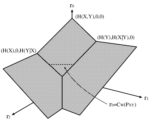
The region ${\cal R}_{\mathtt{GW}}^{*}(P_{XY})$ is contained in the outer region characterized by three planes (cf. Fig. 2):

$\displaystyle r_{0}+r_{1}+r_{2}$	$\displaystyle\geq H(X,Y),$	(188)
$\displaystyle r_{0}+r_{1}$	$\displaystyle\geq H(X),$	(189)
$\displaystyle r_{0}+r_{2}$	$\displaystyle\geq H(Y).$	(190)

The first plane is called the Pangloss plane in [6]. Let

	$\displaystyle{\cal H}(P_{XY})$	$\displaystyle:=\big\{(r_{0},r_{1},r_{2})\in{\cal R}_{\mathtt{GW}}(P_{XY}):r_{0}+r_{1}+r_{2}=H(X,Y)\big\}$		(191)
		$\displaystyle=\big\{(I(W\wedge X,Y),H(X\|W),H(Y\|W)):\|{\cal W}\|\leq\|{\cal X}\|\|{\cal Y}\|+2,~X-\!\!\circ\!\!-W-\!\!\circ\!\!-Y\big\}$		(192)

be the set of all achievable rate triplets on the Pangloss plane, where $X-\!\!\circ\!\!-W-\!\!\circ\!\!-Y$ means $(X,W,Y)$ form Markov chain. Although explicit characterization of ${\cal H}(P_{XY})$ is not clear in general, it is broader than the following triangular region

\displaystyle\mathtt{conv}\big\{(H(X,Y),0,0),~(H(Y),H(X|Y),0),~(H(X),0,H(Y|X))\big\},

(193)

and the altitude of the lowermost points is $r_{0}=C_{\mathtt{W}}(P_{XY})$ , where

	$\displaystyle C_{\mathtt{W}}(P_{XY})$	$\displaystyle:=\min\big\{r_{0}:\exists r_{1},r_{2}\mbox{ s.t. }(r_{0},r_{1},r_{2})\in{\cal H}(P_{XY})\big\}$		(194)
		$\displaystyle=\min\big\{I(W\wedge X,Y):\|{\cal W}\|\leq\|{\cal X}\|\|{\cal Y}\|,~X-\!\!\circ\!\!-W-\!\!\circ\!\!-Y\big\}$		(195)

is Wyner’s common information [38] (cf. Fig. 2).

When $(r_{0}^{*},r_{1}^{*},r_{2}^{*})\in{\cal H}(P_{XY})$ , it holds that

\displaystyle R(r_{1}^{*},r_{2}^{*}|P_{XY})=H(X,Y)-r_{1}^{*}-r_{2}^{*}.

(196)

Thus, $\lambda_{1}^{\star}=\lambda_{2}^{\star}=1$ . Also, since $(r_{0}^{*},r_{1}^{*},r_{2}^{*})$ is achieved by an optimal test channel satisfying $X-\!\!\circ\!\!-W^{\star}-\!\!\circ\!\!-Y$ , it holds that

	$\displaystyle\jmath_{XY}(x,y)$	$\displaystyle=\log\frac{P_{W\|XY}^{\star}(w\|x,y)}{P_{W^{\star}}(w)}+\lambda_{1}^{\star}\bigg(\log\frac{1}{P_{X\|W^{\star}}(x\|w)}-r_{1}^{}\bigg)+\lambda_{2}^{\star}\bigg(\log\frac{1}{P_{Y\|W^{\star}}(y\|w)}-r_{2}^{}\bigg)$		(197)
		$\displaystyle=\log\frac{1}{P_{XY}(x,y)}-r_{1}^{}-r_{2}^{}.$		(198)

Thus, the second-order region is characterized as follows:¹⁶¹⁶ 16 It is apparent from (196) that the second derivative of $R(r_{1},r_{2}|P_{\theta})$ around $(r_{1}^{*},r_{2}^{*},\theta(P_{XY}))$ is bounded. Furthermore, instead of checking differentiability of test channels, we can directly differentiate $\jmath_{XY}(x,y)$ in this case, and thus the validity of Lemma 3 is also guaranteed.

Corollary 2

When $(r_{0}^{*},r_{1}^{*},r_{2}^{*})$ is an strict inner point of ${\cal H}(P_{XY})$ ,¹⁷¹⁷ 17 Since we do not know an explicit form of ${\cal R}_{\mathtt{GW}}(P_{XY})$ outside ${\cal H}(P_{XY})$ , it is not clear if the regularity condition is satisfied or not on the boundary of ${\cal H}(P_{XY})$ . it holds that

\displaystyle{\cal L}_{\mathtt{GW}}(\varepsilon;r_{0}^{*},r_{1}^{*},r_{2}^{*})=\big\{(L_{0},L_{1},L_{2}):L_{0}+L_{1}+L_{2}\geq\sqrt{V_{XY}}\mathsf{Q}^{-1}(\varepsilon)\big\},

(199)

where $V_{XY}$ is given by

	$\displaystyle V_{XY}$	$\displaystyle=\mathsf{V}\big[\jmath_{XY}(X,Y)\big]$		(200)
		$\displaystyle=\mathsf{V}\bigg[\log\frac{1}{P_{XY}(X,Y)}\bigg].$		(201)

In fact, the sum constraint on the second-order rates in the above corollary coincides with the cooperative outer bound, where the two decoders cooperate. Thus, on the Pangloss plane, there is no sum-rate loss compared to cooperative decoding scheme up to the second-order, which is quite remarkable. However, it does not mean that the auxiliary random variable is not needed; the auxiliary random variable is needed to construct a code that achieve the optimal second-order region.

VI Discussion

In this paper, we derived a characterization of the second-order region of the Gray-Wyner network. Apart from the interest on this network itself, there is another motivation to study this problem. As we mentioned earlier, the characterization of the first-order region of multi-terminal problems typically involve auxiliary random variables; involvement of auxiliary random variables is one of reasons that the second-order analysis of multi-terminal problems is difficult. Thus, the result of this paper is an important step toward extending the second-order analysis to multi-terminal problems.

It seems that the next simple problems that involve auxiliary random variables are the coding problems with side-information (cf. [37]). In contrast to the Gray-Wyner network, the coding problems with side-information involve Markov chain structures on auxiliary random variables that stem from the distributed coding nature of the problems. Thus, the techniques used in this paper are not enough to solve these problems. However, we believe that the result in this paper at least gives some hints to tackle those problems.

Acknowledgement

The author would like to thank Yasutada Oohama and Vincent Y. F. Tan for valuable comments. The author also would like to thank Victoria Kostina for valuable comments; in particular, the reference [3, Remark in p. 69] in Footnote 8 was informed to the author from her.

References

[1] S. Amari and H. Nagaoka, Methods of Information Geometry. Oxford University Press, 2000.
[2] T. Berger, Rate Distortion Theory. Princeton-Hall Inc., 1971.
[3] I. Csiszár, “On an extremum problem of information theory,” Studia Scientiarum Mathematicarum Hungarica, vol. 9, pp. 57–71, 1974.
[4] I. Csiszár and J. Körner, Information Theory, Coding Theorems for Discrete Memoryless Systems, 2nd ed. Cambridge University Press, 2011.
[5] A. El Gamal and Y.-H. Kim, Network Information Theory. Cambridge, 2011.
[6] R. M. Gray and A. D. Wyner, “Source coding for a simple network,” Bell Labs. Technical Journal, vol. 53, no. 9, pp. 1681–1721, November 1974.
[7] W. Gu and M. Effros, “A strong converse for a collection of network source coding problems,” in Proc. IEEE Int. Symp. Inf. Theory 2009, 2009, pp. 2316–2320.
[8] ——, “A strong converse in source coding for super-source networks,” in Proc. IEEE Int. Symp. Inf. Theory 2011, 2011, pp. 395–399.
[9] M. Hayashi, “Second-order asymptotics in fixed-length source coding and intrinsic randomness,” IEEE Trans. Inform. Theory, vol. 54, no. 10, pp. 4619–4637, October 2008.
[10] ——, “Information spectrum approach to second-order coding rate in channel coding,” IEEE Trans. Inform. Theory, vol. 55, no. 11, pp. 4947–4966, November 2009.
[11] M. Hayashi, H. Tyagi, and S. Watanabe, “Secret key agreement: General capacity and second-order asymptotics,” 2014, arXiv:1411.0735.
[12] Y.-W. Huang and P. Moulin, “Finite blocklength coding for multiple access channels,” in Proc. IEEE Int. Symp. Inf. Theory 2012, Cambridge, MA, 2012, pp. 831–835.
[13] A. Ingber and Y. Kochman, “The dispersion of lossy source coding,” in Proc. Data Compression Conference, 2011, pp. 53–62.
[14] S. Kamath and V. Anantharam, “A new dual to the Gács-Körner common information defined via the Gray-Wyner system,” in Proc. Allerton Conference on Communication, Control and Computing, 2010, pp. 1340–1346.
[15] V. Kostina, “Lossy data compression: Nonasymptotic fundamental limits,” Ph.D. dissertation, Princeton University, Septermber 2013.
[16] V. Kostina and S. Verdú, “Fixed-length lossy compression in the finite blocklength regime,” IEEE Trans. Inform. Theory, vol. 58, no. 6, pp. 3309–3338, June 2012.
[17] ——, “Lossy joint source-channel coding in the finite blocklength regime,” IEEE Trans. Inform. Theory, vol. 59, no. 5, pp. 2545–2575, May 2013.
[18] ——, “Nonasymptotic noisy lossy source coding,” 2014, arXiv:1401.5125.
[19] ——, “Channels with cost constraints: Strong converse and dispersion,” IEEE Trans. Inform. Theory, vol. 61, no. 5, pp. 2415–2429, May 2015.
[20] S.-Q. Le, V. Y. F. Tan, and M. Motani, “A case where interference does not affect the channel dispersion,” IEEE Trans. Inform. Theory, vol. 61, no. 5, pp. 2439–2453, May 2015.
[21] E. MolavianJazi and J. N. Laneman, “Simpler achievable rate regions for multipleaccess with finite blocklength,” in Proc. IEEE Int. Symp. Inf. Theory 2012, Cambridge, MA, 2012, pp. 36–40.
[22] A. No, A. Ingber, and T. Weissman, “Strong successive refinability and rate-distortion-complexity tradeoff,” 2015, arXive:1506.03407.
[23] R. Nomura and T. S. Han, “Second-order resolvability, intrinsic randomness, and fixed-length source coding for mixed sources: Information spectrum approach,” IEEE Trans. Inform. Theory, vol. 59, no. 1, pp. 1–16, January 2013.
[24] ——, “Second-order Slepian-Wold coding theorems for non-mixed and mixed sources,” IEEE Trans. Inform. Theory, vol. 60, no. 9, pp. 5553–5572, September 2014.
[25] Y. Polyanskiy, H. V. Poor, and S. Verdu, “Channel coding rate in the finite blocklength regime,” IEEE Trans. Inform. Theory, vol. 56, no. 5, pp. 2307–2359, May 2010.
[26] J. Scarlett, “On the dispersions of the Gel’fand-Pinsker channel and dirty paper coding,” IEEE Trans. Inform. Theory, vol. 61, no. 9, pp. 4569–4586, September 2015.
[27] J. Scarlett, A. Martinez, and A. G. i Fábregas, “Second-order rate region of constant-composition codes for the multiple-access channel,” IEEE Trans. Inform. Theory, vol. 61, no. 1, pp. 157–172, January 2015.
[28] J. Scarlett and V. Y. F. Tan, “Second-order asymptotics for the Gaussian MAC with degraded message sets,” 2013, arXiv:1310.1197.
[29] V. Strassen, “Asymptotische Abschätzungen in Shannons Informationstheorie,” in Trans. Third. Prague Conf. Inf. Th., 1962, pp. 689–723.
[30] V. Y. F. Tan, Asymptotic Estimates in Information Theory with Non-Vanishing Error Probabilities. NOW Publishers: Foundation and Trends in Communication and Information Theory, 2014, vol. 11, no. 1-2.
[31] V. Y. F. Tan and O. Kosut, “On the dispersion of three network information theory problems,” IEEE Trans. Inform. Theory, vol. 60, no. 2, pp. 881–903, February 2014.
[32] M. Tomamichel and V. Y. F. Tan, “Second-order coding rates for channels with state,” IEEE Trans. Inform. Theory, vol. 60, no. 8, pp. 4427–4448, August 2014.
[33] H. Tyagi, S. Venkatakrishnan, P. Viswanath, and S. Watanabe, “Information complexity density and simulation of protocols,” 2015, arXiv:1504.05666.
[34] H. Tyagi, P. Viswanath, and S. Watanabe, “Interactive communication for data exchange,” in Proceedings of 2015 IEEE International Symposium on Information Theory, 2015, pp. 1806–1810.
[35] D. Wang, A. Ingber, and Y. Kochman, “The dispersion of joint source channel coding,” in Proc. Allerton Conference on Communication, Control and Computing, 2011, pp. 180–187.
[36] S. Watanabe and M. Hayashi, “Strong converse and second-order asymptotics of channel resolvability,” in Proc. IEEE Int. Symp. Inf. Theory 2014, Honolulu, Hawaii, 2014, pp. 1882–1886.
[37] S. Watanabe, S. Kuzuoka, and V. Y. F. Tan, “Non-asymptotic and second-order achievability bounds for coding with side-informationn,” IEEE Trans. Inform. Theory, vol. 61, no. 4, pp. 1574–1605, April 2015.
[38] A. D. Wyner, “The common information of two dependent random variables,” IEEE Trans. Inform. Theory, vol. 21, no. 2, pp. 163–179, March 1975.
[39] M. H. Yassaee, M. R. Aref, and A. Gohari, “A technique for deriving one-shot achievability results in network information theory,” 2013, arXiv:1303.0696.
[40] B. Yu and T. P. Speed, “A rate of convergence result for a universal $d$ -semifaithful code,” IEEE Trans. Inform. Theory, vol. 39, no. 3, pp. 813–820, May 1993.

$\displaystyle R(r_{1}^{},r_{2}^{}\|P_{XY})$	$\displaystyle=\min_{P_{\bar{W}}}\min_{P_{\hat{X}\|\hat{W}}}\min_{P_{\hat{Y}\|\hat{W}}}\min_{P_{W\|XY}}F(P_{W\|XY},P_{\bar{W}},P_{\hat{X}\|\hat{W}},P_{\hat{Y}\|\hat{W}})$	(39)
	$\displaystyle\leq\min_{P_{W\|XY}}F(P_{W\|XY},P_{W^{\star}},P_{X\|W^{\star}},P_{Y\|W^{\star}})$	(40)
	$\displaystyle\leq F(P_{W\|XY}^{\star},P_{W^{\star}},P_{X\|W^{\star}},P_{Y\|W^{\star}})$	(41)
	$\displaystyle=R(r_{1}^{},r_{2}^{}\|P_{XY}).$	(42)

	$\displaystyle P_{W\|XY}^{\star}(w\|x,y)$	$\displaystyle=P_{W^{\star}}(w)\exp\bigg\{\Lambda(x,y\|P_{W^{\star}},P_{X\|W^{\star}},P_{Y\|W^{\star}},\lambda_{1}^{\star},\lambda_{2}^{\star})$		(43)
		$\displaystyle~~~~~~~~~+\lambda_{1}^{\star}\bigg(r_{1}^{}-\log\frac{1}{P_{X\|W^{\star}}(x\|w)}\bigg)+\lambda_{2}^{\star}\bigg(r_{2}^{}-\log\frac{1}{P_{Y\|W^{\star}}(y\|w)}\bigg)\bigg\},$		(44)

	$\displaystyle\frac{\partial R(r_{1}^{},r_{2}^{}\|P_{\theta})}{\partial\theta_{i}}\bigg\|_{\theta=\xi}$	$\displaystyle=\sum_{x,y}\frac{\partial P_{\theta}(x,y)}{\partial\theta_{i}}\bigg\|_{\theta=\xi}\jmath_{X_{\xi}Y_{\xi}}(x,y)+\sum_{x,y}P_{\xi}(x,y)\frac{\partial\jmath_{X_{\theta}Y_{\theta}}(x,y)}{\partial\theta_{i}}\bigg\|_{\theta=\xi}$		(59)
		$\displaystyle=\jmath_{X_{\xi}Y_{\xi}}(i)-\jmath_{X_{\xi}Y_{\xi}}(m)+\sum_{x,y}P_{\xi}(x,y)\frac{\partial\jmath_{X_{\theta}Y_{\theta}}(x,y)}{\partial\theta_{i}}\bigg\|_{\theta=\xi}.$		(60)

	$\displaystyle nH(\bar{X}\|\bar{W})$	$\displaystyle\leq nr_{1}+2\|{\cal X}\|\|{\cal Y}\|\|{\cal W}\|\log n,$		(85)
	$\displaystyle nH(\bar{Y}\|\bar{W})$	$\displaystyle\leq nr_{2}+2\|{\cal X}\|\|{\cal Y}\|\|{\cal W}\|\log n,$		(86)

$\displaystyle\|H(\bar{X}\|\bar{W})-H(\bar{X}\|W)\|$	$\displaystyle\leq\|H(\bar{W},\bar{X})-H(W,\bar{X})\|+\|H(W)-H(\bar{W})\|$	(89)
	$\displaystyle\leq\frac{\|{\cal X}\|\|{\cal Y}\|\|{\cal W}\|}{n}\log\frac{\|{\cal X}\|\|{\cal W}\|}{\frac{\|{\cal X}\|\|{\cal Y}\|\|{\cal W}\|}{n}}+\frac{\|{\cal X}\|\|{\cal Y}\|\|{\cal W}\|}{n}\log\frac{\|{\cal W}\|}{\frac{\|{\cal X}\|\|{\cal Y}\|\|{\cal W}\|}{n}}$	(90)
	$\displaystyle\leq\frac{2\|{\cal X}\|\|{\cal Y}\|\|{\cal W}\|}{n}\log n,$	(91)