跳到论文正文
W Papers独立论文阅读器 arXiv:1508.04042 论文正文 计算阅读时间 · 0%
引用这篇论文根据当前论文元数据生成,正式投稿前建议核对。


License: arXiv.org perpetual non-exclusive license
arXiv:1508.04042v3 [cond-mat.stat-mech] 09 Nov 2015

Work fluctuation-dissipation trade-off in heat engines

Ken Funo Email: funo@cat.phys.s.u-tokyo.ac.jp Affiliation: Department of Physics, The University of Tokyo, 7-3-1 Hongo, Bunkyo-ku, Tokyo 113-0033, Japan    Masahito Ueda Affiliation: Department of Physics, The University of Tokyo, 7-3-1 Hongo, Bunkyo-ku, Tokyo 113-0033, Japan Affiliation: RIKEN Center for Emergent Matter Science (CEMS), Wako, Saitama 351-0198, Japan
August 24, 2026
Abstract

Reducing work fluctuation and dissipation in heat engines or, more generally, information heat engines that perform feedback control is vital to maximize their efficiency. The same problem arises when we attempt to maximize the efficiency of a given thermodynamic task that undergoes nonequilibrium processes for arbitrary initial and final states. We find that the most general trade-off relation between work fluctuation and dissipation applicable to arbitrary nonequilibrium processes is bounded from below by the information distance characterizing how far the system is from thermal equilibrium. The minimum amount of dissipation is found to be given in terms of the relative entropy and the Renyi divergence, both of which quantify the information distance between the state of the system and the canonical distribution. We give an explicit protocol that achieves the fundamental lower bound of the trade-off relation.

Recent developments in nonequilibrium statistical mechanics enable us to assign physical meanings to nonequilibrium entropies such as Shannon and von Neumann entropies in certain situations [3, 2, 1]. The information-theoretic analysis of thermodynamics starting from and ending at arbitrary nonequilibrium states has been carried out, as in encoding and erasure of information [5, 4, 3, 6]. An important subset of this category is the information heat engines [1, 7, 8, 12, 14, 15, 13, 9, 10, 11], since the measurement projects the state of the system into the postmeasurement state which is usually out of equilibrium. They play a pivotal role in controlling small thermodynamic systems that operate at the level of thermodynamic fluctuations. Viewing biological processes as information processing requires us to quantify thermodynamic costs of biological sensory adaptation in terms of information-theoretic quantities [16]. Suppressing both work fluctuation and dissipation as much as possible is vital to heat engines and thermodynamic tasks since reducing dissipation allows us to increase the efficiency and reducing work fluctuation makes it possible to supply an exact amount of work needed to complete a given task or to extract a definite amount of work from the system.

Considerable efforts have been devoted in search for a protocol that minimizes work fluctuation and dissipation under nonequilibrium situations. Previous studies have explored the regime around vanishing work fluctuation by using techniques known as single-shot statistical mechanics [17, 18, 19, 20, 21], and the regime around vanishing dissipation on the basis of the second law of thermodynamics [4, 3]. However, as we prove in the present work, these two aims (vanishing work fluctuation and vanishing dissipation) are incompatible. We find the trade-off relation between work fluctuation and dissipation with its fundamental lower bound set by the information distance characterizing the nonequilibriumness of the system. We also show that the bounds on dissipation in the single-shot (vanishing work fluctuation) and reversible (vanishing dissipation) regimes can be smoothly connected via the relative entropy [22] and the Renyi divergence [23], both of which quantify the information distance between the nonequilibrium distribution and the canonical distribution. We apply the trade-off relation to information heat engines, where the fundamental lower bound of the trade-off relation is characterized by the obtained information. Numerical simulations on an information heat engine based on a single-electron box [14, 15] are performed to verify the trade-off relation. We propose a method to construct explicit protocols that achieve the lower bound of the trade-off relation.

Main Results.— We define the extractable work from the system as a change of the internal energy that is not absorbed by the heat bath: W⁡[Γ]=Eλ0​(x)−Eλ1​(y)+Q⁡[Γ]W[\Gamma]=E_{\lambda_{0}}(x)-E_{\lambda_{1}}(y)+Q[\Gamma], where Γ\Gamma denotes the trajectory of the process, Q⁡[Γ]Q[\Gamma] is the heat absorbed by the system, and Eλ0​(x)E_{\lambda_{0}}(x) and Eλ1​(y)E_{\lambda_{1}}(y) are the initial and final energies of the eigenstates, respectively. For nonequilibrium initial and final states, the maximum extractable work from the system is quantified by the nonequilibrium free-energy difference [3, 1] −Δ​ℱ​(x,y)=ℱλ0​(x)−ℱλ1​(y)-\Delta\mathcal{F}(x,y)=\mathcal{F}_{\lambda_{0}}(x)-\mathcal{F}_{\lambda_{1}}(y), where ℱλ0​(x)=Eλ0​(x)−β−1​S​[pini​(x)]\mathcal{F}_{\lambda_{0}}(x)=E_{\lambda_{0}}(x)-\beta^{-1}S[p_{\mathrm{ini}}(x)], S⁡[q⁡(x)]=−ln⁡q⁡(x)S[q(x)]=-\ln q(x) is the Shannon entropy and β\beta is the inverse temperature of the heat bath. We define dissipation as the difference between the maximum extractable work and the actually extracted work:

σ⁡[Γ]=−β⁡(W⁡[Γ]+Δ​ℱ​(x,y)).\sigma[\Gamma]=-\beta(W[\Gamma]+\Delta\mathcal{F}(x,y)). (1)
Refer to caption
Figure 1: Trade-off relations. (a) Normalized standard deviation of dissipation σ\sigma versus that of work WW. The solid line shows the lower bound of the trade-off relation (2). (b) Average dissipation versus the standard deviation of work. The black solid curve shows the lower bound of the trade-off relation (3) and (4) for arbitrary initial and final states. If dαd_{\alpha} takes the minimum value D∞D_{\infty}, the lower bound is given by the dashed curve. For a thermalized final state, Δdα(pfin||pλ1can)=0\Delta d_{\alpha}(p_{\mathrm{fin}}||p^{\mathrm{can}}_{\lambda_{1}})=0 and the lower bound is given by the green solid curve. Each blue dot is obtained by a numerical simulation of a random quench of a five-level system followed by thermalization and isothermal expansion (see Supplementary material for details). (c) The abscissa shows the standard deviation of work normalized by that of the fluctuation of the obtained information, and the ordinate shows the dissipation normalized by the mutual information between the system and the measuring apparatus. The solid curve shows the lower bound of the trade-off relation (10) and (12). Blue dots are obtained by a numerical simulation of a Szilard engine in a single-electron box [15] as illustrated in the inset (see Supplementary material for details). Here nn denotes the excess number of electrons in the quantum dot, mm denotes the outcome of the measurement on nn, and ϵ\epsilon is the measurement error rate which is set to be ϵ=0.02\epsilon=0.02 in the numerical simulation. The relevant two states n=0n=0 and n=1n=1 are assumed to be degenerate and initially populated with equal probability. Depending on the outcome mm of the state measurement, the feedback control is performed by lowering the energy level of the mm state relative to the other. Finally, the two energy levels are relaxed to its initial (equal-energy) state through thermal contact with a heat bath.

The first main result of our work is the trade-off relation between work fluctuation and fluctuation in dissipation (see Supplementary material for the proof):

⟨W2⟩−⟨W⟩2+β−1​⟨σ2⟩−⟨σ⟩2\displaystyle\sqrt{\left\langle W^{2}\right\rangle-\left\langle W\right\rangle^{2}}+\beta^{-1}\sqrt{\left\langle\sigma^{2}\right\rangle-\left\langle\sigma\right\rangle^{2}}
≥⟨(Δ​ℱ)2⟩−⟨Δ​ℱ⟩2.\displaystyle\hskip 113.81102pt\geq\sqrt{\left\langle(\Delta\mathcal{F})^{2}\right\rangle-\left\langle\Delta\mathcal{F}\right\rangle^{2}}. (2)

This result implies that the sum of the work fluctuation and the fluctuation in dissipation is bounded from below by the fluctuation of the nonequilibrium free-energy difference Δ​ℱ\Delta\mathcal{F} (See Fig. 1 (a)). If the initial and final states are far from equilibrium, the lower bound of (2) becomes very large. The trade-off relation (2) indicates that work and dissipation cannot simultaneously take definite values; if we reduce work fluctuation, the fluctuation in entropy production inevitably increases, and vice versa.

Refer to caption
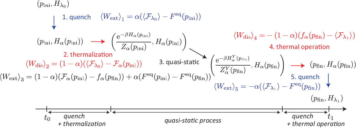
Figure 2: Protocol achieving the lower bounds of the trade-off relations. We denote (q,H)(q,H) as a pair of the state qq and the Hamiltonian HH. The transformation (pini,Hλ0)→(pfin,Hλ1)(p_{\mathrm{ini}},H_{\lambda_{0}})\rightarrow(p_{\mathrm{fin}},H_{\lambda_{1}}) that achieves minimum work fluctuation and dissipation is illustrated, where a change in the Hamiltonian is shown in a vertical direction and a change in the state is shown in a horizontal direction. The explicit protocol consists of five steps, where the extractable work ⟨Wext⟩\left\langle W_{\mathrm{ext}}\right\rangle and the dissipated work ⟨Wdis⟩:=β−1​⟨σ⟩\left\langle W_{\mathrm{dis}}\right\rangle:=\beta^{-1}\left\langle\sigma\right\rangle for each process are shown. Here, Hα​(pfin)H_{\alpha}(p_{\mathrm{fin}}) is a Hamiltonian which satisfies e−β​Hα​(pfin)/Zα(pfin):=(pfin)α(pλ1can)1−αe(1−α)Dα(pfin||pcanλ1)\mathrm{e}^{-\beta H_{\alpha}(p_{\mathrm{fin}})}/Z_{\alpha}(p_{\mathrm{fin}}):=(p_{\mathrm{fin}})^{\alpha}(p^{\mathrm{can}}_{\lambda_{1}})^{1-\alpha}\mathrm{e}^{(1-\alpha)D_{\alpha}(p_{\mathrm{fin}}||p^{\mathrm{can}}_{\lambda_{1}})}.

The second main result is the trade-off relation between work fluctuation and dissipation. From (2), there is a nontrivial relation between σ\sigma and WW if ⟨W2⟩−⟨W⟩2≤⟨(Δ​ℱ)2⟩−⟨Δ​ℱ⟩2\left\langle W^{2}\right\rangle-\left\langle W\right\rangle^{2}\leq\left\langle(\Delta\mathcal{F})^{2}\right\rangle-\left\langle\Delta\mathcal{F}\right\rangle^{2}. Then, let

α=⟨W2⟩−⟨W⟩2⟨(Δ​ℱ)2⟩−⟨Δ​ℱ⟩2,\alpha=\frac{\sqrt{\left\langle W^{2}\right\rangle-\left\langle W\right\rangle^{2}}}{\sqrt{\left\langle(\Delta\mathcal{F})^{2}\right\rangle-\left\langle\Delta\mathcal{F}\right\rangle^{2}}}, (3)

where α∈[0,1]\alpha\in[0,1]. In this case, dissipation and work satisfy the following inequalities (see Supplementary material for the proof):

⟨σ⟩\displaystyle\left\langle\sigma\right\rangle ≥\displaystyle\geq (1−α)(Δ𝒟α(pini||pλ0can)+Δdα(pfin||pλ1can)),\displaystyle(1-\alpha)(\Delta\mathcal{D}_{\alpha}(p_{\mathrm{ini}}||p_{\lambda_{0}}^{\mathrm{can}})+\Delta d_{\alpha}(p_{\mathrm{fin}}||p_{\lambda_{1}}^{\mathrm{can}})), (4)
⟨W⟩\displaystyle\left\langle W\right\rangle ≤\displaystyle\leq −α⁡⟨Δ​ℱ⟩−(1−α)​(fα​(pfin)−ℱα​(pini)).\displaystyle-\alpha\left\langle\Delta\mathcal{F}\right\rangle-(1-\alpha)\left(f_{\alpha}(p_{\mathrm{fin}})-\mathcal{F}_{\alpha}(p_{\mathrm{ini}})\right). (5)

Here, Δ​𝒟α=D−Dα\Delta\mathcal{D}_{\alpha}=D-D_{\alpha} (Δ​dα=dα−D\Delta d_{\alpha}=d_{\alpha}-D) gives the distance between the initial (final) distribution and the canonical distribution, D(pini||pλ0can)=∑xpini(x)lnpini​(x)pλ0can​(x)D(p_{\mathrm{ini}}||p_{\lambda_{0}}^{\mathrm{can}})=\sum_{x}p_{\mathrm{ini}}(x)\ln\frac{p_{\mathrm{ini}}(x)}{p_{\lambda_{0}}^{\mathrm{can}}(x)} is the Kullback-Leibler divergence (relative entropy) [22] and

Dα(pini||pλ0can)=1α−1ln[∑x(pini(x))α(pλ0can(x))1−α]D_{\alpha}(p_{\mathrm{ini}}||p^{\mathrm{can}}_{\lambda_{0}})=\frac{1}{\alpha-1}\ln\biggl[\sum_{x}(p_{\mathrm{ini}}(x))^{\alpha}(p_{\lambda_{0}}^{\mathrm{can}}(x))^{1-\alpha}\biggr] (6)

is the Renyi divergence [23]. Here dαd_{\alpha} is defined by

dα(pfin||pλ1can)=1α−1ln[∑y∈Y(pfin(y))α(pλ1can(y))1−α],d_{\alpha}(p_{\mathrm{fin}}||p_{\lambda_{1}}^{\mathrm{can}})=\frac{1}{\alpha-1}\ln\left[\sum_{y\in Y}(p_{\mathrm{fin}}(y))^{\alpha}(p_{\lambda_{1}}^{\mathrm{can}}(y))^{1-\alpha}\right], (7)

where the support YY is defined such that dαd_{\alpha} takes the smallest value that satisfies

dα(pfin||pλ1can)≥D∞(pfin||pλ1can)=lnmaxypfin​(y)pλ1can​(y).d_{\alpha}(p_{\mathrm{fin}}||p_{\lambda_{1}}^{\mathrm{can}})\geq D_{\infty}(p_{\mathrm{fin}}||p_{\lambda_{1}}^{\mathrm{can}})=\ln\max_{y}\frac{p_{\mathrm{fin}}(y)}{p_{\lambda_{1}}^{\mathrm{can}}(y)}. (8)

The lower bound of (4) is given by the black solid curve in Fig. 1 (b). The asymmetry between DαD_{\alpha} and dαd_{\alpha} is due to the absence of the time-reversed protocol of the thermalization process as discussed later. In (5), ⟨ℱλ0⟩=β−1D(pini||pλ0can)+Feq(pλ0can)\left\langle\mathcal{F}_{\lambda_{0}}\right\rangle=\beta^{-1}D(p_{\mathrm{ini}}||p_{\lambda_{0}}^{\mathrm{can}})+F^{\mathrm{eq}}(p^{\mathrm{can}}_{\lambda_{0}}) is the averaged nonequilibrium free-energy, and ℱα(pini)=β−1Dα(pini||pλ0can)+Feq(pλ0can)\mathcal{F}_{\alpha}(p_{\mathrm{ini}})=\beta^{-1}D_{\alpha}(p_{\mathrm{ini}}||p^{\mathrm{can}}_{\lambda_{0}})+F^{\mathrm{eq}}(p^{\mathrm{can}}_{\lambda_{0}}) is the α\alpha-generalization of the free energy, where we denote Feq​(q)F^{\mathrm{eq}}(q) as the equilibrium free energy whose corresponding canonical distribution is equal to the distribution qq. We also define the free energy fα(pfin)=β−1dα(pfin||pλ1can)+Feq(pλ1can)f_{\alpha}(p_{\mathrm{fin}})=\beta^{-1}d_{\alpha}(p_{\mathrm{fin}}||p_{\lambda_{1}}^{\mathrm{can}})+F^{\mathrm{eq}}(p^{\mathrm{can}}_{\lambda_{1}}) by using dαd_{\alpha}. We note that the ordering of the Renyi divergence [24] D∞≥D≥DαD_{\infty}\geq D\geq D_{\alpha} for 1≥α1\geq\alpha with (8) implies Δ​Dα≥0\Delta D_{\alpha}\geq 0 and Δ​dα≥0\Delta d_{\alpha}\geq 0.

Explicit protocol and the trade-off relation.— For given (pini,Hλ0)(p_{\mathrm{ini}},H_{\lambda_{0}}) and (pfin,Hλ1)(p_{\mathrm{fin}},H_{\lambda_{1}}), we want to find a protocol which connects them by reducing both work fluctuation and dissipation as much as possible. Although a quasi-static process makes both work fluctuation and dissipation vanish, we cannot directly connect (pini,Hλ0)→(pfin,Hλ1)(p_{\mathrm{ini}},H_{\lambda_{0}})\rightarrow(p_{\mathrm{fin}},H_{\lambda_{1}}) by the quasi-static process alone because the initial and final distributions are out of equilibrium. Instead, we prepare two canonical distributions as auxiliary intermediate states, and connect them by the quasi-static process. Then, we connect (pini,Hλ0)(p_{\mathrm{ini}},H_{\lambda_{0}}) with one of the canonical distributions by combining a quench process followed by thermalization, and the other canonical distribution is connected with (pfin,Hλ1)(p_{\mathrm{fin}},H_{\lambda_{1}}) by a thermal operation and a quench process. The entire protocol is illustrated in Fig. 3, and as we show in the Supplementary material, this protocol is necessary and sufficient to achieve the lower bound of (2) and (4).

Now let us discuss the explicit protocol in more detail and consider the physical meanings of the quantities that appear in (4) and (5). We change the initial distribution to the canonical distribution e−β​Hα​(pini)/Zα(pini):=(pini)α(pλ0can)1−αe(1−α)Dα(pini||pcanλ0)\mathrm{e}^{-\beta H_{\alpha}(p_{\mathrm{ini}})}/Z_{\alpha}(p_{\mathrm{ini}}):=(p_{\mathrm{ini}})^{\alpha}(p^{\mathrm{can}}_{\lambda_{0}})^{1-\alpha}\mathrm{e}^{(1-\alpha)D_{\alpha}(p_{\mathrm{ini}}||p^{\mathrm{can}}_{\lambda_{0}})}, which is an intermediate distribution between the initial state and the canonical distribution for the initial Hamiltonian. This is done by quenching the Hamiltonian from Hλ0H_{\lambda_{0}} to Hα​(pini)H_{\alpha}(p_{\mathrm{ini}}) and extract the work given by ⟨Wext⟩1=α⁡(⟨ℱλ0⟩−Feq​(pini))\left\langle W_{\mathrm{ext}}\right\rangle_{1}=\alpha(\left\langle\mathcal{F}_{\lambda_{0}}\right\rangle-F^{\mathrm{eq}}(p_{\mathrm{ini}})). Note that the maximum extractable from from the initial state is quantified by the nonequilibrium free energy ⟨ℱλ0⟩\left\langle\mathcal{F}_{\lambda_{0}}\right\rangle. The unexpended free energy (1−α)​⟨ℱλ0⟩(1-\alpha)\left\langle\mathcal{F}_{\lambda_{0}}\right\rangle is partly lost during the thermalization, and the remaining free energy, which can be extracted by the quasi-static process, is given by (1−α)​ℱα​(pini)(1-\alpha)\mathcal{F}_{\alpha}(p_{\mathrm{ini}}), as can be seen by noting the dissipated work due to the measurement: ⟨Wdis⟩2=(1−α)​(⟨ℱλ0⟩−ℱα​(pini))\left\langle W_{\mathrm{dis}}\right\rangle_{2}=(1-\alpha)(\left\langle\mathcal{F}_{\lambda_{0}}\right\rangle-\mathcal{F}_{\alpha}(p_{\mathrm{ini}})). This dissipation β⟨Wdis⟩2=(1−α)ΔDα(pini||pλ0can)=D(pini||e−β​Hα​(pini)/Zα(pini))\beta\left\langle W_{\mathrm{dis}}\right\rangle_{2}=(1-\alpha)\Delta D_{\alpha}(p_{\mathrm{ini}}||p^{\mathrm{can}}_{\lambda_{0}})=D(p_{\mathrm{ini}}||\mathrm{e}^{-\beta H_{\alpha}(p_{\mathrm{ini}})}/Z_{\alpha}(p_{\mathrm{ini}})) appears on the right-hand side of (4), which gives the information distance between the initial state and the canonical distribution which we connect during the thermalization process. Thus, the right-hand side of (5) is comprised of a part of the nonequilibrium free energy α​⟨ℱλ0⟩\alpha\left\langle\mathcal{F}_{\lambda_{0}}\right\rangle which can be extracted by the quench process and the free energy (1−α)​ℱα​(pini)(1-\alpha)\mathcal{F}_{\alpha}(p_{\mathrm{ini}}) which remains in the system after the thermalization.

The rest of the protocol is the transformation of the canonical distribution to the final state. Because we cannot perform time-reversal of the thermalization, we invoke a thermal operation [18] which transforms the state of the system by exchanging energy with the heat bath. This operation always changes the system closer to the thermal equilibrium, and we need to prepare a distribution whose “nonequilibriumness” is larger than that of the target final state. For this purpose, we prepare a localized distribution e−β​HαY​(pfin)/ZαY(pfin):=(pfin)α(pλ1can)1−αe(1−α)dα(pfin||pcanλ1)\mathrm{e}^{-\beta H_{\alpha}^{Y}(p_{\mathrm{fin}})}/Z^{Y}_{\alpha}(p_{\mathrm{fin}}):=(p_{\mathrm{fin}})^{\alpha}(p^{\mathrm{can}}_{\lambda_{1}})^{1-\alpha}\mathrm{e}^{(1-\alpha)d_{\alpha}(p_{\mathrm{fin}}||p^{\mathrm{can}}_{\lambda_{1}})}, whose support is restricted to YY. The term (1−α)​fα​(pfin)(1-\alpha)f_{\alpha}(p_{\mathrm{fin}}) is the free energy which is needed to prepare this localized thermal state and α​⟨ℱλ1⟩\alpha\left\langle\mathcal{F}_{\lambda_{1}}\right\rangle is the free energy needed to quench the Hamiltonian back to the final one (see (5) and Fig. 3). The asymmetry between the transformation of a nonequilibrium state into a thermalized state and its opposite transformation (i.e., from a thermalized state to a nonequilibrium state) gives rise to the difference between DαD_{\alpha} and dαd_{\alpha} (see (4)).

As shown in Ref. [18], the minimum work cost to create pfinp_{\mathrm{fin}} from a canonical distribution via the thermal operation with the fixed Hamiltonian Hα​(pfin)H_{\alpha}(p_{\mathrm{fin}}) is given by β−1D∞(pfin||e−β​Hα​(pfin)/Zα(pfin))\beta^{-1}D_{\infty}(p_{\mathrm{fin}}||\mathrm{e}^{-\beta H_{\alpha}(p_{\mathrm{fin}})}/Z_{\alpha}(p_{\mathrm{fin}})), with the help of a two-level auxiliary system. If we can introduce this auxiliary system, the dissipated work for the thermal operation is found to be ⟨Wdis⟩4=(1−α)​(ℱ∞​(pfin)−⟨ℱλ1⟩)\left\langle W_{\mathrm{dis}}\right\rangle_{4}=(1-\alpha)(\mathcal{F}_{\infty}(p_{\mathrm{fin}})-\left\langle\mathcal{F}_{\lambda_{1}}\right\rangle), and the equality condition in (8) is achieved (see Supplementary material for details). This condition is also achieved if the energy level of the system is dense. The lower bound of (4) with dα=D∞d_{\alpha}=D_{\infty} is shown by the dashed curve in Fig. 1 (b). Note that the solid curve jumps (i.e., the support YY changes) wherever the line touches the dashed curve because we take discrete energy levels.

Comparison with previous studies.— For α=1\alpha=1, (4) and (5) are equivalent to the second law of thermodynamics for arbitrary initial and final states: ⟨σ⟩≥0\left\langle\sigma\right\rangle\geq 0 and ⟨W⟩≤−⟨Δ​ℱ⟩\left\langle W\right\rangle\leq-\left\langle\Delta\mathcal{F}\right\rangle. Since the canonical distribution e−β​Hα​(pini)/Zα​(pini)\mathrm{e}^{-\beta H_{\alpha}(p_{\mathrm{ini}})}/Z_{\alpha}(p_{\mathrm{ini}}) is equal to the initial state for α=1\alpha=1 (the same relation holds for the final state), we do not need thermalization and the thermal operation to achieve the lower bound of the trade-off relations. Then, dissipation does not occur and we can extract the maximum average work from the system (see also Fig. 3). For α=0\alpha=0, (5) takes the form ⟨W⟩≤ℱ0​(pini)−f0​(pfin)\left\langle W\right\rangle\leq\mathcal{F}_{0}(p_{\mathrm{ini}})-f_{0}(p_{\mathrm{fin}}), which reproduce the single-shot results given in Refs. [17, 18]. Here, ℱ0​(pini)=−β−1​ln⁡[∑x∈Xexp⁡(−β​Eλ0​(x))]\mathcal{F}_{0}(p_{\mathrm{ini}})=-\beta^{-1}\ln[\sum_{x\in X}\exp(-\beta E_{\lambda_{0}}(x))] is equal to the equilibrium local free energy whose support XX is the same as the initial state. By raising the initially unoccupied energy levels, this amount of free energy remains after the thermalization.

For a general α\alpha, the trade-off relation gives the minimum amount of work fluctuation and dissipation in the intermediate regime. Comparing (3) and (5), we find that the distribution of the extractable work is broadened (meaning larger work fluctuation) if we want to increase the average value of work, and vice versa. Thus, the trade-off relation gives the best combinations of the “quality of work” and the average amount of extractable work. For equilibrium initial and final states, we can directly connect them by the quasi-static process and the lower bound of the trade-off relation (solid curve) in Fig. 1 (b) shrinks to a single point at the origin, i.e., work fluctuation and dissipation can both vanish.

Applications to information heat engines.— The information heat engines utilize the information obtained by the measurement to extract work from the system. For simplicity, we consider a classical system and assume that the premeasurement state pS​(x)p^{S}(x) is given by a canonical distribution. Then, dissipation is defined as the difference between the maximum amount of extractable work [13] −Δ​FS+β−1​IS​M-\Delta F^{S}+\beta^{-1}I^{SM} and the actually extracted work WS​[Γ]W^{S}[\Gamma]:

σ⁡[Γ]=−β⁡(WS​[Γ]+Δ​FS)+IS​M​(x,a),\sigma[\Gamma]=-\beta(W^{S}[\Gamma]+\Delta F^{S})+I^{SM}(x,a), (9)

and IS​M​(x,a)=ln⁡pS​M​(x,a)−ln⁡(pS​(x)​pM​(a))I^{SM}(x,a)=\ln p^{SM}(x,a)-\ln(p^{S}(x)p^{M}(a)) is the (unaveraged) classical mutual information between the system (SS) and the measurement apparatus (MM) [22]. Here, pS​M​(x,a)p^{SM}(x,a) is the joint probability distribution of S​MSM for the postmeasurement state, pS​(x)=∑apS​M​(x,a)p^{S}(x)=\sum_{a}p^{SM}(x,a) and pM​(a)=∑xpS​M​(x,a)p^{M}(a)=\sum_{x}p^{SM}(x,a). The trade-off relation (4) takes the following form (see also Fig. 1 (c)):

⟨σ⟩\displaystyle\left\langle\sigma\right\rangle ≥\displaystyle\geq (1−α)​(IS​M−IαS​M),\displaystyle(1-\alpha)(I^{SM}-I^{SM}_{\alpha}), (10)
β​⟨W⟩\displaystyle\beta\left\langle W\right\rangle ≤\displaystyle\leq α⁡⟨IS​M⟩+(1−α)​IαS​M−β​Δ​FS,\displaystyle\alpha\left\langle I^{SM}\right\rangle+(1-\alpha)I^{SM}_{\alpha}-\beta\Delta F^{S}, (11)

where α\alpha is defined by

α=β​⟨W2⟩−⟨W⟩2⟨(IS​M)2⟩−⟨IS​M⟩2,\alpha=\frac{\beta\sqrt{\left\langle W^{2}\right\rangle-\left\langle W\right\rangle^{2}}}{\sqrt{\left\langle(I^{SM})^{2}\right\rangle-\left\langle I^{SM}\right\rangle^{2}}}, (12)

and IαS​M=1α−1​ln​∑x,a(pS​M​(x,a))α​(pS​(x)​pM​(a))1−αI^{SM}_{\alpha}=\frac{1}{\alpha-1}\ln\sum_{x,a}(p^{SM}(x,a))^{\alpha}(p^{S}(x)p^{M}(a))^{1-\alpha} is the Renyi generalization of the mutual information. If we extract the maximum amount of work from the system for each measurement outcome, we can extract WS​[Γ]=−Δ​FS+β−1​I​(x,a)W^{S}[\Gamma]=-\Delta F^{S}+\beta^{-1}I(x,a) from the system, with finite work fluctuations. On the other hand, if we discard the measurement outcome, we can extract a definite amount of work WS​[Γ]=−Δ​FSW^{S}[\Gamma]=-\Delta F^{S} from the system with large dissipation. This means that (10) and (12) show a trade-off relation between work fluctuation and dissipation due to the fluctuation in the obtained information.

Possible experimental test of the trade-off relations.— The proposed trade-off relations can be tested by using the single electron box, which was used to realize a Szilard engine [14, 15]. Suppose that we prepare degenerate states of a two-level system and perform measurement to distinguish the state of the system which is initially distributed with equal probabilities P⁡(n=0)=P⁡(n=1)=1/2P(n=0)=P(n=1)=1/2, where nn labels the state of the system. Let the measurement error rate be ϵ\epsilon and the joint probability distribution of the system being nn and the measurement outcome being mm be given by P⁡(n,m)=(1−ϵ)/2P(n,m)=(1-\epsilon)/2 for m=nm=n and P⁡(n,m)=ϵ/2P(n,m)=\epsilon/2 for m≠nm\neq n. A feedback control is implemented by lowering the energy level of the state n=mn=m and let the energy-level return to the degeneracy point (see the inset of Fig. 1 (c)). By tracking the state of the system during this feedback, we can measure the extracted work for each run of the experiment, and calculate work fluctuation and dissipation. If we change the feedback protocol, e.g., by changing the degree of the energy-level shift, we obtain a different experimental data set of work fluctuation and dissipation. By plotting β​⟨W2⟩−⟨W⟩2/⟨(IS​M)2⟩−⟨IS​M⟩2\beta\sqrt{\left\langle W^{2}\right\rangle-\left\langle W\right\rangle^{2}}/\sqrt{\left\langle(I^{SM})^{2}\right\rangle-\left\langle I^{SM}\right\rangle^{2}} against ⟨σ⟩/⟨IS​M⟩\left\langle\sigma\right\rangle/\left\langle I^{SM}\right\rangle as shown in Fig. 1 (c), we can test the trade-off relation between work fluctuation and dissipation in information heat engines. The results of numerical simulations of a Szilard engine in a single-electron box using a master equation described in Ref. [15] are shown as dots in Fig. 1 (c).

Summary.— We have found a set of fundamental trade-off relations between work fluctuation and dissipation for nonequilibrium initial and final states. We can reproduce single-shot results in the limit of vanishing work fluctuation and thermodynamically reversible results (the lower bound of the conventional second law) in the limit of vanishing dissipation. These two limits are smoothly connected and the minimum dissipation along this boundary is characterized by the information distance between the state of the system and the canonical distribution. This result gives the fundamental bound on both work fluctuation and dissipation starting from and/or ending at nonequilibrium states. An application of the trade-off relation to information heat engines is discussed, including numerical simulations which vindicate the obtained trade-off relation.

Acknowledgements.
This work was supported by KAKENHI Grant No. 26287088 from the Japan Society for the Promotion of Science, a Grant-in-Aid for Scientific Research on Innovative Areas ‘Topological Materials Science’ (KAKENHI Grant No. 15H05855), the Photon Frontier Network Program from MEXT of Japan, and the Mitsubishi Foundation. K. F. acknowledges support from JSPS (Grant No. 254105) and through Advanced Leading Graduate Course for Photon Science (ALPS). K. F. thanks Hal Tasaki, Takahiro Sagawa, Jukka Pekola, Jonne Koski, Yûto Murashita, Tomohiro Shitara, Yusuke Horinouchi and Kohaku So for fruitful discussions and comments.

Appendix A Proof of the first main result

To show the first main result in Eq. (2) of the main text

⟨W2⟩−⟨W⟩2+β−1​⟨σ2⟩−⟨σ⟩2≥⟨(Δ​ℱ)2⟩−⟨Δ​ℱ⟩2,\sqrt{\left\langle W^{2}\right\rangle-\left\langle W\right\rangle^{2}}+\beta^{-1}\sqrt{\left\langle\sigma^{2}\right\rangle-\left\langle\sigma\right\rangle^{2}}\geq\sqrt{\left\langle(\Delta\mathcal{F})^{2}\right\rangle-\left\langle\Delta\mathcal{F}\right\rangle^{2}}, (13)

we first calculate the variance of σ+β​W\sigma+\beta W. By using Eq. (1) in the main text

σ⁡[Γ]=−β⁡(W⁡[Γ]+Δ​ℱ​(x,y)),\sigma[\Gamma]=-\beta(W[\Gamma]+\Delta\mathcal{F}(x,y)), (14)

we obtain

β2​(⟨W2⟩−⟨W⟩2)+⟨σ2⟩−⟨σ⟩2+2​β​(⟨σ​W⟩−⟨σ⟩​⟨W⟩)=⟨(Δ​ℱ)2⟩−⟨Δ​ℱ⟩2.\beta^{2}(\left\langle W^{2}\right\rangle-\left\langle W\right\rangle^{2})+\left\langle\sigma^{2}\right\rangle-\left\langle\sigma\right\rangle^{2}+2\beta(\left\langle\sigma W\right\rangle-\left\langle\sigma\right\rangle\left\langle W\right\rangle)=\left\langle(\Delta\mathcal{F})^{2}\right\rangle-\left\langle\Delta\mathcal{F}\right\rangle^{2}. (15)

Next, we consider the property of the variance-covariance matrix defined by

Vi​j=⟨(Xi−⟨Xi⟩)​(Xj−⟨Xj⟩)⟩.V_{ij}=\left\langle(X_{i}-\left\langle X_{i}\right\rangle)(X_{j}-\left\langle X_{j}\right\rangle)\right\rangle. (16)

The eigenvalues of Vi​jV_{ij} are positive semi-definite and thus the determinant of Vi​jV_{ij} is nonnegative. By taking X1=β​WX_{1}=\beta W and X2=σX_{2}=\sigma, and from Det​[Vi​j]≥0\text{Det}[V_{ij}]\geq 0, we obtain

(⟨W2⟩−⟨W⟩2)​(⟨σ2⟩−⟨σ⟩2)≥(⟨σ​W⟩−⟨σ⟩​⟨W⟩)2.(\left\langle W^{2}\right\rangle-\left\langle W\right\rangle^{2})(\left\langle\sigma^{2}\right\rangle-\left\langle\sigma\right\rangle^{2})\geq(\left\langle\sigma W\right\rangle-\left\langle\sigma\right\rangle\left\langle W\right\rangle)^{2}. (17)

Taking the square root of (17), we obtain

⟨W2⟩−⟨W⟩2​⟨σ2⟩−⟨σ⟩2≥⟨σ​W⟩−⟨σ⟩​⟨W⟩.\sqrt{\left\langle W^{2}\right\rangle-\left\langle W\right\rangle^{2}}\sqrt{\left\langle\sigma^{2}\right\rangle-\left\langle\sigma\right\rangle^{2}}\geq\left\langle\sigma W\right\rangle-\left\langle\sigma\right\rangle\left\langle W\right\rangle. (18)

Note that the above inequality holds trivially for ⟨σ​W⟩−⟨σ⟩​⟨W⟩≤0\left\langle\sigma W\right\rangle-\left\langle\sigma\right\rangle\left\langle W\right\rangle\leq 0. Combining (15) and (18), we obtain

(⟨W2⟩−⟨W⟩2+β−1​⟨σ2⟩−⟨σ⟩2)2≥⟨(Δ​ℱ)2⟩−⟨Δ​ℱ⟩2.\left(\sqrt{\left\langle W^{2}\right\rangle-\left\langle W\right\rangle^{2}}+\beta^{-1}\sqrt{\left\langle\sigma^{2}\right\rangle-\left\langle\sigma\right\rangle^{2}}\right)^{2}\geq\left\langle(\Delta\mathcal{F})^{2}\right\rangle-\left\langle\Delta\mathcal{F}\right\rangle^{2}. (19)

By taking the square root of either side of (19), we obtain the trade-off relation (13).

The equality condition in (13) is satisfied if and only if one of the eigenvalues of the matrix Vi​jV_{ij} is zero, i.e., if and only if there exist some constants aa and bb such that the variance of a​σ−b​β​Wa\sigma-b\beta W vanishes. Without the loss of generality, we can take a≥0a\geq 0.

Appendix B Proof of the second main result for an equilibrium final state

We first assume pfin​(y)=pλ1can​(y)p_{\mathrm{fin}}(y)=p_{\lambda_{1}}^{\mathrm{can}}(y) and prove the second main result. We discuss a more general case in Sec. D. From the assumption, Eq. (14) is given by

σ⁡[Γ]\displaystyle\sigma[\Gamma] =\displaystyle= −β​W​[Γ]−β​Feq​(pλ1can)+ℱλ0​(x)\displaystyle-\beta W[\Gamma]-\beta F^{\mathrm{eq}}(p^{\mathrm{can}}_{\lambda_{1}})+\mathcal{F}_{\lambda_{0}}(x) (20)
=\displaystyle= −β​W​[Γ]−β​Δ​Feq+ln⁡pini​(x)pλ0can​(x),\displaystyle-\beta W[\Gamma]-\beta\Delta F^{\mathrm{eq}}+\ln\frac{p_{\mathrm{ini}}(x)}{p_{\lambda_{0}}^{\mathrm{can}}(x)},

where Δ​Feq=Feq​(pλ1can)−Feq​(pλ0can)\Delta F^{\mathrm{eq}}=F^{\mathrm{eq}}(p^{\mathrm{can}}_{\lambda_{1}})-F^{\mathrm{eq}}(p^{\mathrm{can}}_{\lambda_{0}}) is the equilibrium free-energy difference, and the trade-off relation (13) takes the form

⟨W2⟩−⟨W⟩2+β−1​⟨σ2⟩−⟨σ⟩2≥⟨(ℱλ0)2⟩−⟨ℱλ02⟩.\sqrt{\left\langle W^{2}\right\rangle-\left\langle W\right\rangle^{2}}+\beta^{-1}\sqrt{\left\langle\sigma^{2}\right\rangle-\left\langle\sigma\right\rangle^{2}}\geq\sqrt{\left\langle(\mathcal{F}_{\lambda_{0}})^{2}\right\rangle-\left\langle\mathcal{F}_{\lambda_{0}}^{2}\right\rangle}. (21)

B.1 Detailed fluctuation theorem

We use the detailed fluctuation theorem which relates the ratio of the path probabilities and the total entropy production to prove the main results:

P⁡[Γ]P~​[Γ†]=eσ⁡[Γ],\frac{P[\Gamma]}{\tilde{P}[\Gamma^{\dagger}]}=e^{\sigma[\Gamma]}, (22)

where Γ\Gamma and Γ†\Gamma^{\dagger} denote the trajectories of the forward and backward (time-reversed) processes, and P⁡[Γ]P[\Gamma] and P~​[Γ†]\tilde{P}[\Gamma^{\dagger}] are the corresponding path probability distributions. Here,

σ⁡[Γ]=Δ​s​[Γ]−β​Q​[Γ]\sigma[\Gamma]=\Delta s[\Gamma]-\beta Q[\Gamma] (23)

is the total entropy production, where Δ​s​[Γ]=ln⁡pini​(x)−ln⁡pfin​(y)\Delta s[\Gamma]=\ln p_{\mathrm{ini}}(x)-\ln p_{\mathrm{fin}}(y) is a change in the Shannon entropy of the system. By using the definition of the nonequilibrium free energy, the total entropy production (23) is equal to Eq. (14). Note that Eq. (22) can be derived classically [26,27] and quantum-mechanically [27-30] for general settings (e.g., in the Hamiltonian dynamics and the stochastic dynamics). The following argument can also be applied to quantum systems if the initial density matrix of the system is diagonal in the initial energy eigenbasis.

B.2 Equality condition of the inequality (21)

Combining the detailed fluctuation theorem (22) and Eq. (20), we have

a​σ​[Γ]−b​β​W​[Γ]=b​β​Δ​Feq+(a+b)​ln⁡P⁡[Γ]P~​[Γ†]−b​ln⁡pini​(x)pλ0can​(x).a\sigma[\Gamma]-b\beta W[\Gamma]=b\beta\Delta F^{\mathrm{eq}}+(a+b)\ln\frac{P[\Gamma]}{\tilde{P}[\Gamma^{\dagger}]}-b\ln\frac{p_{\mathrm{ini}}(x)}{p_{\lambda_{0}}^{\mathrm{can}}(x)}. (24)

We set the condition

a​σ​[Γ]−b​β​W​[Γ]=b​β​Δ​Feq+ca\sigma[\Gamma]-b\beta W[\Gamma]=b\beta\Delta F^{\mathrm{eq}}+c (25)

to make the variance of a​σ−b​β​Wa\sigma-b\beta W vanish, where cc is a constant. Then, Eqs. (24) and (25) lead to

P⁡[Γ]P~​[Γ†]​(pini​(x)pλ0can​(x))−ba+b=exp⁡(ca+b).\frac{P[\Gamma]}{\tilde{P}[\Gamma^{\dagger}]}\left(\frac{p_{\mathrm{ini}}(x)}{p_{\lambda_{0}}^{\mathrm{can}}(x)}\right)^{\frac{-b}{a+b}}=\exp(\frac{c}{a+b}). (26)

The normalization of the backward probability distribution, i.e., ∑ΓP~​[Γ†]=1\sum_{\Gamma}\tilde{P}[\Gamma^{\dagger}]=1, combined with the relation P⁡[Γ]=P⁡[Γ|x]​pini​(x)P[\Gamma]=P[\Gamma|x]p_{\mathrm{ini}}(x), fixes the constant cc:

∑x(pλ0can​(x))ba+b​(pini​(x))aa+b=exp⁡(ca+b),\sum_{x}(p_{\lambda_{0}}^{\mathrm{can}}(x))^{\frac{b}{a+b}}(p_{\mathrm{ini}}(x))^{\frac{a}{a+b}}=\exp(\frac{c}{a+b}), (27)

where P⁡[Γ|x]P[\Gamma|x] is the conditional forward probability conditioned on xx and ∑Γ/xP⁡[Γ|x]=1\sum_{\Gamma/x}P[\Gamma|x]=1. By introducing the Renyi divergence, the constant cc takes the form

ca+b=−(1−α)Dα(pini||pλ0can),\frac{c}{a+b}=-(1-\alpha)D_{\alpha}(p_{\mathrm{ini}}||p_{\lambda_{0}}^{\mathrm{can}}), (28)

where α=a/(a+b)\alpha=a/(a+b). Using Eq. (27), σ\sigma and WW take the following forms:

σ⁡[Γ]\displaystyle\sigma[\Gamma] =\displaystyle= (1−α)(𝒟λ0(x)−Dα(pini||pλ0can)),\displaystyle(1-\alpha)\left(\mathcal{D}_{\lambda_{0}}(x)-D_{\alpha}(p_{\mathrm{ini}}||p_{\lambda_{0}}^{\mathrm{can}})\right), (29)
β​W​[Γ]\displaystyle\beta W[\Gamma] =\displaystyle= −βΔFeq+α𝒟λ0(x)+(1−α)Dα(pini||pλ0can),\displaystyle-\beta\Delta F^{\mathrm{eq}}+\alpha\mathcal{D}_{\lambda_{0}}(x)+(1-\alpha)D_{\alpha}(p_{\mathrm{ini}}||p_{\lambda_{0}}^{\mathrm{can}}), (30)

where 𝒟λ0​(x)=ln⁡pini​(x)−ln⁡pλ0can​(x)\mathcal{D}_{\lambda_{0}}(x)=\ln p_{\mathrm{ini}}(x)-\ln p_{\lambda_{0}}^{\mathrm{can}}(x). Note that ℱλ0​(x)=Feq​(pλ0can)+𝒟λ0​(x)\mathcal{F}_{\lambda_{0}}(x)=F^{\mathrm{eq}}(p^{\mathrm{can}}_{\lambda_{0}})+\mathcal{D}_{\lambda_{0}}(x). In particular, the first and the second terms on the left-hand side of (21) are given by

⟨σ2⟩−⟨σ⟩2\displaystyle\sqrt{\left\langle\sigma^{2}\right\rangle-\left\langle\sigma\right\rangle^{2}} =\displaystyle= β−1​|1−α|​⟨(ℱλ0)2⟩−⟨ℱλ0⟩2,\displaystyle\beta^{-1}|1-\alpha|\sqrt{\left\langle(\mathcal{F}_{\lambda_{0}})^{2}\right\rangle-\left\langle\mathcal{F}_{\lambda_{0}}\right\rangle^{2}}, (31)
⟨W2⟩−⟨W⟩2\displaystyle\sqrt{\left\langle W^{2}\right\rangle-\left\langle W\right\rangle^{2}} =\displaystyle= α​⟨(ℱλ0)2⟩−⟨ℱλ0⟩2.\displaystyle\alpha\sqrt{\left\langle(\mathcal{F}_{\lambda_{0}})^{2}\right\rangle-\left\langle\mathcal{F}_{\lambda_{0}}\right\rangle^{2}}. (32)

We conclude that the equality condition in (21) is satisfied if and only if Eqs. (29) and (30) hold and α\alpha takes the value in a range 0≤α≤10\leq\alpha\leq 1.

B.3 Proof of the second main result

Let us derive the second main result ((4) in the main text) for the case of pfin=pλ1canp_{\mathrm{fin}}=p_{\lambda_{1}}^{\mathrm{can}}:

⟨σ⟩≥(1−α)(D(pini||pλ0can)−𝒟α(pini||pλ0can)),\left\langle\sigma\right\rangle\geq(1-\alpha)(D(p_{\mathrm{ini}}||p_{\lambda_{0}}^{\mathrm{can}})-\mathcal{D}_{\alpha}(p_{\mathrm{ini}}||p_{\lambda_{0}}^{\mathrm{can}})), (33)

where the work fluctuation is assumed to be fixed (Eq. (3) in the main text) :

⟨W2⟩−⟨W⟩2=α​⟨(ℱλ0)2⟩−⟨ℱλ0⟩2\sqrt{\left\langle W^{2}\right\rangle-\left\langle W\right\rangle^{2}}=\alpha\sqrt{\left\langle(\mathcal{F}_{\lambda_{0}})^{2}\right\rangle-\left\langle\mathcal{F}_{\lambda_{0}}\right\rangle^{2}} (34)

where α∈[0,1]\alpha\in[0,1] is a parameter. We start by combining (21) and (34) and obtain

⟨σ2⟩−⟨σ⟩2≥(1−α)​⟨𝒟2⟩−⟨𝒟⟩2.\sqrt{\left\langle\sigma^{2}\right\rangle-\left\langle\sigma\right\rangle^{2}}\geq(1-\alpha)\sqrt{\left\langle\mathcal{D}^{2}\right\rangle-\left\langle\mathcal{D}\right\rangle^{2}}. (35)

Next, we expand the integral fluctuation theorem

⟨e−σ⟩=∑ΓP⁡[Γ]​P†​[Γ†]P⁡[Γ]=1\left\langle\mathrm{e}^{-\sigma}\right\rangle=\sum_{\Gamma}P[\Gamma]\frac{P^{\dagger}[\Gamma^{\dagger}]}{P[\Gamma]}=1 (36)

around σ⁡[Γ]=σα​[Γ]\sigma[\Gamma]=\sigma_{\alpha}[\Gamma] that achieves the lower bound of (35):

σα[Γ]=(1−α)(𝒟λ0(x)−Dα(pini||pλ0can)).\sigma_{\alpha}[\Gamma]=(1-\alpha)\left(\mathcal{D}_{\lambda_{0}}(x)-D_{\alpha}(p_{\mathrm{ini}}||p_{\lambda_{0}}^{\mathrm{can}})\right). (37)

From Eq. (36), we obtain

1\displaystyle 1 =\displaystyle= ⟨e−σ⟩=∑ΓP⁡[Γ]​e−(σ⁡[Γ]−σα​[Γ])−σα​[Γ]\displaystyle\left\langle\mathrm{e}^{-\sigma}\right\rangle=\sum_{\Gamma}P[\Gamma]\mathrm{e}^{-(\sigma[\Gamma]-\sigma_{\alpha}[\Gamma])-\sigma_{\alpha}[\Gamma]} (38)
=\displaystyle= ∑ΓPα​[Γ]​e−(σ⁡[Γ]−σα​[Γ]).\displaystyle\sum_{\Gamma}P_{\alpha}[\Gamma]\mathrm{e}^{-(\sigma[\Gamma]-\sigma_{\alpha}[\Gamma])}.

Here,

Pα[Γ]=P[Γ](pλ0can​(x)pini​(x))1−αe(1−α)Dα(pini||pλ0can)P_{\alpha}[\Gamma]=P[\Gamma]\left(\frac{p_{\lambda_{0}}^{\mathrm{can}}(x)}{p_{\mathrm{ini}}(x)}\right)^{1-\alpha}\mathrm{e}^{(1-\alpha)D_{\alpha}(p_{\mathrm{ini}}||p_{\lambda_{0}}^{\mathrm{can}})} (39)

gives the forward probability distribution in which the entropy production is close to σα​[Γ]\sigma_{\alpha}[\Gamma]. In fact, Pα​[Γ]=P~​[Γ†]P_{\alpha}[\Gamma]=\tilde{P}[\Gamma^{\dagger}] indicates that σ⁡[Γ]=σα​[Γ]\sigma[\Gamma]=\sigma_{\alpha}[\Gamma]. Expanding the exponent in Eq. (38) for small σ−σα\sigma-\sigma_{\alpha}, we have

0\displaystyle 0 =\displaystyle= ln⁡⟨e−(σ−σα)⟩α\displaystyle\ln\left\langle\mathrm{e}^{-(\sigma-\sigma_{\alpha})}\right\rangle_{\alpha} (40)
=\displaystyle= ln⁡⟨1−(σ−σα)+12​(σ−σα)2⟩α+O⁡((σ−σα)3).\displaystyle\ln\left\langle 1\right.-(\sigma-\sigma_{\alpha})+\frac{1}{2}(\sigma-\sigma_{\alpha})^{2}\left.\right\rangle_{\alpha}+O\left((\sigma-\sigma_{\alpha})^{3}\right).

We thus obtain the fluctuation-dissipation theorem near the point σα\sigma_{\alpha}:

2​⟨σ−σα⟩α=⟨(σ−σα)2⟩α−⟨σ−σα⟩α2+O⁡((σ−σα)3).2\left\langle\sigma-\sigma_{\alpha}\right\rangle_{\alpha}=\left\langle(\sigma-\sigma_{\alpha})^{2}\right\rangle_{\alpha}-\left\langle\sigma-\sigma_{\alpha}\right\rangle_{\alpha}^{2}+O\left((\sigma-\sigma_{\alpha})^{3}\right). (41)

Since the variance of σ\sigma is minimized if and only if σ⁡[Γ]=σα​[Γ]\sigma[\Gamma]=\sigma_{\alpha}[\Gamma], the average value of σ\sigma is also minimized for the same condition by using Eq. (41). Combining (35) and Eq. (41), we obtain the inequality (33).

Appendix C Explicit protocols that achieve the lower bound of the trade-off relations

Refer to caption
Figure 3: Protocols achieving the lower bounds of the trade-off relations for thermalized final states. The abscissa and ordinate show the state xx and energy of the system, respectively. The horizontal bars show the energy levels (the spectrum) of the Hamiltonian and the height of each rectangular box shows the probability distribution of the initial state pini​(x)p_{\mathrm{ini}}(x). We illustrate how the spectrum changes according to each protocol. After the change of the spectrum is completed, we attach a heat bath and quasi-statically change the Hamiltonian of the system to Hλ1H_{\lambda_{1}}. For α=1\alpha=1, we change the Hamiltonian to H⁡(pini)H(p_{\mathrm{ini}}), which is defined such that the canonical distribution with respect to H⁡(pini)H(p_{\mathrm{ini}}) is equal to the initial distribution. Dissipation does not occur while the system interacts with a heat bath. For α=0\alpha=0, we change the Hamiltonian by raising the energy levels to infinity, whose populations of the initial state are empty [17]. Note that work fluctuation vanishes during this process. For general α\alpha, we change the Hamiltonian to Hα​(pini)=(1−α)​Hλ0+α​H​(pini)H_{\alpha}(p_{\mathrm{ini}})=(1-\alpha)H_{\lambda_{0}}+\alpha H(p_{\mathrm{ini}}), i.e., we mix the changes of the energy levels of two protocols α=0\alpha=0 and α=1\alpha=1 by the ratio α:1−α\alpha:1-\alpha.

C.1 Reversible regime (α=1\alpha=1)

Let us first consider the case of α=1\alpha=1. The condition (26) is given by

P​[Γ]=P~​[Γ†],P[\Gamma]=\tilde{P}[\Gamma^{\dagger}], (42)

which means that the process is thermodynamically reversible, i.e., the backward protocol exactly brings the final state back into the initial state. The explicit protocol consists of two steps: (1) Change the Hamiltonian from Hλ0H_{\lambda_{0}} to H⁡(pini)H(p_{\mathrm{ini}}) while keeping the probability distribution pini​(x)p_{\mathrm{ini}}(x) fixed. The new Hamiltonian H⁡(pini)H(p_{\mathrm{ini}}) is chosen such that the canonical distribution with respect to H⁡(pini)H(p_{\mathrm{ini}}) is equal to pini​(x)p_{\mathrm{ini}}(x). (2) We change the Hamiltonian from H⁡(pini)H(p_{\mathrm{ini}}) to Hλ1H_{\lambda_{1}} slowly (quasi-static isothermal process). Since the time-reversal of these protocols (1) and (2) brings the final state pλ1can​(y)p_{\lambda_{1}}^{\mathrm{can}}(y) back to the initial state pini​(x)p_{\mathrm{ini}}(x), the condition (42) is satisfied. During the protocol (1), we change the energy levels of the system, which leads to a nonzero work fluctuation.

C.2 Single-shot regime (α=0\alpha=0)

Next, let us consider the case of α=0\alpha=0. The condition (26) is given by

P~​[Γ†]\displaystyle\tilde{P}[\Gamma^{\dagger}] =\displaystyle= P[Γ]pλ0can​(x)pini​(x)eD0(pini||pλ0can)\displaystyle P[\Gamma]\frac{p_{\lambda_{0}}^{\mathrm{can}}(x)}{p_{\mathrm{ini}}(x)}\mathrm{e}^{D_{0}(p_{\mathrm{ini}}||p_{\lambda_{0}}^{\mathrm{can}})} (43)
=\displaystyle= P⁡[Γ|x]​pλ0can,X​(x),\displaystyle P[\Gamma|x]p_{\lambda_{0}}^{\mathrm{can},X}(x),

where we introduce a conditional forward probability distribution P⁡[Γ|x]=P⁡[Γ]/pini​(x)P[\Gamma|x]=P[\Gamma]/p_{\mathrm{ini}}(x), and a local canonical distribution pλ0can,X(x)=exp(−βEλ0(x)+βFλ0+D0(pini||pλ0can))p_{\lambda_{0}}^{\mathrm{can},X}(x)=\exp(-\beta E_{\lambda_{0}}(x)+\beta F_{\lambda_{0}}+D_{0}(p_{\mathrm{ini}}||p_{\lambda_{0}}^{\mathrm{can}})) which has the same support X={x|pini​(x)≠0}X=\{x|p_{\mathrm{ini}}(x)\neq 0\} as the initial distribution. Now the condition (43) means that we should construct a process starting from pλ0can,X​(x)p_{\lambda_{0}}^{\mathrm{can},X}(x) which is thermodynamically reversible. Since the protocol λt\lambda_{t} starts from a Hamiltonian Hλ0H_{\lambda_{0}}, we need to consider the following two steps: (1) Change the Hamiltonian from Hλ0H_{\lambda_{0}} to a local Hamiltonian Hλ0X=∑x∈XEλ0​(x)H^{X}_{\lambda_{0}}=\sum_{x\in X}E_{\lambda_{0}}(x) by changing the energy levels labeled by x∉Xx\not\in X to infinity in the initial Hamiltonian H0H_{0}. Then, pλ0can,X​(x)p_{\lambda_{0}}^{\mathrm{can},X}(x) is equal to the canonical distribution with respect to Hλ0XH^{X}_{\lambda_{0}}. (2) Change the Hamiltonian from Hλ0XH^{X}_{\lambda_{0}} to Hλ1H_{\lambda_{1}} slowly in contact with the heat bath. Since the time reversal of these protocols (1) and (2) brings the final state pλ1can​(y)p_{\lambda_{1}}^{\mathrm{can}}(y) back to pλ0can,X​(x)p_{\lambda_{0}}^{\mathrm{can},X}(x), the condition in Eq. (43) is satisfied.

Now let us consider how the initial distribution changes by applying the protocols (1) and (2) described above. During the protocol (1), the probability distribution does not change. However, at the beginning of the protocol (2), the initial distribution thermalizes to pλ0can,X​(x)p_{\lambda_{0}}^{\mathrm{can},X}(x) because the change of the Hamiltonian from Hλ0XH^{X}_{\lambda_{0}} to Hλ1H_{\lambda_{1}} is slow. Finally, the distribution of the system is given by pλ1can​(y)p_{\lambda_{1}}^{\mathrm{can}}(y). Note that during the thermalization process, the work fluctuation is zero but the dissipation is nonzero.

C.3 Intermediate regime (general α\alpha)

Finally, we consider the case of general α\alpha. The condition (26) is given by

P~​[Γ†]\displaystyle\tilde{P}[\Gamma^{\dagger}] =\displaystyle= P[Γ](pλ0can​(x)pini​(x))(1−α)e(1−α)Dα(pini||pλ0can)\displaystyle P[\Gamma]\left(\frac{p_{\lambda_{0}}^{\mathrm{can}}(x)}{p_{\mathrm{ini}}(x)}\right)^{(1-\alpha)}\mathrm{e}^{(1-\alpha)D_{\alpha}(p_{\mathrm{ini}}||p_{\lambda_{0}}^{\mathrm{can}})} (44)
=\displaystyle= P⁡[Γ|x]​pα​(x),\displaystyle P[\Gamma|x]p_{\alpha}(x),

where

pα(x)=(pini(x))α(pλ0can(x))1−αe(1−α)Dα(pini||pλ0can)p_{\alpha}(x)=(p_{\mathrm{ini}}(x))^{\alpha}(p_{\lambda_{0}}^{\mathrm{can}}(x))^{1-\alpha}\mathrm{e}^{(1-\alpha)D_{\alpha}(p_{\mathrm{ini}}||p_{\lambda_{0}}^{\mathrm{can}})} (45)

is the canonical distribution with respect to the Hamiltonian Hα​(pini)=(1−α)​Hλ0+α​H​(pini)H_{\alpha}(p_{\mathrm{ini}})=(1-\alpha)H_{\lambda_{0}}+\alpha H(p_{\mathrm{ini}}). Following a similar argument for the protocol α=0\alpha=0, we can show that the explicit protocol is given by the following two steps: (1) Change the Hamiltonian of the system from Hλ0H_{\lambda_{0}} to Hα​(pini)H_{\alpha}(p_{\mathrm{ini}}) by keeping the initial distribution pini​(x)p_{\mathrm{ini}}(x) fixed; (2) Change the Hamiltonian from Hα​(pini)H_{\alpha}(p_{\mathrm{ini}}) to Hλ1H_{\lambda_{1}} slowly in contact with the heat bath. Due to this interaction with the heat bath, the distribution pinip_{\mathrm{ini}} thermalizes to the canonical distribution pαp_{\alpha} at the beginning of the protocol (2). Note that the explicit protocol is given by mixing two protocols α=0\alpha=0 and α=1\alpha=1 by the ratio α:1−α\alpha:1-\alpha. See Fig. 2 in the main text which describes a change in the energy levels in protocol (1).

Note that the protocol (1) described above can be thought of as an ordinary adiabatic process if we can turn off the interaction between the system and the heat bath during the control of the Hamiltonian. If the heat bath is always in contact with the system, we need to quench the Hamiltonian instantaneously.

Appendix D The case of a nonequilibrium final state

In this section, we consider the case in which the final state is out of equilibrium. Recall that the lower bound of (21) is satisfied if and only if the variance of α​σ−(1−α)​W\alpha\sigma-(1-\alpha)W is equal to zero, and the constant α\alpha takes a value between [0,1][0,1]. By setting the condition

a​σ​[Γ]−b​β​W​[Γ]=b​β​Δ​Feq+c′,a\sigma[\Gamma]-b\beta W[\Gamma]=b\beta\Delta F^{\mathrm{eq}}+c^{\prime}, (46)

we obtain a relation between forward and backward probability distributions:

exp⁡(c′)=P⁡[Γ]P~​[Γ†]​(pini​(x)pλ0can​(x))−(1−α)​(pfin​(y)pλ1can​(y))1−α,\exp(c^{\prime})=\frac{P[\Gamma]}{\tilde{P}[\Gamma^{\dagger}]}\left(\frac{p_{\mathrm{ini}}(x)}{p_{\lambda_{0}}^{\mathrm{can}}(x)}\right)^{-(1-\alpha)}\left(\frac{p_{\mathrm{fin}}(y)}{p_{\lambda_{1}}^{\mathrm{can}}(y)}\right)^{1-\alpha}, (47)

where c′c^{\prime} is a constant which will be determined later. We first identify an explicit condition on path probabilities which gives the lower bound of the trade-off relation (4) in the main text by rewriting the above condition (47):

P⁡[Γ|x]​pα​(x)=P~​[Γ†|y]​pα′​(y).P[\Gamma|x]p_{\alpha}(x)=\tilde{P}[\Gamma^{\dagger}|y]p_{\alpha}^{\prime}(y). (48)

Here, we use the definition of the canonical distribution pαp_{\alpha} with respect to the Hamiltonian HαH_{\alpha} given in Eq. (45). Similarly, we define the canonical distribution pα′p_{\alpha}^{\prime} with respect to Hα​(pfin)H_{\alpha}(p_{\mathrm{fin}}), where

pα′(y)=(pfin(y))α(pλ1can(y))1−αec′−(1−α)Dα(pini||pλ0can)p_{\alpha}^{\prime}(y)=(p_{\mathrm{fin}}(y))^{\alpha}(p_{\lambda_{1}}^{\mathrm{can}}(y))^{1-\alpha}\mathrm{e}^{c^{\prime}-(1-\alpha)D_{\alpha}(p_{\mathrm{ini}}||p_{\lambda_{0}}^{\mathrm{can}})} (49)

and Hα​(pfin)=(1−α)​Hλ1+α​H​(pfin)H_{\alpha}(p_{\mathrm{fin}})=(1-\alpha)H_{\lambda_{1}}+\alpha H(p_{\mathrm{fin}}). Here, the Hamiltonian H⁡(pfin)H(p_{\mathrm{fin}}) is defined such that the canonical distribution for H⁡(pfin)H(p_{\mathrm{fin}}) with the inverse temperature β\beta is equal to pfinp_{\mathrm{fin}}. Note that the constant c′c^{\prime} is determined by the normalization condition of the distribution (49).

The condition (48) is satisfied if the system Hamiltonian is slowly changed from HαH_{\alpha} to Hα​(pfin)H_{\alpha}(p_{\mathrm{fin}}). However, we should note that we cannot transform the distribution pα′p_{\alpha}^{\prime} to pfinp_{\mathrm{fin}} in contact with a heat bath, because we do not have a time-reversal protocol of the thermalization process. Due to this asymmetry in time, we consider a modified protocol in which the support of the distribution pα′​(y)p_{\alpha}^{\prime}(y) is restricted to y∈Yy\in Y. By invoking the idea of thermo-majorization (Ref. [18] in the main text) which is to be explained later, we determine YY in which pα′​(y)p_{\alpha}^{\prime}(y) can be transformed to pfin​(y)p_{\mathrm{fin}}(y) only by exchanging heat with the heat bath (i.e., vanishing work fluctuation). Then, the normalization condition fixes the constant c′c^{\prime}:

c′=(1−α)Dα(pini||pλ0can)+(1−α)dα(pfin||pλ1can)c^{\prime}=(1-\alpha)D_{\alpha}(p_{\mathrm{ini}}||p_{\lambda_{0}}^{\mathrm{can}})+(1-\alpha)d_{\alpha}(p_{\mathrm{fin}}||p_{\lambda_{1}}^{\mathrm{can}}) (50)

and

(1−α)dα(pfin||pλ1can)=−ln∑y∈Y(pfin(y))α(pλ1can(y))1−α.(1-\alpha)d_{\alpha}(p_{\mathrm{fin}}||p_{\lambda_{1}}^{\mathrm{can}})=-\ln\sum_{y\in Y}(p_{\mathrm{fin}}(y))^{\alpha}(p_{\lambda_{1}}^{\mathrm{can}}(y))^{1-\alpha}. (51)

Then,

pα′=e−β​HαY​(pfin)ZαY​(pfin):=(pfin)α(pλ1can)1−αe(1−α)dα(pfin||pλ1can),p_{\alpha}^{\prime}=\frac{\mathrm{e}^{-\beta H_{\alpha}^{Y}(p_{\mathrm{fin}})}}{Z_{\alpha}^{Y}(p_{\mathrm{fin}})}:=(p_{\mathrm{fin}})^{\alpha}(p_{\lambda_{1}}^{\mathrm{can}})^{1-\alpha}\mathrm{e}^{(1-\alpha)d_{\alpha}(p_{\mathrm{fin}}||p_{\lambda_{1}}^{\mathrm{can}})}, (52)

where HαY​(pfin)H_{\alpha}^{Y}(p_{\mathrm{fin}}) is obtained by taking the Hamiltonian Hα​(pfin)H_{\alpha}(p_{\mathrm{fin}}) and restricting its support to YY.

Now let us briefly review thermal operation and thermo-majorization which we use to determine YY. Let ρS\rho^{S} be a density matrix with no off-diagonal components in the energy eigenbasis of the system Hamiltonian HSH^{S}. Then, the thermal operation ℰ\mathcal{E} is defined by the following map

ℰ⁡(ρS)=TrB​[US​B​(ρS⊗σcanB)​U†S​B],\mathcal{E}(\rho^{S})=\text{Tr}_{B}[U^{SB}(\rho^{S}\otimes\sigma^{B}_{\mathrm{can}})U^{\dagger SB}], (53)

where σβB\sigma^{B}_{\beta} is the canonical distribution of the heat bath with respect to the Hamiltonian HBH^{B} with the inverse temperature β\beta, and TrB\text{Tr}_{B} denotes a partial trace over the degrees of freedom of the heat bath. We also require that the unitary operator US​BU^{SB} satisfies the energy conservation of the composite system:

[US​B,HS+HB]=0.[U^{SB},H^{S}+H^{B}]=0. (54)

Since the initial state does not have coherence, we can also think of ℰ\mathcal{E} as a stochastic map with total energy conservation for a classical system. From the total energy conservation, the internal energy change Δ​E\Delta E of the system is equal to the heat QQ transfered from the heat bath to the system, i.e., the work is zero during this operation.

Next, let {Eαpfin​(y)}\{E_{\alpha}^{p_{\mathrm{fin}}}(y)\} represent the eigenspectrum of the Hamiltonian Hα​(pfin)H_{\alpha}(p_{\mathrm{fin}}). We arrange the final state pfin​(y)p_{\mathrm{fin}}(y) according to the following order:

pfin​(y1)(Zα​(pfin))−1​e−β​Eαpfin​(y1)≥pfin​(y2)(Zα​(pfin))−1​e−β​Eαpfin​(y2)≥⋯.\frac{p_{\mathrm{fin}}(y_{1})}{(Z_{\alpha}(p_{\mathrm{fin}}))^{-1}\mathrm{e}^{-\beta E_{\alpha}^{p_{\mathrm{fin}}}(y_{1})}}\geq\frac{p_{\mathrm{fin}}(y_{2})}{(Z_{\alpha}(p_{\mathrm{fin}}))^{-1}\mathrm{e}^{-\beta E_{\alpha}^{p_{\mathrm{fin}}}(y_{2})}}\geq\cdots. (55)

Then, we plot a convex curve (Lorenz curve [31]) in the (y,x)(y,x) plane in which each point is given by

(pfin,e−β​Hα​(pfin)Zα​(pfin))=((pfin​(y1),e−β​Eαpfin​(y1)Zα​(pfin)),(∑i=12pfin​(yi),∑i=12e−β​Eαpfin​(yi)Zα​(pfin)),(∑i=13pfin​(yi),∑i=13e−β​Eαpfin​(yi)Zα​(pfin)),⋯,(1,1)),(p_{\mathrm{fin}},\frac{\mathrm{e}^{-\beta H_{\alpha}(p_{\mathrm{fin}})}}{Z_{\alpha}(p_{\mathrm{fin}})})=((p_{\mathrm{fin}}(y_{1}),\frac{\mathrm{e}^{-\beta E_{\alpha}^{p_{\mathrm{fin}}}(y_{1})}}{Z_{\alpha}(p_{\mathrm{fin}})}),(\sum_{i=1}^{2}p_{\mathrm{fin}}(y_{i}),\sum_{i=1}^{2}\frac{\mathrm{e}^{-\beta E_{\alpha}^{p_{\mathrm{fin}}}(y_{i})}}{Z_{\alpha}(p_{\mathrm{fin}})}),(\sum_{i=1}^{3}p_{\mathrm{fin}}(y_{i}),\sum_{i=1}^{3}\frac{\mathrm{e}^{-\beta E_{\alpha}^{p_{\mathrm{fin}}}(y_{i})}}{Z_{\alpha}(p_{\mathrm{fin}})}),\cdots,(1,1)), (56)

where Zα​(pfin)=∑ie−β​Eαpfin​(yi)Z_{\alpha}(p_{\mathrm{fin}})=\sum_{i}\mathrm{e}^{-\beta E_{\alpha}^{p_{\mathrm{fin}}}(y_{i})} is the partition function with respect to the Hamiltonian Hα​(pfin)H_{\alpha}(p_{\mathrm{fin}}). Note that the ordering (55) ensures that the curve (56) is convex. Then, it has been proven in Ref. [18] in the main text that a state transformation from pp to qq is possible by thermal operation (with the system Hamiltonian Hα​(pfin)H_{\alpha}(p_{\mathrm{fin}})) if and only if the curve (q,e−β​Hα​(pfin)Zα​(pfin))(q,\frac{\mathrm{e}^{-\beta H_{\alpha}(p_{\mathrm{fin}})}}{Z_{\alpha}(p_{\mathrm{fin}})}) is a subset of the curve (p,e−β​Hα​(pfin)Zα​(pfin))(p,\frac{\mathrm{e}^{-\beta H_{\alpha}(p_{\mathrm{fin}})}}{Z_{\alpha}(p_{\mathrm{fin}})}).

Refer to caption
Figure 4: (a) Lorenz curve and the definition of the support YY. We plot {∑i=1ke−β​Eαpfin​(yi)/Zα​(pfin)}k\{\sum_{i=1}^{k}\mathrm{e}^{-\beta E_{\alpha}^{p_{\mathrm{fin}}}(y_{i})}/Z_{\alpha}(p_{\mathrm{fin}})\}_{k} and {∑i=1kp⁡(yi)}k\{\sum_{i=1}^{k}p(y_{i})\}_{k} in the (x,y)(x,y) plane, where the curve p=e−β​HαY​(pfin)/ZαY​(pfin)p=\mathrm{e}^{-\beta H_{\alpha}^{Y}(p_{\mathrm{fin}})}/Z_{\alpha}^{Y}(p_{\mathrm{fin}}) is represented by the dashed line and p=pfinp=p_{\mathrm{fin}} is represented by the solid curve. The dotted line is an extension of the line connecting two points: (0,0)(0,0) and (e−β​Eαpfin​(y1)/Zα​(pfin),pfin​(y1))(\mathrm{e}^{-\beta E_{\alpha}^{p_{\mathrm{fin}}}(y_{1})}/Z_{\alpha}(p_{\mathrm{fin}}),p_{\mathrm{fin}}(y_{1})). The support YY is defined as the largest support such that the slope of the line e−β​HαY​(pfin)/ZαY​(pfin)\mathrm{e}^{-\beta H_{\alpha}^{Y}(p_{\mathrm{fin}})}/Z_{\alpha}^{Y}(p_{\mathrm{fin}}) is equal to or larger than that of the dotted line. Then, the thermo-majorization criterion tells us that the local equilibrium state e−β​HαY​(pfin)/ZαY​(pfin)\mathrm{e}^{-\beta H_{\alpha}^{Y}(p_{\mathrm{fin}})}/Z_{\alpha}^{Y}(p_{\mathrm{fin}}) can be transformed into pfinp_{\mathrm{fin}} via a thermal operation. (b) The case of introducing an auxiliary system. By introducing an auxiliary system, the joint probability distribution e−β​Hα​(pfin)/Zα​(pfin)⊗pϵA\mathrm{e}^{-\beta H_{\alpha}(p_{\mathrm{fin}})}/Z_{\alpha}(p_{\mathrm{fin}})\otimes p^{A}_{\mathrm{\epsilon}} can be transformed into pfin⊗pcanAp_{\mathrm{fin}}\otimes p^{A}_{\mathrm{can}} if the slope of the line e−β​Hα​(pfin)/Zα​(pfin)⊗pϵA\mathrm{e}^{-\beta H_{\alpha}(p_{\mathrm{fin}})}/Z_{\alpha}(p_{\mathrm{fin}})\otimes p^{A}_{\mathrm{\epsilon}} is equal to or larger than that of the line connecting two points: (0,0)(0,0) and (e−β⁡(Eαpfin​(y1)+ϵ)/(Zα​(pfin)​ZA),pfin​(y1)​e−β​ϵ/ZA)(\mathrm{e}^{-\beta(E_{\alpha}^{p_{\mathrm{fin}}}(y_{1})+\epsilon)}/(Z_{\alpha}(p_{\mathrm{fin}})Z^{A}),p_{\mathrm{fin}}(y_{1})\mathrm{e}^{-\beta\epsilon}/Z^{A}).

Now our task is to find a local canonical distribution e−β​HαY​(pfin)/ZαY​(pfin)\mathrm{e}^{-\beta H_{\alpha}^{Y}(p_{\mathrm{fin}})}/Z_{\alpha}^{Y}(p_{\mathrm{fin}}) with support YY such that by a thermal operation, it can be transformed to pfinp_{\mathrm{fin}}. By plotting two curves (pfin,e−β​Hα​(pfin)Zα​(pfin))(p_{\mathrm{fin}},\frac{\mathrm{e}^{-\beta H_{\alpha}(p_{\mathrm{fin}})}}{Z_{\alpha}(p_{\mathrm{fin}})}) and (e−β​HαY​(pfin)ZαY​(pfin),e−β​Hα​(pfin)Zα​(pfin))(\frac{\mathrm{e}^{-\beta H_{\alpha}^{Y}(p_{\mathrm{fin}})}}{Z_{\alpha}^{Y}(p_{\mathrm{fin}})},\frac{\mathrm{e}^{-\beta H_{\alpha}(p_{\mathrm{fin}})}}{Z_{\alpha}(p_{\mathrm{fin}})}) as in Fig. 4. (a), we conclude that the slope of the latter curve should be larger than that of the former:

1∑y∈Y(Zα​(pfin))−1​e−β​Eαpfin​(y)≥pfin​(y1)(Zα​(pfin))−1​e−β​Eαpfin​(y1).\frac{1}{\sum_{y\in Y}(Z_{\alpha}(p_{\mathrm{fin}}))^{-1}\mathrm{e}^{-\beta E_{\alpha}^{p_{\mathrm{fin}}}(y)}}\geq\frac{p_{\mathrm{fin}}(y_{1})}{(Z_{\alpha}(p_{\mathrm{fin}}))^{-1}\mathrm{e}^{-\beta E_{\alpha}^{p_{\mathrm{fin}}}(y_{1})}}. (57)

We choose the largest support of YY that satisfies the condition (57). We denote the eigenenergies Epfin​(y)E_{p_{\mathrm{fin}}}(y) and Eλ1​(y)E_{\lambda_{1}}(y) corresponding to the Hamiltonians H⁡(pfin)H(p_{\mathrm{fin}}) and Hλ1H_{\lambda_{1}}. We also introduce the partition functions Z⁡(pfin)=∑yexp⁡(−β​Epfin​(y))Z(p_{\mathrm{fin}})=\sum_{y}\exp(-\beta E_{p_{\mathrm{fin}}}(y)) and Zλ1=∑yexp⁡(−β​Eλ1​(y))Z_{\lambda_{1}}=\sum_{y}\exp(-\beta E_{\lambda_{1}}(y)). It follows from pfin​(y)=exp⁡(−β​Epfin​(y))/Z⁡(pfin)p_{\mathrm{fin}}(y)=\exp(-\beta E_{p_{\mathrm{fin}}}(y))/Z(p_{\mathrm{fin}}) that the Renyi divergence between the final and canonical distributions is given by

(α−1)Dα(pfin||pλ1can)=ln∑y(pfin(y))α(pλ1can(y))1−α=lnZα​(pfin)(Z⁡(pfin))α​(Zλ1)1−α.(\alpha-1)D_{\alpha}(p_{\mathrm{fin}}||p_{\lambda_{1}}^{\mathrm{can}})=\ln\sum_{y}(p_{\mathrm{fin}}(y))^{\alpha}(p_{\lambda_{1}}^{\mathrm{can}}(y))^{1-\alpha}=\ln\frac{Z_{\alpha}(p_{\mathrm{fin}})}{(Z(p_{\mathrm{fin}}))^{\alpha}(Z_{\lambda_{1}})^{1-\alpha}}. (58)

Using Eq. (58), the right-hand side of (57) can be expressed as

Zα​(pfin)​pfin​(y1)e−β​Eαpfin​(y1)\displaystyle\frac{Z_{\alpha}(p_{\mathrm{fin}})p_{\mathrm{fin}}(y_{1})}{\mathrm{e}^{-\beta E_{\alpha}^{p_{\mathrm{fin}}}(y_{1})}} =\displaystyle= Zα​(pfin)(Z⁡(pfin))α​(Zλ1)1−α​(pfin​(y1)pλ1can​(y1))1−α\displaystyle\frac{Z_{\alpha}(p_{\mathrm{fin}})}{(Z(p_{\mathrm{fin}}))^{\alpha}(Z_{\lambda_{1}})^{1-\alpha}}\left(\frac{p_{\mathrm{fin}}(y_{1})}{p_{\lambda_{1}}^{\mathrm{can}}(y_{1})}\right)^{1-\alpha} (59)
=\displaystyle= exp[(1−α)(D∞(pfin||pλ1can)−Dα(pfin||pλ1can))],\displaystyle\exp\left[(1-\alpha)(D_{\infty}(p_{\mathrm{fin}}||p_{\lambda_{1}}^{\mathrm{can}})-D_{\alpha}(p_{\mathrm{fin}}||p_{\lambda_{1}}^{\mathrm{can}}))\right],

where

D∞(p||q)=lnmaxyp⁡(y)q⁡(y)D_{\infty}(p||q)=\ln\max_{y}\frac{p(y)}{q(y)} (60)

is the Renyi divergence of order ∞\infty. The left-hand side of (57) can be expressed as

Zα​(pfin)∑y∈Ye−β​Eαpfin​(y)=exp[(1−α)(dα(pfin||pλ1can)−Dα(pfin||pλ1can))].\frac{Z_{\alpha}(p_{\mathrm{fin}})}{\sum_{y\in Y}\mathrm{e}^{-\beta E_{\alpha}^{p_{\mathrm{fin}}}(y)}}=\exp\left[(1-\alpha)(d_{\alpha}(p_{\mathrm{fin}}||p_{\lambda_{1}}^{\mathrm{can}})-D_{\alpha}(p_{\mathrm{fin}}||p_{\lambda_{1}}^{\mathrm{can}}))\right]. (61)

Now the condition (57) to determine YY is rewritten in terms of the Reny divergences as

exp[(1−α)(dα(pfin||pλ1can)−Dα(pfin||pλ1can))]≥exp[(1−α)(D∞(pfin||pλ1can)−Dα(pfin||pλ1can))].\exp\left[(1-\alpha)(d_{\alpha}(p_{\mathrm{fin}}||p_{\lambda_{1}}^{\mathrm{can}})-D_{\alpha}(p_{\mathrm{fin}}||p_{\lambda_{1}}^{\mathrm{can}}))\right]\geq\exp\left[(1-\alpha)(D_{\infty}(p_{\mathrm{fin}}||p_{\lambda_{1}}^{\mathrm{can}})-D_{\alpha}(p_{\mathrm{fin}}||p_{\lambda_{1}}^{\mathrm{can}}))\right]. (62)

We note that this condition can be expressed by using the Lorenz curve as shown in Fig. 4. (a). If the energy level Eαpfin​(y)E_{\alpha}^{p_{\mathrm{fin}}}(y) is dense, we can choose YY such that the equality condition of (62) holds. Also, if we can attach an auxiliary system, we can tune the energy level of the total system in such a manner that the equality condition of (62) holds as described in the next subsection.

Having established a method to determine YY, we can calculate the functional form of σ\sigma and WW for the boundary by combining Eqs. (47) and (50):

σ⁡[Γ]\displaystyle\sigma[\Gamma] =\displaystyle= (1−α)​(𝒟λ0​(x)−𝒟α−𝒟λ1​(y)+dα),\displaystyle(1-\alpha)(\mathcal{D}_{\lambda_{0}}(x)-\mathcal{D}_{\alpha}-\mathcal{D}_{\lambda_{1}}(y)+d_{\alpha}), (63)
β​W​[Γ]\displaystyle\beta W[\Gamma] =\displaystyle= −β​Δ​Feq+(1−α)​(𝒟α−dα)+α⁡(𝒟λ0​(x)−𝒟λ1​(y)),\displaystyle-\beta\Delta F^{\mathrm{eq}}+(1-\alpha)(\mathcal{D}_{\alpha}-d_{\alpha})+\alpha(\mathcal{D}_{\lambda_{0}}(x)-\mathcal{D}_{\lambda_{1}}(y)), (64)

where 𝒟λ1​(y)=ln⁡pfin​(y)−ln⁡pλ1can​(y)\mathcal{D}_{\lambda_{1}}(y)=\ln p_{\mathrm{fin}}(y)-\ln p_{\lambda_{1}}^{\mathrm{can}}(y) is the distance between the final state and the canonical distribution.

Let us now derive the trade-off relation between work fluctuation and dissipation for arbitrary initial and final states. We fix the amount of work fluctuation as

⟨W2⟩−⟨W⟩2=α​⟨(Δ​ℱ)2⟩−⟨Δ​ℱ⟩2,\sqrt{\left\langle W^{2}\right\rangle-\left\langle W\right\rangle^{2}}=\alpha\sqrt{\left\langle(\Delta\mathcal{F})^{2}\right\rangle-\left\langle\Delta\mathcal{F}\right\rangle^{2}}, (65)

where α∈[0,1]\alpha\in[0,1] is a constant. We use exactly the same method that we use in deriving (33) except that σα​[Γ]\sigma_{\alpha}[\Gamma] in the present case is given by Eq. (63). Then, for the fixed work fluctuation (65), the bounds on dissipation and the average work take the following forms:

⟨σ⟩\displaystyle\left\langle\sigma\right\rangle ≥\displaystyle\geq (1−α)(D(pini||pλ0can)−Dα(pini||pλ0can))+(1−α)(dα(pfin||pλ1can)−D(pfin||pλ1can)),\displaystyle(1-\alpha)(D(p_{\mathrm{ini}}||p_{\lambda_{0}}^{\mathrm{can}})-D_{\alpha}(p_{\mathrm{ini}}||p_{\lambda_{0}}^{\mathrm{can}}))+(1-\alpha)(d_{\alpha}(p_{\mathrm{fin}}||p_{\lambda_{1}}^{\mathrm{can}})-D(p_{\mathrm{fin}}||p_{\lambda_{1}}^{\mathrm{can}})), (66)
⟨W⟩\displaystyle\left\langle W\right\rangle ≤\displaystyle\leq −α⁡⟨Δ​ℱ⟩−(1−α)​(fα​(pfin)​(pfin)−Fα​(pfin)CLOSE.\displaystyle-\alpha\left\langle\Delta\mathcal{F}\right\rangle-(1-\alpha)(f_{\alpha}(p_{\mathrm{fin}})(p_{\mathrm{fin}})-F_{\alpha}(p_{\mathrm{fin}}). (67)

D.1 The case of introducing an auxiliary system

Here, we consider a different setup of a two-level auxiliary system AA, whose eigenenergies are given by EA​(0)=0,EA​(1)=ϵE^{A}(0)=0,\ E^{A}(1)=\epsilon. We construct a protocol which gives the equality condition of (62) in this setup. For simplicity, we first consider the case of α=0\alpha=0. We consider a transition from pλ1can⊗pϵAp^{\mathrm{can}}_{\lambda_{1}}\otimes p^{A}_{\epsilon} to pfin⊗pcanAp_{\mathrm{fin}}\otimes p^{A}_{\mathrm{can}} via a thermal operation, where pϵA​(0)=0,pϵA​(1)=1p^{A}_{\epsilon}(0)=0,p^{A}_{\epsilon}(1)=1. Note that the support of the joint distribution pλ1can⊗pϵAp^{\mathrm{can}}_{\lambda_{1}}\otimes p^{A}_{\epsilon} is restricted to (y,1){(y,1)}. Then,

d0(pfin⊗pcanA||pλ1can⊗pϵA)=lnpcanA(1)=β(ϵ−FA).d_{0}(p_{\mathrm{fin}}\otimes p^{A}_{\mathrm{can}}||p^{\mathrm{can}}_{\lambda_{1}}\otimes p^{A}_{\epsilon})=\ln p^{A}_{\mathrm{can}}(1)=\beta(\epsilon-F^{A}). (68)

If we choose ϵ\epsilon such that

D∞(pfin||pλ1can)=β(ϵ−FA)=d0(pfin⊗pcanA||pλ1can⊗pϵA),D_{\infty}(p_{\mathrm{fin}}||p_{\lambda_{1}}^{\mathrm{can}})=\beta(\epsilon-F^{A})=d_{0}(p_{\mathrm{fin}}\otimes p^{A}_{\mathrm{can}}||p^{\mathrm{can}}_{\lambda_{1}}\otimes p^{A}_{\epsilon}), (69)

the lower bound of the trade-off relation (66) in the case of α=0\alpha=0 is given by

⟨σ⟩≥D(pini||pλ0can)−D0(pini||pλ0can)+D∞(pfin||pλ1can)−D(pfin||pλ1can).\left\langle\sigma\right\rangle\geq D(p_{\mathrm{ini}}||p_{\lambda_{0}}^{\mathrm{can}})-D_{0}(p_{\mathrm{ini}}||p_{\lambda_{0}}^{\mathrm{can}})+D_{\infty}(p_{\mathrm{fin}}||p_{\lambda_{1}}^{\mathrm{can}})-D(p_{\mathrm{fin}}||p_{\lambda_{1}}^{\mathrm{can}}). (70)

Here, we note that the quantity ϵ−FA\epsilon-F^{A} is equal to the work cost of creating pϵAp^{A}_{\epsilon} starting from pcanAp^{A}_{\mathrm{can}}.

Next, let us consider the case of general α\alpha. In this case, we consider a transition from exp⁡(−β​Hα​(pfin))/Zα​(pfin)⊗pϵA\exp(-\beta H_{\alpha}(p_{\mathrm{fin}}))/Z_{\alpha}(p_{\mathrm{fin}})\otimes p^{A}_{\epsilon} to pfin⊗pcanAp_{\mathrm{fin}}\otimes p^{A}_{\mathrm{can}} via a thermal operation. This operation is possible if ϵ\epsilon satisfies

exp[(1−α)(D∞(pfin||pλ1can)−Dα(pfin||pλ1can))]=pfin​(y1)e−β​Eαpfin​(y1)/Zα​(pfin)=1e−β​ϵ/ZA,\exp\left[(1-\alpha)(D_{\infty}(p_{\mathrm{fin}}||p_{\lambda_{1}}^{\mathrm{can}})-D_{\alpha}(p_{\mathrm{fin}}||p_{\lambda_{1}}^{\mathrm{can}}))\right]=\frac{p_{\mathrm{fin}}(y_{1})}{\mathrm{e}^{-\beta E_{\alpha}^{p_{\mathrm{fin}}}(y_{1})}/Z_{\alpha}(p_{\mathrm{fin}})}=\frac{1}{\mathrm{e}^{-\beta\epsilon}/Z^{A}}, (71)

where ZA=1+e−β​ϵZ^{A}=1+\mathrm{e}^{-\beta\epsilon} is the partition function of AA (see Fig. 4. (b)). By noting that the initial and final probability distributions of the ancillary system are given by pϵAp^{A}_{\epsilon} and pcanAp^{A}_{\mathrm{can}}, Eq. (47) takes the form

exp⁡(c′)=P⁡[Γ]​pϵA​(z)P~​[Γ†]​pcanA​(z)​(pini​(x)pλ0can​(x))−(1−α)​(pfin​(y)pλ1can​(y))1−α.\exp(c^{\prime})=\frac{P[\Gamma]p^{A}_{\epsilon}(z)}{\tilde{P}[\Gamma^{\dagger}]p^{A}_{\mathrm{can}}(z)}\left(\frac{p_{\mathrm{ini}}(x)}{p_{\lambda_{0}}^{\mathrm{can}}(x)}\right)^{-(1-\alpha)}\left(\frac{p_{\mathrm{fin}}(y)}{p_{\lambda_{1}}^{\mathrm{can}}(y)}\right)^{1-\alpha}. (72)

Using the following expression

exp⁡(−β​Eαpfin​(y))Zα​(pfin)=(pfin(y))α(pλ1can(y))1−αe(1−α)Dα(pfin||pλ1can),\frac{\exp(-\beta E_{\alpha}^{p_{\mathrm{fin}}}(y))}{Z_{\alpha}(p_{\mathrm{fin}})}=(p_{\mathrm{fin}}(y))^{\alpha}(p_{\lambda_{1}}^{\mathrm{can}}(y))^{1-\alpha}\mathrm{e}^{(1-\alpha)D_{\alpha}(p_{\mathrm{fin}}||p_{\lambda_{1}}^{\mathrm{can}})}, (73)

the constant c′c^{\prime} is determined by

c′=(1−α)Dα(pini||pλ0can)+(1−α)Dα(pfin||pλ1can)−lnpcanA(1).c^{\prime}=(1-\alpha)D_{\alpha}(p_{\mathrm{ini}}||p_{\lambda_{0}}^{\mathrm{can}})+(1-\alpha)D_{\alpha}(p_{\mathrm{fin}}||p_{\lambda_{1}}^{\mathrm{can}})-\ln p^{A}_{\mathrm{can}}(1). (74)

Combining Eqs. (71) and (74), we obtain

c′=(1−α)Dα(pini||pλ0can)+(1−α)D∞(pfin||pλ1can).c^{\prime}=(1-\alpha)D_{\alpha}(p_{\mathrm{ini}}||p_{\lambda_{0}}^{\mathrm{can}})+(1-\alpha)D_{\infty}(p_{\mathrm{fin}}||p_{\lambda_{1}}^{\mathrm{can}}). (75)

If the energy level of the auxiliary system satisfies Eq. (71), the lower bound of the trade-off relation (66) is lowered and takes the form

⟨σ⟩≥(1−α)(D(pini||pλ0can)−Dα(pini||pλ0can))+(1−α)(D∞(pfin||pλ1can)−D(pfin||pλ1can)).\left\langle\sigma\right\rangle\geq(1-\alpha)(D(p_{\mathrm{ini}}||p_{\lambda_{0}}^{\mathrm{can}})-D_{\alpha}(p_{\mathrm{ini}}||p_{\lambda_{0}}^{\mathrm{can}}))+(1-\alpha)(D_{\infty}(p_{\mathrm{fin}}||p_{\lambda_{1}}^{\mathrm{can}})-D(p_{\mathrm{fin}}||p_{\lambda_{1}}^{\mathrm{can}})). (76)

D.2 Extractable work for each step of the protocol that achieve the lower bound of the trade-off relation

Here, we calculate the work and dissipation for each step of the explicit protocol. First, let us denote the canonical distributions as

e−β​Hα​(pini)Zα​(pini)\displaystyle\frac{\mathrm{e}^{-\beta H_{\alpha}(p_{\mathrm{ini}})}}{Z_{\alpha}(p_{\mathrm{ini}})} =\displaystyle= (pini)α​(pλ0can)1−α​e(1−α)​Dα,\displaystyle(p_{\mathrm{ini}})^{\alpha}(p^{\mathrm{can}}_{\lambda_{0}})^{1-\alpha}\mathrm{e}^{(1-\alpha)D_{\alpha}}, (77)
e−β​HαY​(pfin)ZαY​(pfin)\displaystyle\frac{\mathrm{e}^{-\beta H_{\alpha}^{Y}(p_{\mathrm{fin}})}}{Z_{\alpha}^{Y}(p_{\mathrm{fin}})} =\displaystyle= (pfin)α​(pλ1can)1−α​e(1−α)​dα,\displaystyle(p_{\mathrm{fin}})^{\alpha}(p^{\mathrm{can}}_{\lambda_{1}})^{1-\alpha}\mathrm{e}^{(1-\alpha)d_{\alpha}}, (78)

where

HαY​(pfin)=∑y∈YEαpfin​(y)H_{\alpha}^{Y}(p_{\mathrm{fin}})=\sum_{y\in Y}E_{\alpha}^{p_{\mathrm{fin}}}(y) (79)

is the local Hamiltonian whose support is restricted to YY and ZαY​(pfin)=∑y∈Yexp⁡(−β​Eαpfin​(y))Z_{\alpha}^{Y}(p_{\mathrm{fin}})=\sum_{y\in Y}\exp(-\beta E_{\alpha}^{p_{\mathrm{fin}}}(y)) is the corresponding partition function. Let us denote (p,H)(p,H) as the set of the distribution pp and the Hamiltonian HH. We also denote the nonequilibrium free energy as

ℱ(p,H)=Feq+β−1D(p||e−β​HZ),\mathcal{F}(p,H)=F^{\mathrm{eq}}+\beta^{-1}D(p||\frac{\mathrm{e}^{-\beta H}}{Z}), (80)

where FeqF^{\mathrm{eq}} is the equilibrium free energy with respect to the Hamiltonian HH. The explicit protocol that achieves the lower bound of (2), (4) and (5) is given by

  1. 1.

    Quench process (pini,Hλ0)→(pini,Hα​(pini))(p_{\mathrm{ini}},H_{\lambda_{0}})\rightarrow(p_{\mathrm{ini}},H_{\alpha}(p_{\mathrm{ini}})).

    The extractable work during this quench process is given by

    ⟨W⟩1\displaystyle\left\langle W\right\rangle_{1} =\displaystyle= ∑xpini​(x)​(Eλ0​(x)−Eαpini​(x))\displaystyle\sum_{x}p_{\mathrm{ini}}(x)(E_{\lambda_{0}}(x)-E_{\alpha}^{p_{\text{ini}}}(x)) (81)
    =\displaystyle= α​∑xpini​(x)​(Eλ0​(x)−Epini​(x))\displaystyle\alpha\sum_{x}p_{\mathrm{ini}}(x)(E_{\lambda_{0}}(x)-E_{p_{\mathrm{ini}}}(x))
    =\displaystyle= α⁡⟨ℱλ0⟩−α​Feq​(pini).\displaystyle\alpha\left\langle\mathcal{F}_{\lambda_{0}}\right\rangle-\alpha F^{\text{eq}}(p_{\mathrm{ini}}).
  2. 2.

    Thermalization process (pini,Hα​(pini))→(e−β​Hα​(pini)Zα​(pini),Hα​(pini))(p_{\mathrm{ini}},H_{\alpha}(p_{\mathrm{ini}}))\rightarrow(\frac{\mathrm{e}^{-\beta H_{\alpha}(p_{\mathrm{ini}})}}{Z_{\alpha}(p_{\mathrm{ini}})},H_{\alpha}(p_{\mathrm{ini}})).

    The extractable work vanishes and the dissipation is given by the nonequilibrium free-energy difference:

    β−1​⟨σ⟩2\displaystyle\beta^{-1}\left\langle\sigma\right\rangle_{2} =\displaystyle= ℱ⁡(pini,Hα​(pini))−ℱ⁡(e−β​Hα​(pini)/Zα​(pini),Hα​(pini))=(1−α)​(⟨ℱλ0⟩−ℱα)\displaystyle\mathcal{F}(p_{\mathrm{ini}},H_{\alpha}(p_{\mathrm{ini}}))-\mathcal{F}(\mathrm{e}^{-\beta H_{\alpha}(p_{\mathrm{ini}})}/Z_{\alpha}(p_{\mathrm{ini}}),H_{\alpha}(p_{\mathrm{ini}}))=(1-\alpha)(\left\langle\mathcal{F}_{\lambda_{0}}\right\rangle-\mathcal{F}_{\alpha}) (82)
    =\displaystyle= β−1D(pini||e−β​Hα​(pini)/Zα(pini))=(1−α)ΔDα(pini||pλ0can).\displaystyle\beta^{-1}D(p_{\mathrm{ini}}||\mathrm{e}^{-\beta H_{\alpha}(p_{\mathrm{ini}})}/Z_{\alpha}(p_{\mathrm{ini}}))=(1-\alpha)\Delta D_{\alpha}(p_{\mathrm{ini}}||p^{\mathrm{can}}_{\lambda_{0}}).
  3. 3.a.

    Quasi-static process (e−β​Hα​(pini)Zα​(pini),Hα​(pini))→(e−β​HαY​(pfin)ZαY​(pfin),HαY​(pfin))(\frac{\mathrm{e}^{-\beta H_{\alpha}(p_{\mathrm{ini}})}}{Z_{\alpha}(p_{\mathrm{ini}})},H_{\alpha}(p_{\mathrm{ini}}))\rightarrow(\frac{\mathrm{e}^{-\beta H_{\alpha}^{Y}(p_{\mathrm{fin}})}}{Z_{\alpha}^{Y}(p_{\mathrm{fin}})},H_{\alpha}^{Y}(p_{\mathrm{fin}})).

    The extractable work is equal to the equilibrium free-energy difference

    ⟨W⟩3\displaystyle\left\langle W\right\rangle_{3} =\displaystyle= Feq​(e−β​Hα​(pini)Zα​(pini))−Feq​(e−β​HαY​(pfin)ZαY​(pfin))\displaystyle F^{\mathrm{eq}}\left(\frac{\mathrm{e}^{-\beta H_{\alpha}(p_{\mathrm{ini}})}}{Z_{\alpha}(p_{\mathrm{ini}})}\right)-F^{\mathrm{eq}}\left(\frac{\mathrm{e}^{-\beta H_{\alpha}^{Y}(p_{\mathrm{fin}})}}{Z_{\alpha}^{Y}(p_{\mathrm{fin}})}\right) (83)
    =\displaystyle= (1−α)​ℱα​(pini)+α​Feq​(pini)−(1−α)​fα​(pfin)−α​Feq​(pfin).\displaystyle(1-\alpha)\mathcal{F}_{\alpha}(p_{\mathrm{ini}})+\alpha F^{\text{eq}}(p_{\mathrm{ini}})-(1-\alpha)f_{\alpha}(p_{\mathrm{fin}})-\alpha F^{\text{eq}}(p_{\mathrm{fin}}).
  4. 3.b.

    Quench process (e−β​HαY​(pfin)ZαY​(pfin),HαY​(pfin))→(e−β​HαY​(pfin)ZαY​(pfin),Hα​(pfin))(\frac{\mathrm{e}^{-\beta H_{\alpha}^{Y}(p_{\mathrm{fin}})}}{Z_{\alpha}^{Y}(p_{\mathrm{fin}})},H_{\alpha}^{Y}(p_{\mathrm{fin}}))\rightarrow(\frac{\mathrm{e}^{-\beta H_{\alpha}^{Y}(p_{\mathrm{fin}})}}{Z_{\alpha}^{Y}(p_{\mathrm{fin}})},H_{\alpha}(p_{\mathrm{fin}})).

    The extractable work and the dissipation both vanish during this process.

  5. 4.

    Thermal operation (e−β​HαY​(pfin)ZαY​(pfin),Hα​(pfin))→(pfin,Hα​(pfin))(\frac{\mathrm{e}^{-\beta H_{\alpha}^{Y}(p_{\mathrm{fin}})}}{Z_{\alpha}^{Y}(p_{\mathrm{fin}})},H_{\alpha}(p_{\mathrm{fin}}))\rightarrow(p_{\mathrm{fin}},H_{\alpha}(p_{\mathrm{fin}})).

    The extractable work vanishes and the dissipation is given by the nonequilibrium free-energy difference:

    β−1​⟨σ⟩4\displaystyle\beta^{-1}\left\langle\sigma\right\rangle_{4} =\displaystyle= ℱ⁡(e−β​HαY​(pfin)ZαY​(pfin),Hα​(pfin))−ℱ⁡(pfin,Hα​(pfin))\displaystyle\mathcal{F}\left(\frac{\mathrm{e}^{-\beta H_{\alpha}^{Y}(p_{\mathrm{fin}})}}{Z_{\alpha}^{Y}(p_{\mathrm{fin}})},H_{\alpha}(p_{\mathrm{fin}})\right)-\mathcal{F}(p_{\mathrm{fin}},H_{\alpha}(p_{\mathrm{fin}})) (84)
    =\displaystyle= (1−α)(fα(pfin)−⟨ℱλ1⟩)=(1−α)β−1Δdα(pfin||pλ1can).\displaystyle(1-\alpha)(f_{\alpha}(p_{\mathrm{fin}})-\left\langle\mathcal{F}_{\lambda_{1}}\right\rangle)=(1-\alpha)\beta^{-1}\Delta d_{\alpha}(p_{\mathrm{fin}}||p^{\mathrm{can}}_{\lambda_{1}}).
  6. 5.

    Quench process (pfin,Hα​(pfin))→(pfin,Hλ1)(p_{\mathrm{fin}},H_{\alpha}(p_{\mathrm{fin}}))\rightarrow(p_{\mathrm{fin}},H_{\lambda_{1}}).

    The extractable work is given by

    ⟨W⟩5=∑ypfin​(y)​(Eαpfin​(y)−Eλ1​(y))=−α⁡⟨ℱλ1⟩+α​Feq​(pfin).\left\langle W\right\rangle_{5}=\sum_{y}p_{\mathrm{fin}}(y)(E_{\alpha}^{p_{\mathrm{fin}}}(y)-E_{\lambda_{1}}(y))=-\alpha\left\langle\mathcal{F}_{\lambda_{1}}\right\rangle+\alpha F^{\mathrm{eq}}(p_{\mathrm{fin}}). (85)

By combining the extractable work and the dissipation given above, the lower bounds of (4) and (5) are obtained:

⟨σ⟩2+⟨σ⟩4\displaystyle\left\langle\sigma\right\rangle_{2}+\left\langle\sigma\right\rangle_{4} =\displaystyle= (1−α)ΔDα(pini||pλ0can)+(1−α)Δdα(pfin||pλ1can),\displaystyle(1-\alpha)\Delta D_{\alpha}(p_{\mathrm{ini}}||p^{\mathrm{can}}_{\lambda_{0}})+(1-\alpha)\Delta d_{\alpha}(p_{\mathrm{fin}}||p^{\mathrm{can}}_{\lambda_{1}}), (86)
⟨W⟩1+⟨W⟩3+⟨W⟩5\displaystyle\left\langle W\right\rangle_{1}+\left\langle W\right\rangle_{3}+\left\langle W\right\rangle_{5} =\displaystyle= α⁡(⟨ℱλ0⟩−⟨ℱλ1⟩)−(1−α)​(fα​(pfin)−ℱα​(pini)).\displaystyle\alpha(\left\langle\mathcal{F}_{\lambda_{0}}\right\rangle-\left\langle\mathcal{F}_{\lambda_{1}}\right\rangle)-(1-\alpha)(f_{\alpha}(p_{\mathrm{fin}})-\mathcal{F}_{\alpha}(p_{\mathrm{ini}})). (87)

By noting that fα​(q)≥ℱ∞​(q)≥ℱα​(q)f_{\alpha}(q)\geq\mathcal{F}_{\infty}(q)\geq\mathcal{F}_{\alpha}(q), extractable work starting from a nonequilibrium state is always smaller than the work cost of preparing a nonequilibrium final state starting from equilibrium, as shown in the case of α=0\alpha=0 in Ref. [18]. This relation holds for a general α\alpha with fixed work fluctuation except for the reversible regime α=1\alpha=1 because of the asymmetry of the protocol.

Appendix E Detailed description of the numerical simulations

E.1 Numerical simulation in Fig. 1. (b)

A numerical simulation is done in a five-level system, and we plotted the dissipation versus the work fluctuation in Fig. 1. (b) in the main text. We choose the initial distribution as pini​(x)={0.7,0.2,0.075,0.025,0}p_{\mathrm{ini}}(x)=\{0.7,0.2,0.075,0.025,0\}. We also set the canonical distribution with respect to the initial Hamiltonian Hλ0H_{\lambda_{0}} as pλ0can​(x)={0.5,0.3,0.1,0.075,0.025}p^{\mathrm{can}}_{\lambda_{0}}(x)=\{0.5,0.3,0.1,0.075,0.025\}. The numerical simulation is carried out by randomly generating a quenched Hamiltonian HquenchH_{\mathrm{quench}}. During this quenching process, work is put in or extracted from the system, given by W⁡(x)=Eλ0​(x)−Equench​(x)W(x)=E_{\lambda_{0}}(x)-E_{\mathrm{quench}}(x). Using this expression of work, we can calculate the work fluctuation along this process. After the quench of the Hamiltonian, we consider an ideal thermalization process in which the thermalized state is given by the canonical distribution pquenchcan​(x)p^{\mathrm{can}}_{\mathrm{quench}}(x) with respect to the quenched Hamiltonian HquenchH_{\mathrm{quench}}. The energy dissipated during this process is quantified by σ⁡(x)=ln⁡pini​(x)−ln⁡pquenchcan​(x)\sigma(x)=\ln p_{\mathrm{ini}}(x)-\ln p_{\mathrm{quench}}^{\mathrm{can}}(x). After the thermalization process, we consider an isothermal expansion by changing the Hamiltonian from HquenchH_{\mathrm{quench}} to Hλ1H_{\lambda_{1}}; then, the work fluctuation and the dissipation vanish during this process. Note that this idealized thermalization and isothermal processes are enough to explore the lower bound of the trade-off relation for the thermalized final state. We plot the following quantities for each quenched Hamiltonian in Fig. 1. (b):

⟨W2⟩−⟨W⟩2\displaystyle\left\langle W^{2}\right\rangle-\left\langle W\right\rangle^{2} =\displaystyle= ∑xpini​(x)​(W⁡(x))2−(∑xpini​(x)​W​(x))2,\displaystyle\sum_{x}p_{\mathrm{ini}}(x)(W(x))^{2}-\left(\sum_{x}p_{\mathrm{ini}}(x)W(x)\right)^{2}, (88)
⟨σ⟩\displaystyle\left\langle\sigma\right\rangle =\displaystyle= ∑xpini​(x)​σ​(x).\displaystyle\sum_{x}p_{\mathrm{ini}}(x)\sigma(x). (89)

In Fig. 1. (b), we choose pfin​(y)={0.6,0.2,0.1,0.075,0.025}p_{\mathrm{fin}}(y)=\{0.6,0.2,0.1,0.075,0.025\} and pλ1can​(y)={0.5,0.2,0.15,0.1,0.05}p^{\mathrm{can}}_{\lambda_{1}}(y)=\{0.5,0.2,0.15,0.1,0.05\} to calculate the lower bound of the trade-off relation for a target final state pfinp_{\mathrm{fin}}. Note that the support YY in the definition of dα(pfin||pλ1can)d_{\alpha}(p_{\mathrm{fin}}||p^{\mathrm{can}}_{\lambda_{1}}) changes from Y={0,1}Y=\{0,1\} to Y={0,1,2}Y=\{0,1,2\} around α=0.13\alpha=0.13 and from Y={0,1,2}Y=\{0,1,2\} to Y={0,1,2,3}Y=\{0,1,2,3\} around α=0.81\alpha=0.81.

E.2 Numerical simulation in Fig. 1 (c)

We consider a Szilard engine-like information heat engine in a single electron box in Fig. 1 (c) in the main text, following Ref. [15] in the main text (we also follow the parameters of numerical simulation described in the supplementary material of Ref. [15] in the main text). We consider a two-leveled system whose initial distribution is given by pS​(n)={12,12}p^{S}(n)=\{\frac{1}{2},\frac{1}{2}\}, where n={0,1}n=\{0,1\} labels the state of the system. The internal energy of the system is given by E⁡(n)=Ec​(n−ng)2E(n)=E_{\mathrm{c}}(n-n_{\mathrm{g}})^{2}, where EcE_{\mathrm{c}} is the total charging energy, ngn_{\mathrm{g}} is a control parameter which can tune the energy level of the system by changing the gate voltage. The initial and final Hamiltonians are given by setting ng=12n_{\mathrm{g}}=\frac{1}{2}.

We consider a measurement of the system, where the joint probability distribution of the state of the system being nn and the measurement outcome being mm is given by P⁡(n,m)=(1−ϵ)/2P(n,m)=(1-\epsilon)/2 for m=nm=n and P⁡(n,m)=ϵ/2P(n,m)=\epsilon/2 for m≠nm\neq n. Here, we set the error probability as ϵ=0.02\epsilon=0.02. For example, the postmeasurement state conditioned on the measurement outcome m=0m=0 is given by P⁡(n|m=0)={1−ϵ,ϵ}P(n|m=0)=\{1-\epsilon,\epsilon\}. We change the control parameter ngn_{\mathrm{g}} depending on the measurement outcome. One typical example (for m=0m=0) is to change ngn_{\mathrm{g}} to nquench=0.349n_{\text{quench}}=0.349 instantaneously, followed by a slow return to the degeneracy point:

ng​(t)=nquench+(0.5−nquench)​log⁡(1+t)log⁡(1+T),n_{\mathrm{g}}(t)=n_{\text{quench}}+(0.5-n_{\text{quench}})\frac{\log(1+t)}{\log(1+T)}, (90)

where tt is the time and TT is the total time needed to complete the feedback control. Note that nquenchn_{\text{quench}} is determined from the condition that the canonical distribution with respect to the Hamiltonian with ng=nquenchn_{\mathrm{g}}=n_{\text{quench}} is equal to the distribution of the postmeasurement state.

The probability distribution during the feedback control is numerically calculated by using the following master equation

d​P​(n=0,t)d​t\displaystyle\frac{\mathrm{d}P(n=0,t)}{\mathrm{d}t} =\displaystyle= −Γ0→1​(t)​P​(n=0,t)+Γ1→0​(t)​P​(n=1,t),\displaystyle-\Gamma_{0\rightarrow 1}(t)P(n=0,t)+\Gamma_{1\rightarrow 0}(t)P(n=1,t),
d​P​(n=1,t)d​t\displaystyle\frac{\mathrm{d}P(n=1,t)}{\mathrm{d}t} =\displaystyle= −Γ1→0​(t)​P​(n=1,t)+Γ0→1​(t)​P​(n=0,t),\displaystyle-\Gamma_{1\rightarrow 0}(t)P(n=1,t)+\Gamma_{0\rightarrow 1}(t)P(n=0,t), (91)

where P⁡(n,t)P(n,t) is the probability distribution of the system being nn at time tt, and Γ0→1​(t)\Gamma_{0\rightarrow 1}(t) is the tunneling rate of the single-electron box at time tt for the transition 0→10\rightarrow 1 using the expression given in Ref. [15] in the main text. The work is determined by the energy change of the system by changing the external parameter ng​(t)n_{\mathrm{g}}(t):

W⁡(n,t)=Et​(n)−Et+Δ​t​(n),W(n,t)=E_{t}(n)-E_{t+\Delta t}(n), (92)

where Et​(n)=Ec​(n−ng​(t))2E_{t}(n)=E_{\mathrm{c}}(n-n_{\mathrm{g}}(t))^{2} is the energy of the system at time tt. The average extractable work from the system and work fluctuation are given by

⟨W⟩\displaystyle\left\langle W\right\rangle =\displaystyle= ∑i,nW⁡(n,i​Δ​t)​P​(n,i​Δ​t),\displaystyle\sum_{i,n}W(n,i\Delta t)P(n,i\Delta t), (93)
⟨W2⟩−⟨W⟩2\displaystyle\left\langle W^{2}\right\rangle-\left\langle W\right\rangle^{2} =\displaystyle= ∑i{∑nW​(n,i​Δ​t)2​P​(n,i​Δ​t)−(∑nW⁡(n,i​Δ​t)​P​(n,i​Δ​t))2},\displaystyle\sum_{i}\left\{\sum_{n}W(n,i\Delta t)^{2}P(n,i\Delta t)-\left(\sum_{n}W(n,i\Delta t)P(n,i\Delta t)\right)^{2}\right\}, (94)

where Δ​t\Delta t is the discretized time step. Different types of feedback protocols are obtained by changing nquenchn_{\mathrm{quench}}, TT and the functional form of ng​(t)n_{\mathrm{g}}(t). For each feedback protocol, we calculate the dissipation and the work fluctuation, and plot them in Fig. 1 (c).

References

  • [1] Parrondo, J. M. R., Horowitz, J. M. & Sagawa, Nat. Phys. 11, 131 (2015).
  • [2] Deffner, S. & Lutz, E. Preprint at http://arXiv.org/abs/1201.3888 (2012).
  • [3] Esposito, M. & Van den Broeck, C. Euro. Phys. Lett. 95, 40004 (2011).
  • [4] Hasegawa, H.-H., Ishikawa, J., Takara, K. & Driebe, D. J. Phys. Lett. A 374, 1001 (2010).
  • [5] Landauer, R. IBM J. Res. Dev. 5, 183-191 (1961).
  • [6] Bérut, A., Arakelyan, A., Petrosyan, A., Ciliberto, S., Dillenschneider, R. & Lutz, E. Nature 483, 187-189 (2012).
  • [7] Maxwell, J. C. Theory of Heat (Appleton, London, 1871).
  • [8] Leff, H. S. & Rex, A. F. Maxwell’s Demon 2: Entropy, Classical and Quantum Information, Computing (Institute of Physics Publishing, 2003).
  • [9] Maruyama, K., Nori, F. & Vedral, V. Rev. Mod. Phys. 81, 1-23 (2009).
  • [10] Sagawa & T., Ueda, M. Phys. Rev. Lett. 100, 080403 (2008).
  • [11] Sagawa & T., Ueda, M. Phys. Rev. Lett. 102, 250602 (2009).
  • [12] Toyabe, S., Sagawa, T., Ueda, M., Muneyuki, E. & Sano, M. Nat. Phys. 6, 988 (2010).
  • [13] Sagawa & T., Ueda, M. Phys. Rev. Lett. 109, 180602 (2012).
  • [14] Koski, J. V., Maisi, V. F., Sagawa, T. & Pekola, J. P. Phys. Rev. Lett. 113, 030601 (2014).
  • [15] Koski, J. V., Maisi, V. F., Pekola, J. P. & Averin, D. V. PNAS 111, 13786 (2014).
  • [16] Sartori, P., Granger, L., Lee, C. F. & Horowitz, J. M. PLoS Comput. Biol. 10(12): e1003974 (2014).
  • [17] Å\ring{\mathrm{A}}berg, J. Nat. Commun. 4, 1925 (2013).
  • [18] Horodecki, M. & Oppenheim, J. Nat. Commun. 4, 2059 (2013).
  • [19] Branda~\tilde{\mathrm{a}}o, F. G. S. L., Horodecki, M., Oppenheim, J., Renes, J. M. & Spekkens, R. W. Phys. Rev. Lett. 111, 250404 (2013).
  • [20] Branda~\tilde{\mathrm{a}}o, F. G. S. L., Horodecki, M., Ng, N. H. Y., Oppenheim, J. & Wehner, S. PNAS 112, 3275 (2015).
  • [21] Lostaglio, M., Jennings, D. & Rudolph, T. Nat. Commun. 6, 6383 (2015).
  • [22] Nielsen, M. A. & Chuang, I. L. Quantum Computation and Quantum Information (Cambridge University Press, Cambridge, England, 2000).
  • [23] Rényi, A., Rev. Int. Stat. Inst. 33, 1 (1965).
  • [24] van Erven, T. & Harremoës, P. IEEE Int. Symp. Inf. Theory, vol.60, no.7, 3797-3820 (2014).
  • [25] Crooks, G. E. Phys. Rev. E 60, 2721-2726 (1999).
  • [26] Seifert, U. Rep. Prog. Phys. 75, 126001 (2012).
  • [27] Crooks, G. E. J. Stat. Mech.: Theor. Exp. P10023 (2008).
  • [28] Campisi, M., Hänggi, P. & Talkner, P. Rev. Mod. Phys. 83 771 (2011).
  • [29] Horowitz, J. M. Phys. Rev. E 85, 031110 (2012).
  • [30] Horowitz, J. M. & Parrondo, J. M. R. New J. Phys. 15 085028 (2013).
  • [31] van Erven, T. & Harremoës, P. IEEE Int. Symp. Inf. Theory 2010, 1335 (2010).