Statistical depth meets computational geometry:
a short survey

The set of all points with depth $\geqslant k$ is called the $k$th depth region $D_{k}$. The halfspace depth regions form a sequence of nested polyhedra. Each $D_{k}$ is the intersection of all halfspaces containing at least $n-k+1$ data points. Moreover, every data point must be a vertex of one or more depth regions. The point with maximal halfspace depth is called the Tukey median. When the innermost depth region is larger than a singleton, the Tukey median is defined as its centroid. This makes the Tukey median unique by construction.

Note that the depth regions give an indication of the shape of the data cloud. Based on this idea one can construct the bagplot [50], a bivariate version of the univariate boxplot. Figure 2 shows such a bagplot. The cross in the white disk is the Tukey median. The dark area is an interpolation between two subsequent depth regions, and contains 50% of the data. This area (the “bag”) gives an idea of the shape of the majority of the data cloud. Inflating the bag by a factor of 3 relative to the Tukey median yields the “fence” (not shown), and data points outside the fence are called outliers and marked by stars. Finally, the light gray area is the convex hull of the non-outlying data points.

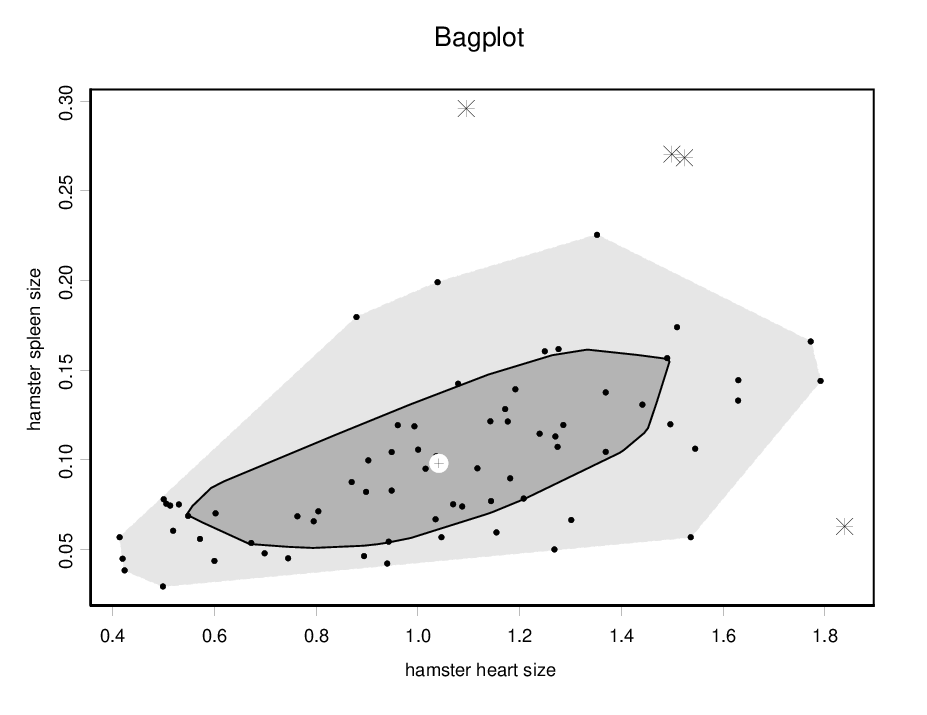
More generally, in the multivariate case one can define the bagdistance [24] of a point $\boldsymbol{x}$ relative to the Tukey median and the bag. Assume that the Tukey median lies in the interior of the bag, not on its boundary (this excludes degenerate cases). Then the bagdistance is the smallest real number $\lambda$ such that the bag inflated (or deflated) by $\lambda$ around the Tukey median contains the point $\boldsymbol{x}$. When the Tukey median equals $\boldsymbol{0}$, it is shown in [24] that the bagdistance satisfies all axioms of a norm except that $||a\boldsymbol{x}||=|a|||\boldsymbol{x}||$ only needs to hold when $a\geqslant 0$. The bagdistance is used for outlier detection [23] and statistical classification [24].

An often used criterion to judge the robustness of an estimator is its breakdown value. The breakdown value is the smallest fraction of data points that we need to replace in order to move the estimator of the contaminated data set arbitrarily far away. The classical mean of a data set has breakdown value zero since we can move it anywhere by moving one observation. Note that for any estimator which is equivariant for translation (which is required to call it a location estimator) the breakdown value can be at most 1/2. (If we replace half of the points by a far-away translation image of the remaining half, the estimator cannot distinguish which were the original data.)

The Tukey depth and the corresponding median have good statistical properties. The Tukey median $T^{*}$ is a location estimator with breakdown value $\varepsilon_{n}(T^{*};X_{n})$ $\geqslant 1/(d+1)$ for any data set in general position. This means that it remains in a predetermined bounded region unless $n/(d+1)$ or more data points are moved. At an elliptically symmetric distribution the breakdown value becomes 1/3 for large $n$, irrespective of $d$. Moreover, the halfspace depth is invariant under all nonsingular affine transformations of the data, making the Tukey median affine equivariant. Since data transformations such as rotation and rescaling are very common in statistics, this is an important property. The statistical asymptotics of the Tukey median have been studied in [4].

The need for fast algorithms for the halfspace depth has only grown over the years, since it is currently being applied to a variety of settings such as nonparametric classification [32]. A related development is the fast growing field of functional data analysis, where the data are functions on a univariate interval (e.g. time or wavelength) or on a rectangle (e.g. surfaces, images). Often the function values are themselves multivariate. One can then define the depth of a curve (surface) by integrating the depth over all points as in [12]. This functional depth can again be used for outlier detection and classification [23, 24], but it requires computing depths in many multivariate data sets instead of just one.

Remark: centerpoints. There is a close relationship between the Tukey depth and centerpoints, which have been long studied in computational geometry. In fact, Tukey depth extends the notion of centerpoint. A centerpoint is any point with halfspace depth $\geqslant\lceil n/(d+1)\rceil$. A consequence of Helly’s theorem is that there always exists at least one centerpoint, so the depth of the Tukey median cannot be less than $\lceil n/(d+1)\rceil$.

1. 1.

   Simplicial depth ([33]). The depth of $\boldsymbol{\theta}$ equals the number of simplices formed by $d+1$ data points that contain $\boldsymbol{\theta}$. Formally,

   $$sdepth(\boldsymbol{\theta};X_{n})=\#\{(i_{1},\ldots,i_{d+1});\boldsymbol{\theta}\in S[\boldsymbol{x}_{i_{1}},\ldots,\boldsymbol{x}_{i_{d+1}}]\}.$$

   The simplicial median is affine equivariant with a breakdown value bounded above by $1/(d+2)$. Unlike halfspace depth, its depth regions need not be convex.

2. 2.

   Oja depth ([43]). This is also called simplicial volume depth:

   $$odepth(\boldsymbol{\theta};X_{n})=\bigl(1+\sum_{(i_{1},\ldots,i_{d})}\ \{volume\ S[\boldsymbol{\theta},\boldsymbol{x}_{i_{1}},\ldots,\boldsymbol{x}_{i_{d}}]\}\bigr)^{-1}.$$

   The corresponding median is also affine equivariant, but has zero breakdown value.

3. 3.

   Projection depth. We first define the outlyingness ([14]) of any point $\boldsymbol{\theta}$ relative to the data set $X_{n}$ as

   $$O(\boldsymbol{\theta};X_{n})=\max_{\|\boldsymbol{u}\|=1}\frac{|\boldsymbol{u}^{\tau}\boldsymbol{\theta}-\med_{i}\{\boldsymbol{u}^{\tau}\boldsymbol{x}_{i}\}|}{\mbox{MAD}_{i}\{\boldsymbol{u}^{\tau}\boldsymbol{x}_{i}\}},$$

   where the median absolute deviation (MAD) of a univariate data set$\{y_{1},\ldots,y_{n}\}$ is the statistic $\mbox{MAD}_{i}\{y_{i}\}=\med_{i}|y_{i}-\med_{j}\{y_{j}\}|$. The outlyingness is small for centrally located points and increases if we move toward the boundary of the data cloud. Instead of the median and the MAD, also another pair $(T,S)$ of a location and scatter estimate may be chosen. This leads to different notions of projection depth, all defined as

   $$pdepth(\boldsymbol{\theta};X_{n})=(1+O(\boldsymbol{\theta};X_{n}))^{-1}.$$

   General projection depth is studied in [66]. When using the median and the MAD, the projection depth has breakdown value 1/2 and is affine equivariant. Its depth regions are convex.

4. 4.

   Spatial depth ([55]). Spatial depth is related to multivariate quantiles proposed in [9]:

   $$spdepth(\boldsymbol{\theta};X_{n})=1-\left\|\frac{1}{n}\sum_{i=1}^{n}\frac{\boldsymbol{x}_{i}-\boldsymbol{\theta}}{\|\boldsymbol{x}_{i}-\boldsymbol{\theta}\|}\right\|$$

   The spatial median is also called the $L^{1}$ median ([20]). It has breakdown value 1/2, but is not affine equivariant (it is only equivariant with respect to translations, multiplication by a scalar factor, and orthogonal transformations). For a recent survey on the computation of the spatial median see [19].

A comparison of the main properties of the different location depth medians is given in Table 1.

This notion of depth was originally defined ([46]) in the dual, as the depth of a regression hyperplane $H_{\boldsymbol{\theta}}$ relative to a point configuration of the form $Z_{n}=\{(\boldsymbol{x}_{1},y_{1}),\ldots,(\boldsymbol{x}_{n},y_{n})\}$ in $\mathbb{R}^{d+1}$. Regression depth ranks hyperplanes according to how well they fit the data in a regression model, with $\boldsymbol{x}$ containing the predictor variables and $y$ the response. A vertical hyperplane (given by $\boldsymbol{a}^{\tau}\boldsymbol{x}=$ constant), which cannot be used to predict future response values, is called a “nonfit” and assigned regression depth 0. The regression depth of a general hyperplane $H_{\boldsymbol{\theta}}$ is found by rotating $H_{\boldsymbol{\theta}}$ in a continuous movement until it becomes vertical. The minimum number of data points that is passed in such a rotation is called the regression depth of $H_{\boldsymbol{\theta}}$. Figure 4 is the dual representation of Figure 3. (For instance, the line $\boldsymbol{\theta}$ has slope $\theta_{1}$ and intercept $\theta_{2}$ and corresponds to the point $(\theta_{1},\theta_{2})$ in Figure 3.) The lines $\boldsymbol{\theta}$ and $\boldsymbol{\eta}$ have regression depth 0, whereas the line $\boldsymbol{\xi}$ has regression depth 2.

In statistics one is interested in the deepest fit or regression depth median, because this is a line (hyperplane) about which the data are well-balanced. The statistical properties of regression depth and the deepest fit are very similar to those of the Tukey depth and median. The bounds on the maximal depth are almost the same. Moreover, for both depth notions the value of the maximal depth can be used to characterize the symmetry of the distribution ([52]). The breakdown value of the deepest fit is at least $1/(d+1)$ and under linearity of the conditional median of $y$ given $\boldsymbol{x}$ it converges to 1/3. In the next section, we will see that the optimal complexities for computing the depth and the median are also comparable to those for halfspace depth. For a detailed comparison of the properties of halfspace and regression depth, see [22].

The arrangement depth region $D_{k}$ is defined in the primal, as the set of points with arrangement depth at least $k$. Contrary to the Tukey depth, these depth regions need not be convex. But nevertheless it was proved that there always exists a point with arrangement depth at least $\lceil n/(d+1)\rceil$ ([3]). An analysis-based proof was given in [39].

Remark: arrangement levels. Arrangement depth is undirected (isotropic) in the sense that it is defined as a minimum over all possible directions. If we restrict ourselves to vertical directions $\boldsymbol{u}$ (i.e., up or down), we obtain the usual levels of the arrangement known in combinatorial geometry. The absence of preferential directions makes arrangement depth invariant under affine transformations.

The algorithms for halfspace and simplicial depth are based on the same technique. First, data points are radially sorted around $\boldsymbol{\theta}$. Then a line through $\boldsymbol{\theta}$ is rotated. The depth is calculated by counting the number of points that are passed by the rotating line in a specific manner. The planar arrangement depth algorithm is easiest to visualize in the regression setting. To compute the depth of a hyperplane $H_{\boldsymbol{\theta}}$ with coefficients $\boldsymbol{\theta}$, the data are first sorted along the $x$-axis. A vertical line $L$ is then moved from left to right and each time a data point is passed, the number of points above and below $H_{\boldsymbol{\theta}}$ on both sides of $L$ is updated.

In general, computing a median is harder than computing the depth in a point, because typically there are many candidate points. For instance, for the bivariate simplicial median the currently best algorithm requires $O(n^{4})$ time, whereas its corresponding depth needs only $O(n\log n)$. The simplicial median seems difficult to compute because there are $O(n^{4})$ candidate points (namely, all intersections of lines passing through two data points) and the simplicial depth regions have irregular shapes, but of course a faster algorithm may yet be found.

Fortunately, in several important cases the median can be computed without computing the depth of individual points. A linear-time algorithm to compute a bivariate centerpoint was described in [25]. Table 3 gives an overview of algorithms to compute bivariate depth-based medians. For the bivariate Tukey median the lower bound $\Omega(n\log n)$ was proved in [28], and the currently fastest algorithm takes $O(n\log^{3}n)$ time ([30]). The lower bound $\Omega(n\log n)$ also holds for the median of arrangement (regression) depth as shown by [31]. Fast algorithms were devised by [31] and [63].

The computation of bivariate halfspace depth regions has also been studied. The first algorithm [53] required $O(n^{2}\log n)$ time per depth region. An algorithm to compute all regions in $O(n^{2})$ time is constructed and implemented in [38]. This algorithm thus also yields the Tukey median. It is based on the dual arrangement of lines where topological sweep is applied. A completely different approach is implemented in [27]. They make direct use of the graphics hardware to approximate the depth regions of a set of points in $O(nW+W^{3})+nCW^{2}/512$ time, where the pixel grid is of dimension $(2W+1)\times(2W+1)$. Recently, [8] constructed an algorithm to update halfspace depth and its regions when points are added to the data set.

For the computation of projection depth see [36]. The simplicial depth of a point in $\mathbb{R}^{3}$ can be computed in $O(n^{2})$ time, and in $\mathbb{R}^{4}$ the fastest algorithm needs $O(n^{4})$ time [11]. For higher dimensions, no better algorithm is known than the straightforward $O(n^{d+1})$ method to compute all simplices.

When the number of data points and dimensions are such that the above algorithms become infeasible, one can resort to approximate algorithms. For halfspace depth such approximate algorithms were proposed in [51] and [10]. An approximation to the Tukey median using steepest descent can be found in [60]. In [64] an algorithm is described to approximate the deepest regression fit in any dimension.

References

- [1] G. Aloupis, C. Cortés, F. Gómez, M. Soss, and G.T. Toussaint. Lower bounds for computing statistical depth. Comput. Stat. Data Anal., 40:223–229, 2002.
- [2] G. Aloupis, S. Langerman, M. Soss, and G.T. Toussaint. Algorithms for bivariate medians and a Fermat-Torricelli problem for lines. Comput. Geom. Theory Appl., 26:69–79, 2003.
- [3] N. Amenta, M. Bern, D. Eppstein, and S.-H. Teng. Regression depth and center points. Discrete Comput. Geom., 23:305–323, 2000.
- [4] Z.-D. Bai and X. He. Asymptotic distributions of the maximal depth estimators for regression and multivariate location. Ann. Statist., 27:1616–1637, 1999.
- [5] D. Bertsimas and R. Mazumder. Least quantile regression via modern optimization. Ann. Statist., 42:2494–2525, 2014.
- [6] D. Bremner, D. Chen, J. Iacono, S. Langerman, and P. Morin. Output-sensitive algorithms for Tukey depth and related problems. Stat. Comput., 18:259–266, 2008.
- [7] H. Brönnimann and B. Chazelle. Optimal slope selection via cuttings. Comput. Geom., 10:23–29, 1998.
- [8] M. Burr, E. Rafalin, and S.L. Souvaine. Dynamic maintenance of halfspace depth for points and contours. arXiv:1109.1517 (2011).
- [9] P. Chaudhuri. On a geometric notion of quantiles for multivariate data. J. Amer. Statist. Assoc., 91:862–872, 1996.
- [10] D. Chen, P. Morin, and U. Wagner. Absolute approximation of Tukey depth: theory and experiments. Comput. Geom., 46:566–573, 2013.
- [11] A.Y. Cheng and M. Ouyang. On algorithms for simplicial depth. In Proc. 13th Canadian Conf. on Comp. Geom., pages 53–56, Waterloo, 2001.
- [12] G. Claeskens, M. Hubert, L. Slaets, and K. Vakili. Multivariate functional halfspace depth. J. Amer. Statist. Assoc., 109:411–423, 2014.
- [13] M.B. Dillencourt, D.M. Mount, and N.S. Netanyahu. A randomized algorithm for slope selection. Internat. J. Comput. Geom. Appl., 2:1–27, 1992.
- [14] D.L. Donoho and M. Gasko. Breakdown properties of location estimates based on halfspace depth and projected outlyingness. Ann. Statist., 20:1803–1827, 1992.
- [15] R. Dyckerhoff and P. Mozharovskyi. Exact computation of the halfspace depth. arXiv:1411.6927 [stat.CO], 2014.
- [16] H. Edelsbrunner and D.L. Souvaine. Computing least median of squares regression lines and guided topological sweep. J. Amer. Statist. Assoc., 85:115–119, 1990.
- [17] D. Eppstein. Faster construction of planar two-centers. In Proc. 8th Annu. ACM-SIAM Sympos. Discrete Algorithms, pages 131–138, New Orleans, 1997.
- [18] D. Eppstein. Fast hierarchical clustering and other applications of dynamic closest pairs. In Proc. 9th Annu. ACM-SIAM Sympos. Discrete Algorithms, pages 619–628, San Francisco, 1998.
- [19] H. Fritz, P. Filzmoser, and C. Croux. A comparison of algorithms for the multivariate -median. Computation. Stat., 27:393–410, 2012.
- [20] J.C. Gower. The mediancenter. J. Roy. Statist. Soc. Ser. C, 32:466–470, 1974.
- [21] M. Hallin, D. Paindaveine, and M. Šiman. Multivariate quantiles and multiple-output regression quantiles: from -optimization to halfspace depth. Ann. Statist., 38:635–669, 2010.
- [22] M. Hubert, P.J. Rousseeuw, and S. Van Aelst. Similarities between location depth and regression depth. In L.T. Fernholz, editor, Statistics in Genetics and in the Environmental Sciences, pages 153–162. Birkhäuser Verlag, Basel, 2001.
- [23] M. Hubert, P.J. Rousseeuw, and P. Segaert. Multivariate functional outlier detection. Stat. Methods & Applic., 24:177–202, 2015.
- [24] M. Hubert, P.J. Rousseeuw, and P. Segaert. Multivariate and functional classification using depth and distance. arXiv:1504.01128, 2015.
- [25] S. Jadhav and A. Mukhopadhyay. Computing a centerpoint of a finite planar set of points in linear time. Discrete Comput. Geom., 12:291–312, 1994.
- [26] L. Kong and I. Mizera. Quantile tomography: using quantiles with multivariate data. Statistica Sinica, 22:1589–1610, 2012.
- [27] S. Krishnan, N.H. Mustafa, and S. Venkatasubramanian. Hardware-assisted computation of depth contours. In Proc. 13th Annu. ACM-SIAM Sympos. Discrete Algorithms, pages 558–567, 2002.
- [28] S. Langerman and W. Steiger. Computing a maximal depth point in the plane. In Proc. Japan Conf. on Discrete and Computational Geometry, pages 46–47, 2000.
- [29] S. Langerman and W. Steiger. An optimal algorithm for hyperplane depth in the plane. In Proc. 11th Annu. ACM-SIAM Sympos. Discrete Algorithms, pages 54–59, San Francisco, 2000.
- [30] S. Langerman and W. Steiger. Optimization in arrangements. Lecture Notes in Computer Science 2607, Springer-Verlag, Berlin, 2003.
- [31] S. Langerman and W. Steiger. The complexity of hyperplane depth in the plane. Discrete Comput. Geom., 30:299–309, 2003.
- [32] J. Li, J.A. Cuesta-Albertos, and R.Y. Liu. DD-classifier: nonparametric classification procedure based on DD-plot. J. Amer. Statist. Assoc., 107:737–753, 2012.
- [33] R.Y. Liu. On a notion of data depth based on random simplices. Ann. Statist., 18:405–414, 1990.
- [34] R.Y. Liu, J. Parelius, and K. Singh. Multivariate analysis by data depth: descriptive statistics, graphics and inference. Ann. Statist., 27:783–840, 1999.
- [35] X. Liu, K. Mosler, and P. Mozharovskyi. Fast computation of Tukey trimmed regions in dimension . arXiv:1412.5122 [stat.CO], 2014.
- [36] X. Liu and Y. Zuo. Computing projection depth and its associated estimators. Stat. Comput., 24:51–63, 2014.
- [37] J. Matoušek, D.M. Mount, and N.S. Netanyahu. Efficient randomized algorithms for the repeated median line estimator. Algorithmica, 20:136–150, 1998.
- [38] K. Miller, S. Ramaswami, P. Rousseeuw, J.A. Sellarès, D. Souvaine, I. Streinu, and A. Struyf. Efficient Computation of Location Depth Contours by Methods of Computational Geometry. Stat. Comput., 13:153–162, 2003.
- [39] I. Mizera. On depth and deep points: a calculus. Ann. Statist. 30:1681–1736, 2002.
- [40] K. Mosler. Depth statistics. In C. Becker, R. Fried, and S. Kuhnt, editors, Robustness and Complex Data Structures, pages 17–34, Springer-Verlag, Berlin Heidelberg, 2013.
- [41] D.M. Mount and N.S. Netanyahu. Computationally efficient algorithms for high-dimensional robust estimators. Graphical Models Image Proc., 56:289–303, 1994.
- [42] D.M. Mount, N.S. Netanyahu, K. Romanik, R. Silverman, and A.Y. Wu. A practical approximation algorithm for the LMS line estimator. In Proc. 8th Annu. ACM-SIAM Sympos. Discrete Algorithms, pages 473–482, New Orleans, 1997.
- [43] H. Oja. Descriptive statistics for multivariate distributions. Statist. Probab. Lett., 1:327–332, 1983.
- [44] S. Portnoy and R. Koenker. The Gaussian hare and the Laplacian tortoise: computability of squared-error versus absolute-error estimators. Stat. Sci., 12:279–300, 1997.
- [45] P.J. Rousseeuw. Least median of squares regression. J. Amer. Statist. Assoc., 79:871–880, 1984.
- [46] P.J. Rousseeuw and M. Hubert. Regression depth. J. Amer. Statist. Assoc., 94:388–402, 1999.
- [47] P.J. Rousseeuw and M. Hubert. Depth in an arrangement of hyperplanes. Discrete Comput. Geom., 22:167–176, 1999.
- [48] P.J. Rousseeuw and I. Ruts. Algorithm AS 307: Bivariate location depth. J. Roy. Statist. Soc. Ser. C, 45:516–526, 1996.
- [49] P.J. Rousseeuw and I. Ruts. Constructing the bivariate Tukey median. Statistica Sinica, 8:827-839, 1998.
- [50] P.J. Rousseeuw, I. Ruts, and J.W. Tukey. The bagplot: A bivariate boxplot. Amer. Statist., 53:382–387, 1999.
- [51] P.J. Rousseeuw and A. Struyf. Computing location depth and regression depth in higher dimensions. Stat. Comput., 8:193–203, 1998.
- [52] P.J. Rousseeuw and A. Struyf. Characterizing angular symmetry and regression symmetry. J. Statist. Plann. Inference, 122:161-–173, 2004.
- [53] I. Ruts and P.J. Rousseeuw. Computing depth contours of bivariate point clouds. Comput. Stat. Data Anal., 23:153–168, 1996.
- [54] P.K. Sen. Estimates of the regression coefficient based on Kendall’s tau. J. Amer. Statist. Assoc., 63:1379–1389, 1968.
- [55] R. Serfling. A depth function and a scale curve based on spatial quantiles. In Y. Dodge, editor, Statistical Data Analysis Based on the L1-Norm and Related Methods, pages 25–38, Birkhaüser, Basel, 2002.
- [56] M.I. Shamos. Geometry and statistics: problems at the interface. In J.F. Traub, editor, Algorithms and Complexity: New Directions and Recent Results, pages 251–280. Academic Press, Boston, 1976.
- [57] A. Siegel. Robust regression using repeated medians. Biometrika, 69:242–244, 1982.
- [58] C.G. Small. A survey of multidimensional medians. Internat. Statistical Review, 58:263–277, 1990.
- [59] A. Struyf, M. Hubert, and P.J. Rousseeuw. Integrating robust clustering techniques in S-PLUS. Comput. Stat. Data Anal., 26:17–37, 1997.
- [60] A. Struyf and P.J. Rousseeuw. High-dimensional computation of the deepest location. Comput. Stat. Data Anal., 34:415–426, 2000.
- [61] H. Theil. A rank-invariant method of linear and polynomial regression analysis (parts 1-3). Nederl. Akad. Wetensch. Ser. A, 53:386–392, 521–525, 1397–1412, 1950.
- [62] J.W. Tukey. Mathematics and the picturing of data. In Proc. Internat. Congr. of Math., 2, pages 523–531, Vancouver, 1975.
- [63] M. van Kreveld, J. Mitchell, P. Rousseeuw, M. Sharir, J. Snoeyink, B. Speckmann. Efficient algorithms for maximum regression depth. Discrete Comput. Geom., 39:656–677, 2008.
- [64] S. Van Aelst, P.J. Rousseeuw, M. Hubert, and A. Struyf. The deepest regression method. J. Multivar. Anal., 81:138–166, 2002.
- [65] P. Yamamoto, K. Kato, K. Imai, and H. Imai. Algorithms for vertical and orthogonal linear approximation of points. In Proc. 4th Sympos. Comput. Geom., pages 352–361, 1988.
- [66] Y. Zuo. Projection based depth functions and associated medians. Ann. Statist., 31:1460–1490, 2003.
- [67] Y. Zuo and R. Serfling. General notions of statistical depth function. Ann. Statist., 28:461–482, 2000.