Maxwell’s Demon Based on a Single Qubit

Controllable small systems, e.g. in form of molecules, micro-beads or nanoelectronic circuits [1, 2, 3, 4, 5, 6], have recently made it possible to experiment on thermodynamics in the regime where fluctuations play an important role. One of the most interesting issues in such stochastic thermodynamics is the role of information. On the level of thought experiments this discussion dates back all the way to Maxwell’s demon (MD) [7] and then to Landauer’s principle [8]. Till now, majority of the studies, both theoretically and in particular experimentally [9, 10, 11, 12], have been focusing on the classical regime; see, however, [13, 14, 15, 16, 17] and references therein for theories on quantum systems. The aim of this Letter is to present a simple and experimentally feasible quantum MD that can operate at the limit of thermodynamic efficiency. Demon operation is based on a qubit, a two-level system (TLS) with avoided level crossing between the ground ($g$) and the excited ($e$) state as illustrated in Fig. 1. The TLS is coupled weakly to a bath at temperature $T$. The MD moves around the level crossing by tuning the control parameter $q$.

We first present an ideal operation cycle and results for the MD without justifying their feasibility. The cycle start at point A in Fig. 1, where the level separation $\Delta E$ is maximum denoted by $\Delta E_{A}$. If $\Delta E_{A}\gg k_{B}T$, the system is in the ground state with zero entropy. In the first leg, $q$ is moved adiabatically to the point X with minimum level spacing $\Delta E_{0}$. We assume that the ramps are linear in time, i.e. $\dot{q}={\rm constant}$ within each leg. Ideally, for $\Delta E_{0}\ll k_{B}T$ and fully adiabatical ramp, the entropy of the TLS increases by $k_{B}\ln 2$, corresponding to heat extracted from the bath equal to Landauer value $Q_{L}=k_{B}T\ln 2$. This part of the cycle is equivalent to that in a classical TLS – see Ref. [11], although the non-vanishing $\Delta E_{0}$ creates essential differences in the quantum regime. On reaching point X, a measurement of the qubit state is performed. If the detector measures the appropriate quantity: the energy or the curvature $d^{2}E/dq^{2}$ (which, depending on the physical realization of the system can represent, e.g., effective capacitance or inductance in an electric circuit) it does not perturb this state and therefore, does not incur any thermodynamic costs. Note that, in contrast to a classical MD, the possibility to realize such a measurement required for the thermodynamically efficient quantum MD, is not automatic, but relies on the feature of adiabatic dynamics to leave the qubit density matrix diagonal in the energy basis. After the measurement, the detector, ideally, “knows” with certainty whether the system is in the ground state or in the excited state in each cycle. In the repeated cycles, the two states are realized with equilibrium thermal probabilities. This makes it possible to apply conditional feedback: if the system is in the ground state, the control gate is moved quickly back to the original position. In the excited state, a $\pi$-pulse is applied to the qubit swapping the state $e\rightarrow g$, the process in which the work done by the source is $-\Delta E_{0}$ [18, 19], followed again by a fast ramp in the ground state back to the original position A. Extracted heat, averaged over several such ideal cycles is

where $\beta=(k_{B}T)^{-1}$.

Several processes can compromise the ideal performance of the qubit demon. First, one may extract less heat from the bath if the ramp A $\rightarrow$ X is not fully adiabatic. Also, the feedback ramp X $\rightarrow$ A needs to be “fast” to avoid bath-induced transitions but “slow” to avoid Landau-Zener excitation out of the ground state. Both processes would create extra dissipation. To consider them quantitatively, we start with the operator of the power injected into the system, $P(t)=\dot{H}(t)$, where $H(t)$ is the system Hamiltonian. Work $W$ done on the system over a time interval $\tau$ is then $W=\int_{0}^{\tau}P(t)dt$. Since we are mainly interested in quantities averaged over many cycles, it is convenient to describe the dynamics with the density matrix $\rho(t)$. For average work $\langle W\rangle=\langle\int_{0}^{\tau}P(t)dt\rangle$ one finds by elementary analysis [20]

Equation (2) represents the first law of thermodynamics, combining the change of the internal energy and the average heat generated in the bath: $\langle Q\rangle=-\int_{0}^{\tau}{\rm Tr}\big[\dot{\rho}(t)H(t)\big]dt$. In the basis $\{|g\rangle,|e\rangle\}$ of instantaneous eigenstates of the qubit, this expression gives

The standard master equation for the qubit density matrix $\rho(t)$, ignoring pure dephasing, is

where $\Omega=\frac{\epsilon}{q^{2}+\epsilon^{2}}\dot{q}$ depends on the ramp rate of $q$, $\epsilon=\Delta E_{0}/(2\Delta E_{A})$, and the level spacing is $\Delta E(t)=2\Delta E_{A}\sqrt{q(t)^{2}+\epsilon^{2}}$. Point A corresponds to $q=-1/2$, whereas point X is at $q=0$. The relaxation and excitation rates of the qubit are, respectively,

and $\Gamma_{\Sigma}=\Gamma_{\downarrow}+\Gamma_{\uparrow}$. Parameter $g^{2}$ denotes the dimensionless strength of coupling to the bath.

To learn about stochastics beyond the averages above, we analyze quantum trajectories corresponding to the master equation (4) for the evolution of the wave function $|\psi(t)\rangle=a(t)|g\rangle+b(t)|e\rangle$. According to the quantum jump approach [21], the probability to relax to $|g\rangle$ (get excited to $|e\rangle$) over a short time interval $\Delta t$ is given by $\Delta p_{\downarrow}=\Gamma_{\downarrow}|b(t)|^{2}\Delta t$ ($\Delta p_{\uparrow}=\Gamma_{\uparrow}|a(t)|^{2}\Delta t$). If such a jump does not occur, the system evolves as

where $\Delta\Gamma(t)=\Gamma_{\downarrow}(t)-\Gamma_{\uparrow}(t)=g^{2}\Delta E(t)/\hbar$. The evolution of the system is obtained numerically using a stochastic simulation based on these equations. The heat dissipated into the bath is given by $(-)\Delta E$ when the system relaxes (gets excited) [22], see also [23].

We analyze the MD cycle and errors quantitatively assuming that the measurement and the conditional $\pi$-pulse are fast enough (duration $\ll\Gamma_{\Sigma}^{-1}$) so that no heat is exchanged in this time interval. Consider first the quasi-static sweep A $\rightarrow$ X in time $\tau=(2\dot{q})^{-1}$. For $\tau\rightarrow\infty$, the population obeys

according to Eq. (4). Inserting this expression into Eq. (3), we obtain

Assuming everywhere below that $\beta\Delta E_{A}\gg 1$, we recover Eq. (1). If $\Delta E_{0}=0$, we obtain then the most familiar result $\langle Q\rangle=-k_{B}T\ln 2=-Q_{L}$. For such a degenerate case, the average heat equals the heat obtained in each adiabatic realization, but this is not so for $\Delta E_{0}>0$.

For finite values of $\tau$, the evolution becomes non-adiabatic and can be analyzed using Eq. (4). Provided $\hbar/(2\pi\epsilon^{2}\Delta E_{A}\tau)\ll 1$, one can neglect Zener tunneling processes and set $\Omega=0$ in Eq. (4). Then one finds exactly

In Fig. 2, we present results on $\langle Q\rangle$ normalized by $k_{B}T$ as a function of the ramping rate $v=\hbar/(2\tau\Delta E_{A})$ in the A $\rightarrow$ X ramp for chosen parameters. The black line is based on the master equation (4) together with (3), and is indistinguishable from Eq. (9). The blue symbols are from the stochastic simulation with $50000$ repetitions for each point. The horizontal arrow indicates the adiabatic result of Eq. (1).

The errors in the fast return ramp X $\rightarrow$ A in time $\tau_{R}$ are produced by the Landau-Zener processes which generate finite population of the excited state. If the excited state amplitude is $b_{f}$ at the end of the sweep, there is “quantum” heat $\sim|b_{f}|^{2}\Delta E_{A}$ dissipated into the bath in the next adiabatic ramp to $q=0$. On the other hand, if the sweep is too slow and $\Gamma_{\uparrow}\tau_{R}\ll 1$ does not hold, the system can be excited by the bath, and there is extra “classical” generated heat when the system relaxes either before or during the adiabatic ramp in the next cycle. These two errors constrict the ramp time to the interval $\hbar/(\epsilon^{2}\Delta E_{A})\ll\tau_{R}\ll\Gamma_{\uparrow}^{-1}$ as a condition of approaching the ideal operation. The lower bound is the same as for the standard Landau-Zener dynamics.

We estimate these two contributions to heat as follows. For weak dissipation and system being mostly in the ground state, we write the evolution of $b$ as (see (6)) $\dot{b}\approx\frac{1}{2}\Omega e^{+i\int_{0}^{t}\Delta E(t^{\prime})dt^{\prime}/\hbar}$. Linearizing the expression in the exponent with respect to $q$, and denoting the dimensionless rate as $v_{R}=\hbar/(2\tau_{R}\Delta E_{A})$, we obtain the final population at the end of the ramp as

valid for $|b_{f}|^{2}\ll 1$. This result agrees with the one obtained in [24].

The corresponding classical error is determined by the probability $p_{\uparrow}$ of a thermal excitation $g\rightarrow e$ during the ramp, again assuming that $|a|^{2}\approx 1$. This yields

Both excitation processes, described by Eqs. (10) and (11), combine to produce extra average heat dissipated in a cycle: $\langle Q_{\rm diss}\rangle\approx(|b_{f}|^{2}+p_{\uparrow})\Delta E_{A}$. Minimum of $\langle Q_{\rm diss}\rangle$,

with respect to $v_{R}$ is then obtained at

In this optimization, we considered only the most straightforward linear return ramp, for which the excitation amplitude $b_{f}$ (10) decreases as $1/\tau_{R}$. In principle, $b_{f}$ can be suppressed more strongly if the return ramp is switched not abruptly, as in the cycles considered above, but smoothly. As discussed in the Supplementary Material [25], the amplitude $b_{f}$ decreases as $(\hbar/\Delta E_{0}\tau_{R})^{n}$, if only the $n$th-order derivative of the switching function is discontinuous, while all previous derivatives are continuous, and exponentially, if the switching function has continuous derivatives of any order.

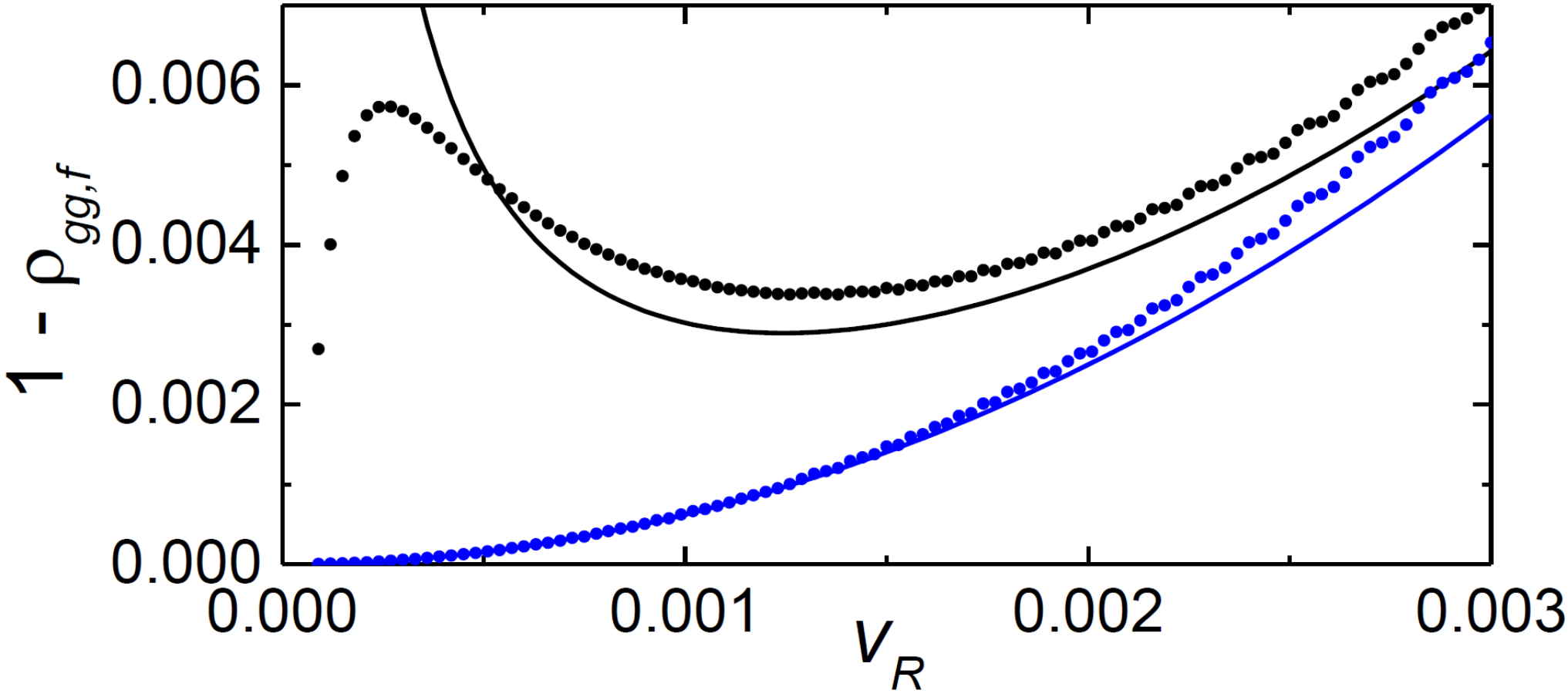
The approximations above are shown together with full master equation solutions in Fig. 3, again for $\epsilon=0.1$ and $\beta\Delta E_{A}=10$ for the ramp X $\rightarrow$ A as a function of the sweep rate $v_{R}$ for two cases of $g^{2}=10^{-3}$ and $g^{2}=0$. The predictions based on the analytical estimates, i.e. $1-\rho_{gg,f}=|b_{f}|^{2}+p_{\uparrow}$ are shown by black and blue lines for the two values of $g^{2}$, respectively. The corresponding solutions based on the master equation are shown by solid symbols for the two values of $g^{2}$ as well. We see that the approximations are relatively accurate in this regime. The decline for $v_{R}\rightarrow 0$ of the master equation data set for $g^{2}=10^{-3}$ (black dots) is due to relaxation back from the excited state, the effect ignored in the analytical estimates.

As the last step of the numerical analysis of the demon, we have performed simulations based on the quantum trajectory method in cyclic operation. In this situation, once a cycle has finished, the state of the qubit when reaching point A serves as a new initial state of the next adiabatic ramp A $\rightarrow$ X. Thus, dynamics of the previous return path makes the initial state not necessarily the ground state, which leads to extra dissipation. Figure 4 shows results of this analysis, where heat accumulation over $N$ cycles up to $N=10^{4}$ has been analyzed under different driving parameters. In all these simulations, $\epsilon=0.1$, $\beta\Delta E_{A}=10$, and $g^{2}=10^{-3}$. In Fig. 4 (a), the rate of return sweep remains constant, at $v_{R}=1.25\cdot 10^{-3}$, which is close to its optimum value. The parameter indicated within the figure is the ramp rate $v$ of the adiabatic leg. We see clear cooling by the MD and correspondence with Fig. 2. For comparison, the fast rising (red) line indicates results of the calculation where the parameters are as for the lowest black curve in the figure, but without the measurement and $\pi$-pulse before the ramp back to A. This protocol is similar to a periodically driven two level system, which has been studied in detail recently [26, 27]. Naturally in such deterministic cycles there is positive heat dissipated into the bath according to the second law. The lowest (blue) line shows the result of Eq. (1) which would be achieved if the first ramp were fully adiabatic, and the system would remain constantly in the ground state during the return leg. In Fig. 4 (b) we show similar data as in (a), but now keeping the adiabatic ramp at a constant rate $v=10^{-6}$. The return rate $v_{R}$ is in turn varied here. We see correspondence with Fig. 3, showing the optimum rate of about $v_{R}=1.25\cdot 10^{-3}$.

It is possible to make some general statements as to the thermodynamic efficiency of the considered quantum MD. Thermodynamic cost of information acquired by the detector, based on Landauer’s principle, is $-k_{B}T(\rho_{gg}\ln\rho_{gg}+\rho_{ee}\ln\rho_{ee})$, where $\rho_{ee}=1-\rho_{gg}$. For ideal cycles considered above, this cost equals the heat $|\langle Q\rangle|$ of Eq. (1) extracted in a cycle. In this respect, ideally, the presented MD is fully reversible. Work $W_{\pi}$ done in applying the $\pi$-pulse can obtain two values, $W_{\pi}=0$ if the system is in the ground state and nothing is done, or $W_{\pi}=-\Delta E_{0}$ if the two-level system is in the excited state and the pulse is indeed applied. Therefore, averaging over many cycles, we obtain

Inserting Eq. (1) for average heat, we find that

Both $\langle W_{\pi}\rangle$ and $\langle Q\rangle$ are negative. Thus the work extraction in this step is less than the heat extraction in the whole cycle. In steady state, the average work in the whole cycle $\langle W\rangle=\langle Q\rangle$ according to Eq. (2), see also [25].

Finally, a few words about experimental feasibility of the proposed qubit demon. The principle studied here applies naturally to a large variety of systems, including solid-state qubits. As a concrete example, we may consider a superconducting qubit, e.g., a charge qubit [28, 29] or transmon qubit [29, 30]. Typical energy scale in this case is $\Delta E_{A}/k_{B}\sim 1$ K, as aluminium, the most common superconductor in this respect, has an energy gap $\Delta/k_{B}\approx 2$ K. Since the operating (bath) temperature of these devices is $T\sim 100$ mK, we indeed have $\beta\Delta E_{A}\sim 10$, as in the numerical examples above. In a charge-type qubit, $\epsilon$ is the ratio of the Josephson coupling and capacitive charging energies, and can be made to be $\sim 0.1$, based on design and tuning by magnetic flux. The value of $g^{2}=10^{-3}$ would correspond to a relaxation time of the qubit, $T_{1}=1/\Gamma_{\Sigma}$, which is then in the range $0.1...1$ $\mu$s, quite feasible for the current technology. The ramp times for the demon fall also in a favourable regime. Since $\tau\sim 10^{5}\hbar/\Delta E_{A}\sim 1$ $\mu$s yields still about 80% efficiency in the adiabatic leg as compared to the infinitely slow ramp (see Fig. 2), we may take this as a naive trade-off value in terms of efficiency vs. power extraction. The duration of the whole cycle is determined almost entirely by $\tau$. It is interesting to see that 1 $\mu$s is about 100 times faster than a typical electron-phonon relaxation time at these low temperatures [31, 32]. Therefore, if the bath is composed of, e.g., a micron-scale metallic calorimeter, it is reasonable to expect that the steady-state temperature of this absorber would decrease once the MD is set into cyclic operation [32]. Measuring this temperature drop would serve as a smoking gun of the proof of the principle of the demon. Last, we found that $\tau_{R}\sim 10^{3}\hbar/\Delta E_{A}\sim 10$ ns would be optimal with these parameters of the MD. This again is fully compatible with the time scales of the gate and flux operations of superconducting qubits.

The work has been supported by the European Union FP7 project INFERNOS (grant agreement 308850) and by the Academy of Finland (projects 272218 and 284594). D.V.A. was also supported in part by the NSF grant PHY-1314758.

References

- [1] C. Bustamante, J. Liphardt, and F. Ritort, Phys. Today 58, 43 (2005).
- [2] T. B. Batalhao, A. M. Souza, L. Mazzola, R. Auccaise, R. S. Sarthour, I. S. Oliveira, J. Goold, G. De Chiara, M. Paternostro, and R. M. Serra, Phys. Rev. Lett. 113, 140601 (2014).
- [3] S. Ciliberto, S. Joubaud, and A. Petrosyan, J. Stat. Mech. P12003 (2010).
- [4] V. Blickle, T. Speck, L. Helden, U. Seifert, and C. Bechinger, Phys. Rev. Lett. 96, 070603 (2006).
- [5] B. Küng, C. Rössler, M. Beck, M. Marthaler, D. S. Golubev, Y. Utsumi, T. Ihn, and K. Ensslin, Phys. Rev. X 2, 011001 (2012).
- [6] O.-P. Saira, Y. Yoon, T. Tanttu, M. Möttönen, D. V. Averin and J. P. Pekola, Phys. Rev. Lett. 109, 180601 (2012).
- [7] Maxwell’s Demon, ed. by H.S. Leff and A.F. Rex, (IOP Publishing, 2003).
- [8] R. Landauer, IBM J. Res. Develop. 5, 183191 (1961).
- [9] S. Toyabe, T. Sagawa, M. Ueda, E. Muneyuki, and M. Sano, Nat. Phys. 6, 988 (2010).
- [10] A. Berut, A. Arakelyan, A. Petrosyan, S. Ciliberto, R. Dillenschneider, and E. Lutz, Nature 483, 187 (2012).
- [11] J. V. Koski, V. F. Maisi, J. P. Pekola, and D. V. Averin, Proc. Natl. Acad. Sci. 111, 13786 (2014).
- [12] E. Roldan, I. A. Martinez, J. M. R. Parrondo, and D. Petrov, Nat. Phys. 10, 457 (2014).
- [13] S. Lloyd, Phys. Rev. A 56, 3374 (1997).
- [14] H. T. Quan, Y. D. Wang, Yu-xi Liu, C. P. Sun, and F. Nori, Phys. Rev. Lett. 97, 180402 (2006).
- [15] J. M. Horowitz and K. Jacobs, Phys. Rev. E 89, 042134 (2014).
- [16] K. Brandner, M. Bauer, M. T. Schmid, and U. Seifert, New J. Phys. 17, 065006 (2015).
- [17] J. M. R. Parrondo, J. M. Horowitz, and T. Sagawa, Nat. Phys. 11, 131 (2015).
- [18] P. Talkner, E. Lutz, and P. Hänggi, Phys. Rev. E 75, 050102(R) (2007).
- [19] M. Esposito, U. Harbola, and S. Mukamel, Rev. Mod. Phys. 81, 1665 (2009).
- [20] P. Solinas, D. V. Averin, and J. P. Pekola, Phys. Rev. B 87, 060508(R) (2013).
- [21] J. Dalibard, Y. Castin, and K. Mölmer, Phys. Rev. Lett. 68, 580 (1992).
- [22] F. W. J. Hekking and J. P. Pekola, Phys. Rev. Lett. 111, 093602 (2013).
- [23] J. M. Horowitz and J. M. R. Parrondo, New J. Phys. 15, 085028 (2013).
- [24] F. M. Cucchietti, B. Damski, J. Dziarmaga, and W. H. Zurek, Phys. Rev. A 75, 023603 (2007).
- [25] See Supplemental Material of this article.
- [26] P. Wollfarth, A. Shnirman, and Y. Utsumi, Phys. Rev. B 90, 165411 (2014).
- [27] S. Gasparinetti, P. Solinas, A. Braggio, and M. Sassetti, New J. Phys. 16, 115001 (2014).
- [28] D.V. Averin, Solid State Commun. 105, 659 (1998).
- [29] Y. Nakamura, Y. A. Pashkin, and J. S. Tsai, Nature 398, 786 (1999).
- [30] J. Koch, T. M. Yu, J. Gambetta, A. A. Houck, D. I. Schuster, J. Majer, A. Blais, M. H. Devoret, S. M. Girvin, and R. J. Schoelkopf, Phys. Rev. A 76, 042319 (2007).
- [31] L. J. Taskinen, J. M. Kivioja, J. T. Karvonen, and I. J. Maasilta, phys. stat. sol. (c) 1, 2856 (2004).
- [32] S. Gasparinetti, K.L. Viisanen, O.-P. Saira, T. Faivre, M. Arzeo, M. Meschke, and J. P. Pekola, Phys. Rev. Applied 3, 014007 (2015).
I Appendix I: Suppression of the Landau-Zener processes by smooth drive
In this Section of the Supplementary Material, we provide a brief discussion of the effect of smooth drive on the amplitude of the Landau-Zener excitation of the qubit out of the ground state in the process of rapid ramp back from the level-crossing point to the initial state. The most basic ramp-back process studied in the main text is characterized by the time dependence of the control parameter , which is continuous itself, but has discontinuous first derivative: for (we take the instant of measurement and, when needed, the -pulse, to be ) and for . This discontinuity of the first derivative leads to the excitation amplitude which decreases as with the ramp time – see Eq. (10) of the main text. The point of our discussion here is to demonstrate that the amplitude can be made to decrease faster with the ramp time , if any discontinuities of the time dependence of the control parameter at the point where the ramp is switched on, are suppressed more strongly. The statement that we want to make here, demonstrated by examples, is that the amplitude can be made to decreases as , if the switching function is such that only its th-order derivative is discontinuous, while all previous derivatives are continuous, and exponentially, if has continuous derivatives of any order.
To do this, we need to calculate the excitation probability for evolution starting at the level-crossing point. For the part of the MD cycle, ramp back to the initial state, which is considered in this discussion, we are interested in the regime of sufficiently slow time evolution, when the probability is small, i.e., the qubit stays predominantly in the ground state. On the other hand, this ramp of the control parameter should be fast enough for the thermal-bath-induced transitions to be negligible in the calculation of . As follows from Eq. (6) of the main text, in this regime, the evolution equation of the excitation amplitude is