跳到论文正文
W Papers独立论文阅读器 arXiv:1508.03783 论文正文 计算阅读时间 · 0%
引用这篇论文根据当前论文元数据生成,正式投稿前建议核对。


License: arXiv.org perpetual non-exclusive license
arXiv:1508.03783v3 [math.NA] 13 Sep 2015

Convergence rate for a Radau collocation method applied to unconstrained optimal control Thanks:  August 17, 2015. Revised September 12, 2015. The authors gratefully acknowledge support by the Office of Naval Research under grants N00014-11-1-0068 and N00014-15-1-2048, and by the National Science Foundation under grants DMS-1522629 and CBET-1404767.

William W. Hager ††thanks: hager@ufl.edu, http://people.clas.ufl.edu/hager/, PO Box 118105, Department of Mathematics, University of Florida, Gainesville, FL 32611-8105. Phone (352) 294-2308. Fax (352) 392-8357.    Hongyan Hou ††thanks: hongyan388@gmail.com, Chemical Engineering, Carnegie Mellon University, 5000 Forbes Avenue, Pittsburgh, PA 15213.    Anil V. Rao ††thanks: anilvrao@ufl.edu, http://www.mae.ufl.edu/rao Department of Mechanical and Aerospace Engineering, P.O. Box 116250, Gainesville, FL 32611-6250. Phone:(352) 392-0961. Fax:(352) 392-7303
Abstract

A local convergence rate is established for an orthogonal collocation method based on Radau quadrature applied to an unconstrained optimal control problem. If the continuous problem has a sufficiently smooth solution and the Hamiltonian satisfies a strong convexity condition, then the discrete problem possesses a local minimizer in a neighborhood of the continuous solution, and as the number of collocation points increases, the discrete solution convergences exponentially fast in the sup-norm to the continuous solution. An earlier paper analyzes an orthogonal collocation method based on Gauss quadrature, where neither end point of the problem domain is a collocation point. For the Radau quadrature scheme, one end point is a collocation point.

keywords
Radau collocation method, convergence rate, optimal control, orthogonal collocation

1 Introduction

A convergence rate is established for an orthogonal collocation method applied to an unconstrained control problem of the form

minimizeC⁡(𝐱⁡(1))subject to𝐱˙​(t)=𝐟⁡(𝐱⁡(t),𝐮⁡(t)),t∈[−1,1],𝐱⁡(−1)=𝐱0,\begin{array}[]{clc}\mbox{minimize}&C({\bf{x}}(1))&\\ \mbox{subject to}&\dot{{\bf{x}}}(t)={\bf{f(x}}(t),{\bf{u}}(t)),&t\in[-1,1],\\ &{\bf{x}}(-1)={\bf{x}}_{0},&\end{array} (1)

where the state 𝐱⁡(t)∈ℝn{{\bf{x}}}(t)\in\mathbb{R}^{n}, 𝐱˙≡dd​t​𝐱\dot{{\bf{x}}}\equiv\displaystyle\frac{d}{dt}{{\bf{x}}}, the control 𝐮⁡(t)∈ℝm{{\bf{u}}}(t)\in{\mathbb{R}}^{m}, 𝐟:ℝn×ℝm→ℝn{{\bf{f}}}:{\mathbb{R}}^{n}\times{\mathbb{R}}^{m}\rightarrow{\mathbb{R}}^{n}, C:ℝn→ℝC:{\mathbb{R}}^{n}\rightarrow{\mathbb{R}}, and 𝐱0{{\bf{x}}}_{0} is the initial condition, which we assume is given. Assuming the dynamics 𝐱˙​(t)=𝐟⁡(𝐱⁡(t),𝐮⁡(t))\dot{{\bf{x}}}(t)={\bf{f(x}}(t),{\bf{u}}(t)) is nice enough, we can solve for the state 𝐱{\bf{x}} as a function of the control 𝐮{\bf{u}}, and the control problem reduces to an unconstrained minimization over 𝐮{\bf{u}}.

Let 𝒫N{\cal{P}}_{N} denote the space of polynomials of degree at most NN defined on the interval [−1,+1][-1,+1], and let 𝒫Nn{\cal{P}}_{N}^{n} denote the nn-fold Cartesian product 𝒫N×…×𝒫N{\cal{P}}_{N}\times\ldots\times{\cal{P}}_{N}. We analyze a discrete approximation to (1), introduced in [11, 12], of the form

minimizeC⁡(𝐱⁡(1))subject to𝐱˙(τi)=𝐟(𝐱(τi),𝐮i),1≤i≤N,𝐱(−1)=𝐱0,𝐱∈𝒫Nn.\begin{array}[]{cl}\mbox{minimize}&C({\bf{x}}(1))\\ \mbox{subject to}&\dot{{\bf{x}}}(\tau_{i})={\bf{f(x}}(\tau_{i}),{\bf{u}}_{i}),\quad 1\leq i\leq N,\\ &{\bf{x}}(-1)={\bf{x}}_{0},\quad{\bf{x}}\in{\cal{P}}_{N}^{n}.\end{array} (2)

At the collocation points τi\tau_{i}, 1≤i≤N1\leq i\leq N, the equation should be satisfied. The control approximation at time τi\tau_{i} is 𝐮i{\bf{u}}_{i}. We focus on the Radau quadrature points satisfying

−1<τ1<τ2<…<τN=+1.-1<\tau_{1}<\tau_{2}<\ldots<\tau_{N}=+1.

The analysis we give also applies to the flipped Radau scheme obtained by reversing the sign for each collocation point. In (2) the dimension of 𝒫N{\cal{P}}_{N} is N+1N+1, while there are N+1N+1 equations in (2) corresponding to the collocated dynamics at NN points and the initial condition. When the discrete dynamics is nice enough, we can solve for the discrete state 𝐱∈𝒫Nn{\bf{x}}\in{\cal{P}}_{N}^{n} as a function of the discrete controls 𝐮i{\bf{u}}_{i}, 1≤i≤N1\leq i\leq N, and the discrete approximation reduces to an unconstrained minimization over the discrete controls.

In an earlier paper [16] we analyzed a scheme based on Gauss quadrature, where the collocation points lie in the interior of the interval [−1,+1][-1,+1]. The Gauss scheme is easier to analyze than the Radau scheme of this paper due to the symmetry of the Gauss collocation points, and the fact that the none of the collocation points lies at an end of the problem domain. For the Radau scheme, symmetry is broken and the polynomials in the discrete adjoint equation have degree N−1N-1 compared to the degree NN polynomials used for the state approximation. As will be seen, the presence of the Radau collocation point at the end of the interval [−1,+1][-1,+1] leads to the embedding of the terminal adjoint condition of the discrete problem into the discrete adjoint dynamics. Despite these differences in the analysis and despite the fact that Gauss quadrature has a higher degree of accuracy than Radau quadrature, the convergence rate obtained for the Radau scheme is exactly the same as that of the Gauss scheme. Moreover, in numerical experiments with test problems where an exact solution is known, the observed error in the state, control, and adjoint for the Radau scheme is very similar to the observed error for the Gauss scheme. The fact that a Radau quadrature point can be placed at the end point of the interval leads to a simpler implementation of terminal constraints and terminal cost. And the Radau scheme is easier than the Gauss scheme to extend to an h​php-framework [1, 2, 20, 22] where the interval [−1,+1][-1,+1] is partitioned into a mesh and a different polynomial is employed in each mesh interval.

The analysis in this and the earlier paper [16] needs further extensions in order to handle Lobatto collocation schemes such as those in [7, 9] where τ1=−1\tau_{1}=-1 and τN=+1\tau_{N}=+1. Although the Gauss and Radau scheme have similar errors, the Lobatto scheme can converge at a slower rate, as observed in [12]. An advantage of the Lobatto scheme is that the value of the optimal control is estimated at the initial point t=−1t=-1 and the terminal point t=+1t=+1. Moreover, both initial and terminal constraints are easier to implement in the Lobatto framework. A consistency result for a Lobatto collocation scheme applied to optimal control is given in [13]. Other quadrature points that have been exploited in the optimal control literature include the Chebyshev quadrature points [8, 10], and the extrema of Jacobi polynomials [26].

Our goal is to show that if (𝐱∗,𝐮∗)({\bf{x}}^{*},{\bf{u}}^{*}) is a local minimizer for (1), then the discrete problem (2) has a local minimizer (𝐱N,𝐮N)({\bf{x}}^{N},{\bf{u}}^{N}) that converges exponentially fast in NN to (𝐱∗,𝐮∗)({\bf{x}}^{*},{\bf{u}}^{*}) at the collocation points. Convergence rates have been obtained previously when the approximating space consists of piecewise polynomials as in [3, 4, 6, 5, 14, 19, 23]. In these earlier results, convergence is achieved by letting the mesh spacing tend to zero. In our results, on the other hand, convergence is achieved by letting NN, the degree of the approximating polynomials, tend to infinity.

Let 𝒞k​(ℝn){\cal{C}}^{k}(\mathbb{R}^{n}) denote the space of kk times continuously differentiable functions 𝐱:[−1,+1]→ℝn{\bf{x}}:[-1,+1]\rightarrow\mathbb{R}^{n} with the sup-norm ∥⋅∥∞\|\cdot\|_{\infty} given by

‖𝐱‖∞=sup{|𝐱⁡(t)|:t∈[−1,+1]},\|{\bf{x}}\|_{\infty}=\sup\{|{\bf{x}}(t)|:t\in[-1,+1]\}, (3)

where |⋅||\cdot| is the Euclidean norm. It is assumed that (1) has a local minimizer (𝐱∗,𝐮∗)({\bf{x}}^{*},{\bf{u}}^{*}) in 𝒞1​(ℝn)×𝒞0​(ℝm){\cal{C}}^{1}(\mathbb{R}^{n})\times{\cal{C}}^{0}(\mathbb{R}^{m}). Given 𝐲∈ℝn{\bf{y}}\in\mathbb{R}^{n}, the ball with center 𝐲{\bf{y}} and radius ρ\rho is denoted

ℬρ​(𝐲)={𝐱∈ℝn:|𝐱−𝐲|≤ρ}.{\cal{B}}_{\rho}({\bf{y}})=\{{\bf{x}}\in\mathbb{R}^{n}:|{\bf{x}}-{\bf{y}}|\leq\rho\}.

It is assumed that there exists an open set Ω⊂ℝm+n\Omega\subset\mathbb{R}^{m+n} and ρ>0\rho>0 such that

ℬρ​(𝐱∗​(t),𝐮∗​(t))⊂Ω​ for all ​t∈[−1,+1].{\cal{B}}_{\rho}({\bf{x}}^{*}(t),{\bf{u}}^{*}(t))\subset\Omega\mbox{ for all }t\in[-1,+1].

Moreover, the first two derivative of ff and CC are continuous on the closure of Ω\Omega and on ℬρ​(𝐱∗​(1)){\cal{B}}_{\rho}({\bf{x}}^{*}(1)) respectively.

Let 𝝀∗\bm{\lambda}^{*} denote the solution of the linear costate equation

𝝀˙∗​(t)=−∇xH​(𝐱∗​(t),𝐮∗​(t),𝝀∗​(t)),𝝀∗​(1)=∇C​(𝐱∗​(1)),\dot{\bm{\lambda}}^{*}(t)=-\nabla_{x}H({{\bf{x}}}^{*}(t),{{\bf{u}}}^{*}(t),{\bm{\lambda}}^{*}(t)),\quad{\bm{\lambda}}^{*}(1)=\nabla C({{\bf{x}}}^{*}(1)), (4)

where HH is the Hamiltonian defined by H⁡(𝐱,𝐮,𝝀)=𝝀𝖳​𝐟​(𝐱,𝐮)H({{\bf{x}}},{{\bf{u}}},{\bm{\lambda}})={\bm{\lambda}}^{\sf T}{{\bf{f}}}({{\bf{x}}},{{\bf{u}}}). Here ∇C\nabla C denotes the gradient of CC. By the first-order optimality conditions (Pontryagin’s minimum principle), we have

∇uH​(𝐱∗​(t),𝐮∗​(t),𝝀∗​(t))=𝟎\nabla_{u}H({{\bf{x}}}^{*}(t),{{\bf{u}}}^{*}(t),{\bm{\lambda}}^{*}(t))={\bf{0}} (5)

for all t∈[−1,+1]t\in[-1,+1].

Since the discrete collocation problem (2) is finite dimensional, the first-order optimality conditions (Karush-Kuhn-Tucker conditions) imply that when a constraint qualification holds [21], the gradient of the Lagrangian vanishes. By the analysis in [11, 12], the gradient of the Lagrangian vanishes if and only if there exists 𝝀∈𝒫N−1n\bm{\lambda}\in{\cal{P}}_{N-1}^{n} such that

𝝀0\displaystyle\bm{\lambda}_{0} =\displaystyle= 𝝀⁡(−1)\displaystyle\bm{\lambda}(-1) (6)
𝝀˙​(τi)\displaystyle\dot{\bm{\lambda}}(\tau_{i}) =\displaystyle= −∇xH​(𝐱⁡(τi),𝐮i,𝝀⁡(τi)),1≤i<N,\displaystyle-\nabla_{x}H\left({{\bf{x}}}(\tau_{i}),{{\bf{u}}}_{i},{\bm{\lambda}}(\tau_{i})\right),\quad 1\leq i<N, (7)
𝝀˙​(1)\displaystyle\dot{\bm{\lambda}}(1) =\displaystyle= −∇xH​(𝐱⁡(1),𝐮N,𝝀⁡(1))+(𝝀⁡(1)−∇C​(𝐱⁡(1))/ωNCLOSE,\displaystyle-\nabla_{x}H\left({{\bf{x}}}(1),{{\bf{u}}}_{N},{\bm{\lambda}}(1)\right)+(\bm{\lambda}(1)-\nabla C({\bf{x}}(1))/\omega_{N}, (8)
𝟎\displaystyle{\bf{0}} =\displaystyle= ∇uH​(𝐱⁡(τi),𝐮i,𝝀⁡(τi)),1≤i≤N,\displaystyle\nabla_{u}H\left({{\bf{x}}}(\tau_{i}),{{\bf{u}}}_{i},{\bm{\lambda}}(\tau_{i})\right),\quad 1\leq i\leq N, (9)

where ωi\omega_{i} is the Radau quadrature weight associated with τi\tau_{i}, and 𝝀0\bm{\lambda}_{0} is the multiplier associated with the initial condition 𝐱⁡(−1)=𝐱0{\bf{x}}(-1)={\bf{x}}_{0} in (2). Note that in [12], (6) is written in the form

∇C​(𝐱⁡(1))=𝝀0−∑i=1Nωi​∇xH​(𝐱⁡(τi),𝐮i,𝝀⁡(τi)).\nabla C({\bf{x}}(1))=\bm{\lambda}_{0}-\sum_{i=1}^{N}\omega_{i}\nabla_{x}H({{\bf{x}}}(\tau_{i}),{{\bf{u}}}_{i},{\bm{\lambda}}(\tau_{i})).

However, utilizing (7), (8), and the fundamental theorem of calculus, this reduces to the more compact form (6).

In comparing the first-order conditions for Radau collocation to the first-order conditions for Gauss collocation [16], the differences are that in Gauss collocation, 𝝀∈𝒫Nn\bm{\lambda}\in{\cal{P}}_{N}^{n} not 𝒫N−1n{\cal{P}}_{N-1}^{n}. Moreover, in Gauss collocation, the terminal condition for the discrete adjoint is simply 𝝀​(1)=∇C​(𝐱​(1))\bm{\lambda}(1)=\nabla C({\bf{x}}(1)), while in Radau collocation, the discrete costate dynamics and the terminal condition are mixed together as in (8).

The assumptions utilized in the convergence analysis are the following:

  • (A1)

    𝐱∗{\bf{x}}^{*} and 𝝀∗∈𝒞η+1\bm{\lambda}^{*}\in{\cal{C}}^{\eta+1} for some η≥3\eta\geq 3.

  • (A2)

    For some α>0\alpha>0, the smallest eigenvalue of the Hessian matrices

    ∇2C​(𝐱∗​(1))and∇(x,u)2H​(𝐱∗​(t),𝐮∗​(t),𝝀∗​(t))\nabla^{2}C({\bf{x}}^{*}(1))\quad\mbox{and}\quad\nabla^{2}_{(x,u)}H({\bf{x}}^{*}(t),{\bf{u}}^{*}(t),\bm{\lambda}^{*}(t))

    is greater than α\alpha, uniformly for t∈[−1,+1]t\in[-1,+1].

  • (A3)

    The Jacobian of the dynamics satisfies

    ‖∇x𝐟​(𝐱∗​(t),𝐮∗​(t))‖∞≤1/4and‖∇x𝐟​(𝐱∗​(t),𝐮∗​(t))𝖳‖∞≤1/4\|\nabla_{x}{\bf{f}}({\bf{x}}^{*}(t),{\bf{u}}^{*}(t))\|_{\infty}\leq 1/4\quad\mbox{and}\quad\|\nabla_{x}{\bf{f}}({\bf{x}}^{*}(t),{\bf{u}}^{*}(t))^{\sf T}\|_{\infty}\leq 1/4

    for all t∈[−1,+1]t\in[-1,+1] where ∥⋅∥∞\|\cdot\|_{\infty} is the matrix sup-norm (largest absolute row sum), and the Jacobian ∇x𝐟\nabla_{x}{\bf{f}} is an nn by nn matrix whose ii-th row is (∇xfi)𝖳(\nabla_{x}f_{i})^{\sf T}.

The smoothness assumption (A1) is used to obtain a bound for the accuracy with which the interpolant of the continuous state 𝐱∗{\bf{x}}^{*} satisfies the discrete dynamics. The coercivity assumption (A2) ensures that the solution of the discrete problem is a local minimizer. The condition (A3) enters into the analysis of stability for the perturbed dynamics; this condition can be eliminated when the problem domain [−1,+1][-1,+1] is partitioned into subintervals with a different polynomial on each subinterval [3, 4, 5, 6, 14, 19, 23]. For the global polynomials analyzed in this paper, (A3) could be replaced by any condition that ensures stability of the linearized dynamics.

In addition to the 3 assumptions, the analysis utilizes 4 properties of the Radau collocation scheme. Let τ0=−1\tau_{0}=-1, a noncollocated point, and define

Di​j=L˙j​(τi), 1≤i≤N, 0≤j≤N,where ​Lj​(τ):=∏i=0i≠jNτ−τiτj−τi.D_{ij}=\dot{L}_{j}(\tau_{i}),\;1\leq i\leq N,\;0\leq j\leq N,\quad\mbox{where }L_{j}(\tau):=\prod^{N}_{\begin{subarray}{c}i=0\\ i\neq j\end{subarray}}\frac{\tau-\tau_{i}}{\tau_{j}-\tau_{i}}. (10)

Here the dot denotes differentiation, and 𝐃{\bf{D}} is a differentiation matrix in the sense that (𝐃𝐩)i=p˙​(τi)({\bf{Dp}})_{i}=\dot{p}(\tau_{i}), 1≤i≤N1\leq i\leq N, whenever p∈𝒫Np\in{\cal{P}}_{N} is the polynomial that satisfies p⁡(τj)=pjp(\tau_{j})=p_{j} for 0≤j≤N0\leq j\leq N. The submatrix 𝐃1:N{\bf{D}}_{1:N} consisting of the tailing NN columns of 𝐃{\bf{D}} has the following properties:

  • (P1)

    𝐃1:N{\bf{D}}_{1:N} is invertible and ∥𝐃1:N−1∥∞=2\|{\bf{D}}_{1:N}^{-1}\|_{\infty}=2.

  • (P2)

    If 𝐖{\bf{W}} is the diagonal matrix containing the Radau quadrature weights 𝝎\bm{\omega} on the diagonal, then the rows of the matrix [𝐖1/2𝐃1:N]−1[{\bf{W}}^{1/2}{\bf{D}}_{1:N}]^{-1} have Euclidean norm bounded by 2\sqrt{2}.

The fact that 𝐃1:N{\bf{D}}_{1:N} is invertible is established in [11, Prop. 1], and a formula for the elements of 𝐃1:N−1{\bf{D}}_{1:N}^{-1} is given in [12, equation (53)]. From the formula, the elements in the last row of 𝐃1:N−1{\bf{D}}_{1:N}^{-1} are the Radau quadrature weights, which are positive and sum to 2. Although elements in the earlier rows of 𝐃1:N−1{\bf{D}}_{1:N}^{-1} can be either positive or negative, we find numerically that their absolute sum is always less than 2. Similarly, the elements in the last row of [𝐖1/2𝐃1:N]−1[{\bf{W}}^{1/2}{\bf{D}}_{1:N}]^{-1} are the square roots of the Radau quadrature weights. Hence, the Euclidean norm of the last row of [𝐖1/2𝐃1:N]−1[{\bf{W}}^{1/2}{\bf{D}}_{1:N}]^{-1} is 2\sqrt{2}. Numerically, we find that Euclidean norm of the earlier rows is always less than 2\sqrt{2}.

Let 𝐃‡{\bf{D}}^{\ddagger} by the NN by NN matrix defined by

Di​j‡=−(ωjωi)​Dj​i,1≤i≤N,1≤j≤N.D_{ij}^{\ddagger}=-\left(\frac{\omega_{j}}{\omega_{i}}\right)D_{ji},\quad 1\leq i\leq N,\quad 1\leq j\leq N.

The matrix 𝐃‡{\bf{D}}^{\ddagger} arises in the analysis of the costate equation. In Section 4.2.1 of [12], we introduce a matrix 𝐃†{\bf{D}}^{\dagger} which is a differentiation matrix for the collocation points τi\tau_{i}, 1≤i≤N1\leq i\leq N. That is, if pp is a polynomial of degree at most N−1N-1 and 𝐩{\bf{p}} is the vector with components p⁡(τi)p(\tau_{i}), 1≤i≤N1\leq i\leq N, then (𝐃†​𝐩)i=p˙​(τi)({\bf{D}}^{\dagger}{\bf{p}})_{i}=\dot{p}(\tau_{i}). The matrix 𝐃‡{\bf{D}}^{\ddagger} only differs from 𝐃†{\bf{D}}^{\dagger} in a single entry: DN​N‡=DN​N†−1/ωND^{\ddagger}_{NN}=D^{\dagger}_{NN}-1/\omega_{N}. As a result,

(𝐃‡​𝐩)i=p˙​(τi),1≤i<N,(𝐃‡​𝐩)N=p˙​(τN)−p⁡(1)/ωN.({\bf{D}}^{{\ddagger}}{\bf{p}})_{i}=\dot{p}(\tau_{i}),\quad 1\leq i<N,\quad({\bf{D}}^{{\ddagger}}{\bf{p}})_{N}=\dot{p}(\tau_{N})-p(1)/\omega_{N}. (11)

If 𝐃‡​𝐩=𝟎{\bf{D}}^{{\ddagger}}{\bf{p}}={\bf{0}}, then p˙​(τi)=0\dot{p}(\tau_{i})=0 for i<Ni<N by (11). Since p˙\dot{p} has degree N−2N-2 and it vanishes at N−1N-1 points, p˙\dot{p} is identically zero and pp is constant. By the final equation in (11), p⁡(1)=0p(1)=0 when 𝐃‡​𝐩=𝟎{\bf{D}}^{\ddagger}{\bf{p}}={\bf{0}}, which implies that pp is identically zero. This shows that 𝐃‡{\bf{D}}^{\ddagger} is invertible. We find that 𝐃‡{\bf{D}}^{\ddagger} has the following properties:

  • (P3)

    𝐃‡{\bf{D}}^{\ddagger} is invertible and ‖(𝐃‡)−1‖∞≤2\|({\bf{D}}^{\ddagger})^{-1}\|_{\infty}\leq 2.

  • (P4)

    The rows of the matrix [𝐖1/2​𝐃‡]−1[{\bf{W}}^{1/2}{\bf{D}}^{\ddagger}]^{-1} have Euclidean norm bounded by 2\sqrt{2}.

In Proposition 8 at the end of the paper, an explicit formula is given for the inverse of 𝐃‡{\bf{D}}^{\ddagger}. However, it is not clear from the formula that ‖(𝐃‡)−1‖∞\|({\bf{D}}^{\ddagger})^{-1}\|_{\infty} is bounded by 2. Numerically, we find that the norms in (P3) and (P4) achieve their maximum in the first row of the matrix, and these norms increase monotonically towards the given bounds. Properties (P1)–(P4) differ from the assumptions (A1)–(A3) in the sense that the properties seem to hold for any choice of NN, although a proof is missing, while (A1)–(A3) only hold for certain control problems. In the analysis of the Gauss scheme [16], properties (P3) and (P4) followed immediately from (P1) and (P2) since it could be shown that the discrete costate matrix was related to the state differentiation matrix through an exchange operation. However, due to the asymmetry of the Radau collocation points and the lower degree of the polynomials in the discrete adjoint system (6)–(9), the relation between the state and costate matrices for the Radau scheme is not clear. Nonetheless, the bounds in (P3) and (P4) are observed to be the same as the bounds in (P1) and (P2).

If 𝐱N{\bf{x}}^{N} is a solution of (2) associated with the discrete controls 𝐮i{\bf{u}}_{i}, 1≤i≤N1\leq i\leq N, and if 𝝀N∈𝒫N−1n\bm{\lambda}^{N}\in{\cal{P}}_{N-1}^{n} satisfies (6)–(9), then we define

𝐗N=[𝐱N​(τ0),𝐱N​(τ1),…,𝐱N​(τN)],𝐗∗=[𝐱∗​(τ0),𝐱∗​(τ1),…,𝐱∗​(τN)],𝐔N=[𝐮1,…,𝐮N],𝐔∗=[𝐮∗​(τ1),…,𝐮∗​(τN)],𝚲N=[𝝀N​(τ0),𝝀N​(τ1),…,𝝀N​(τN)],𝚲∗=[𝝀∗​(τ0),𝝀∗​(τ1),…,𝝀∗​(τN)].\begin{array}[]{lllllll}{\bf{X}}^{N}&=[&{\bf{x}}^{N}(\tau_{0}),&{\bf{x}}^{N}(\tau_{1}),&\ldots,&{\bf{x}}^{N}(\tau_{N})&],\\ {\bf{X}}^{*}&=[&{\bf{x}}^{*}(\tau_{0}),&{\bf{x}}^{*}(\tau_{1}),&\ldots,&{\bf{x}}^{*}(\tau_{N})&],\\ {\bf{U}}^{N}&=[&&{\bf{u}}_{1},&\ldots,&{\bf{u}}_{N}&],\\ {\bf{U}}^{*}&=[&&{\bf{u}}^{*}(\tau_{1}),&\ldots,&{\bf{u}}^{*}(\tau_{N})&],\\ \bm{\Lambda}^{N}&=[&\bm{\lambda}^{N}(\tau_{0}),&\bm{\lambda}^{N}(\tau_{1}),&\ldots,&\bm{\lambda}^{N}(\tau_{N})&],\\ \bm{\Lambda}^{*}&=[&\bm{\lambda}^{*}(\tau_{0}),&\bm{\lambda}^{*}(\tau_{1}),&\ldots,&\bm{\lambda}^{*}(\tau_{N})&].\end{array}

For any of the discrete variables, we define a discrete sup-norm analogous to the continuous sup-norm in (3). For example, if 𝐔N∈ℝm​N{\bf{U}}^{N}\in\mathbb{R}^{mN} with 𝐔i∈ℝm{\bf{U}}_{i}\in\mathbb{R}^{m}, then

‖𝐔N‖∞=sup{|𝐔i|:1≤i≤N}.\|{\bf{U}}^{N}\|_{\infty}=\sup\{|{\bf{U}}_{i}|:1\leq i\leq N\}.

The following convergence result is established:

Theorem 1.

If (𝐱∗,𝐮∗)({\bf{x}}^{*},{\bf{u}}^{*}) is a local minimizer for the continuous problem (1)(\ref{P}) and both (A1)–(A3) and (P1)–(P4) hold, then for NN sufficiently large with N>η+1N>\eta+1, the discrete problem (2)(\ref{D}) has a local minimizer (𝐗N,𝐔N)({\bf{X}}^{N},{\bf{U}}^{N}) for which

max⁡{‖𝐗N−𝐗∗‖∞,‖𝐔N−𝐔∗‖∞,‖𝚲N−𝚲∗‖∞}≤c​N2−η,\max\left\{\|{\bf X}^{N}-{\bf X}^{*}\|_{\infty},\|{\bf U}^{N}-{\bf U}^{*}\|_{\infty},\|{\bm{\Lambda}}^{N}-{\bm{\Lambda}}^{*}\|_{\infty}\right\}\leq cN^{2-\eta}, (12)

where cc is independent of NN.

The discrete problem provides an estimate for optimal control at τN=+1\tau_{N}=+1, however, there is no discrete control at τ0=−1\tau_{0}=-1. Due to the strong convexity assumption (A2), an estimate for the discrete control at t=−1t=-1 can be obtained from the minimum principle (5) since we have estimates for the discrete state and costate at τ0=−1\tau_{0}=-1. Alternatively, polynomial interpolation could be used to obtain estimates for the optimal control at t=−1t=-1.

The paper is organized as follows. In Section 2 the discrete optimization problem (2) is reformulated as a nonlinear system of equations obtained from the first-order optimality conditions, and a general approach to convergence analysis is presented. Section 3 obtains an estimate for how closely the solution to the continuous problem satisfies the first-order optimality conditions for the discrete problem. Section 4 proves that the linearization of the discrete control problem around a solution of the continuous problem is invertible. Section 5 establishes an L2L^{2} stability property for the linearization, while Section 6 strengthens the norm to L∞L^{\infty}. This stability property is the basis for the proof of Theorem 1. A numerical example illustrating the exponential convergence result is given in Section 7.

Notation. The meaning of the norm ∥⋅∥∞\|\cdot\|_{\infty} is based on context. If 𝐱∈𝒞0​(ℝn){\bf{x}}\in{\cal{C}}^{0}(\mathbb{R}^{n}), then ‖𝐱‖∞\|{\bf{x}}\|_{\infty} denotes the maximum of |𝐱⁡(t)||{\bf{x}}(t)| over t∈[−1,+1]t\in[-1,+1], where |⋅||\cdot| is the Euclidean norm. If 𝐀∈ℝm×n{\bf{A}}\in\mathbb{R}^{m\times n}, then ‖𝐀‖∞\|{\bf{A}}\|_{\infty} is the largest absolute row sum (the matrix norm induces by the ℓ∞\ell_{\infty} vector norm). If 𝐔∈ℝm​N{\bf{U}}\in\mathbb{R}^{mN} is the discrete control with 𝐔i∈ℝm{\bf{U}}_{i}\in\mathbb{R}^{m}, then ‖𝐔‖∞\|{\bf{U}}\|_{\infty} is the maximum of |𝐔i||{\bf{U}}_{i}|, 1≤i≤N1\leq i\leq N. The dimension of the identity matrix 𝐈{\bf{I}} is often clear from context; when necessary, the dimension of 𝐈{\bf{I}} is specified by a subscript. For example, 𝐈n{\bf{I}}_{n} is the nn by nn identity matrix. ∇C\nabla C denotes the gradient, a column vector, while ∇2C\nabla^{2}C denotes the Hessian matrix. Throughout the paper, cc denotes a generic constant which has different values in different equations. The value of this constant is always independent of NN, the degree of the polynomials used in the discrete approximation of the state. 𝟏{\bf{1}} denotes a vector whose entries are all equal to one, while 𝟎{\bf{0}} is a vector whose entries are all equal to zero, their dimension should be clear from context. If 𝐃{\bf{D}} is the differentiation matrix introduced in (10), the 𝐃j{\bf{D}}_{j} is the jj-th column of 𝐃{\bf{D}} and 𝐃i:j{\bf{D}}_{i:j} is the submatrix formed by columns ii through jj.

2 Abstract setting

Given 𝐱∈𝒫Nn{\bf{x}}\in{\cal{P}}_{N}^{n} and 𝐮∈ℝm​N{\bf{u}}\in\mathbb{R}^{mN} that are feasible in (2), define 𝐗i=𝐱⁡(τi){\bf{X}}_{i}={\bf{x}}(\tau_{i}) and 𝐔i=𝐮i{\bf{U}}_{i}={\bf{u}}_{i}. As shown in [12], the discrete problem (2) can be reformulated as the nonlinear programming problem

minimizeC⁡(𝐗N)subject to∑j=0NDi​j𝐗j=𝐟(𝐗i,𝐔i),1≤i≤N,𝐗0=𝐱0.\begin{array}[]{ll}\mbox{minimize}&C({\bf{X}}_{N})\\[3.61371pt] \mbox{subject to}&\sum_{j=0}^{N}{D}_{ij}{{\bf{X}}}_{j}={{\bf{f}}}({{\bf{X}}}_{i},{{\bf{U}}}_{i}),\quad 1\leq i\leq N,\\[3.61371pt] &{\bf{X}}_{0}={\bf{x}}_{0}.\end{array} (13)

Also, [12] shows that the equations obtained by setting the gradient of the Lagrangian to zero are equivalent to the system of equations

𝚲0\displaystyle\bm{\Lambda}_{0} =\displaystyle= ∇C​(𝐗N)+∑i=1Nωi​∇xH​(𝐗i,𝐔i,𝚲i),\displaystyle\nabla C({\bf{X}}_{N})+\sum_{i=1}^{N}\omega_{i}\nabla_{x}H({\bf{X}}_{i},{\bf{U}}_{i},\bm{\Lambda}_{i}), (14)
∑j=1NDi​j‡​𝚲j\displaystyle\sum_{j=1}^{N}{D}_{ij}^{\ddagger}{\bm{\Lambda}}_{j} =\displaystyle= −∇xH​(𝐗i,𝐔i,𝚲i),1≤i<N,\displaystyle-\nabla_{x}H\left({{\bf{X}}}_{i},{{\bf{U}}}_{i},{\bm{\Lambda}}_{i}\right),\quad 1\leq i<N, (15)
∑j=1NDN​j‡​𝚲j\displaystyle\sum_{j=1}^{N}{D}_{Nj}^{\ddagger}{\bm{\Lambda}}_{j} =\displaystyle= −∇xH​(𝐗N,𝐔N,𝚲N)−∇C​(𝐗N)/ωN,\displaystyle-\nabla_{x}H\left({{\bf{X}}}_{N},{{\bf{U}}}_{N},{\bm{\Lambda}}_{N}\right)-\nabla C({\bf{X}}_{N})/\omega_{N}, (16)
𝟎\displaystyle{\bf{0}} =\displaystyle= ∇uH​(𝐗i,𝐔i,𝚲i),1≤i≤N,\displaystyle\nabla_{u}H\left({{\bf{X}}}_{i},{{\bf{U}}}_{i},{\bm{\Lambda}}_{i}\right),\quad 1\leq i\leq N, (17)

where 𝚲0{\bm{\Lambda}_{0}} is the multiplier associated with the equation 𝐗0=𝐱0{{\bf{X}}}_{0}={\bf{x}}_{0} and 𝚲i\bm{\Lambda}_{i} for i>0i>0 is related to the Lagrange multiplier 𝝀i\bm{\lambda}_{i} associated with the ii-th equation in the discrete dynamics by

𝚲i=𝝀i/ωi.\bm{\Lambda}_{i}=\bm{\lambda}_{i}/\omega_{i}. (18)

The first-order optimality conditions for the nonlinear program (13) consist of the equations (14)–(17), and the constraints in (13). This system can be written as 𝒯⁡(𝐗,𝐔,𝚲)=𝟎{\cal{T}}({\bf{X}},{\bf{U}},\bm{\Lambda})={\bf{0}} where

(𝒯1,𝒯2,…,𝒯6)​(𝐗,𝐔,𝚲)∈ℝn​N×ℝn×ℝn×ℝn⁡(N−1)×ℝn×ℝm​N.({\cal{T}}_{1},{\cal{T}}_{2},\ldots,{\cal{T}}_{6})({\bf{X}},{\bf{U}},\bm{\Lambda})\in\mathbb{R}^{nN}\times\mathbb{R}^{n}\times\mathbb{R}^{n}\times\mathbb{R}^{n(N-1)}\times\mathbb{R}^{n}\times\mathbb{R}^{mN}.

The 6 components of 𝒯{\cal{T}} are defined as follows:

𝒯1​i​(𝐗,𝐔,𝚲)\displaystyle{\cal{T}}_{1i}({\bf{X}},{\bf{U}},\bm{\Lambda}) =\displaystyle= (∑j=0NDi​j​𝐗j)−𝐟⁡(𝐗i,𝐔i),1≤i≤N,\displaystyle\left(\sum_{j=0}^{N}{D}_{ij}{\bf X}_{j}\right)-{\bf f}({\bf X}_{i},{\bf U}_{i}),\quad 1\leq i\leq N,
𝒯2​(𝐗,𝐔,𝚲)\displaystyle{\cal{T}}_{2}({\bf{X}},{\bf{U}},\bm{\Lambda}) =\displaystyle= 𝐗0−𝐱0,\displaystyle{\bf X}_{0}-{{\bf{x}}}_{0},
𝒯3​(𝐗,𝐔,𝚲)\displaystyle{\cal{T}}_{3}({\bf{X}},{\bf{U}},\bm{\Lambda}) =\displaystyle= 𝚲0−∇C​(𝐗N)−∑i=1Nωi​∇xH​(𝐗i,𝐔i,𝚲i),\displaystyle\bm{\Lambda}_{0}-\nabla C({\bf{X}}_{N})-\sum_{i=1}^{N}\omega_{i}\nabla_{x}H({\bf{X}}_{i},{\bf{U}}_{i},\bm{\Lambda}_{i}),
𝒯4​i​(𝐗,𝐔,𝚲)\displaystyle{\cal{T}}_{4i}({\bf{X}},{\bf{U}},\bm{\Lambda}) =\displaystyle= (∑j=1NDi​j‡​𝚲j)+∇xH​(𝐗i,𝐔i,𝚲i),1≤i<N,\displaystyle\left(\sum_{j=1}^{N}{D}_{ij}^{\ddagger}{\bm{\Lambda}}_{j}\right)+\nabla_{x}H({\bf X}_{i},{\bf U}_{i},{\bm{\Lambda}}_{i}),\quad 1\leq i<N,
𝒯5​(𝐗,𝐔,𝚲)\displaystyle{\cal{T}}_{5}({\bf{X}},{\bf{U}},\bm{\Lambda}) =\displaystyle= ∑j=1NDN​j‡​𝚲j+∇xH​(𝐗N,𝐔N,𝚲N)+∇C​(𝐗N)/ωN,\displaystyle\sum_{j=1}^{N}{D}_{Nj}^{\ddagger}{\bm{\Lambda}}_{j}+\nabla_{x}H\left({{\bf{X}}}_{N},{{\bf{U}}}_{N},{\bm{\Lambda}}_{N}\right)+\nabla C({\bf{X}}_{N})/\omega_{N},
𝒯6​i​(𝐗,𝐔,𝚲)\displaystyle{\cal{T}}_{6i}({\bf{X}},{\bf{U}},\bm{\Lambda}) =\displaystyle= ∇uH​(𝐗i,𝐔i,𝚲i),1≤i≤N.\displaystyle\nabla_{u}H({\bf X}_{i},{\bf U}_{i},{\bm{\Lambda}}_{i}),\quad 1\leq i\leq N.

The proof of Theorem 1 reduces to a study of solutions to 𝒯⁡(𝐗,𝐔,𝚲)=𝟎{\cal{T}}({\bf{X}},{\bf{U}},\bm{\Lambda})={\bf{0}} in a neighborhood of (𝐗∗,𝐔∗,𝚲∗)({\bf{X}}^{*},{\bf{U}}^{*},\bm{\Lambda}^{*}). Our analysis is based on [6, Proposition 3.1], which we simplify below to take into account the structure of our 𝒯{\cal{T}}. Other results like this are contained in Theorem 3.1 of [4], in Proposition 5.1 of [14], and in Theorem 2.1 of [15].

Proposition 2.

Let 𝒳\mathcal{X} be a Banach space and 𝒴\mathcal{Y} be a linear normed space with the norms in both spaces denoted ∥⋅∥\|\cdot\|. Let 𝒯\mathcal{T}: 𝒳⟼𝒴\mathcal{X}\longmapsto\mathcal{Y} with 𝒯\mathcal{T} continuously Fréchet differentiable in ℬr​(𝛉∗){\cal{B}}_{r}(\bm{\theta}^{*}) for some 𝛉∗∈𝒳\bm{\theta}^{*}\in\mathcal{X} and r>0r>0. Suppose that

‖∇𝒯​(𝜽)−∇𝒯​(𝜽∗)‖≤ε​ for all ​𝜽∈ℬr​(𝜽∗)\|\nabla\mathcal{T}(\bm{\theta})-\nabla\mathcal{T}(\bm{\theta}^{*})\|\leq\varepsilon\mbox{ for all }\bm{\theta}\in{\mathcal{B}}_{r}(\bm{\theta}^{*})

and ∇𝒯​(𝛉∗)\nabla\mathcal{T}(\bm{\theta}^{*}) is invertible; and define μ:=∥∇𝒯(𝛉∗)−1∥\mu:=\|\nabla\mathcal{T}(\bm{\theta}^{*})^{-1}\|. If ε​μ<1\varepsilon\mu<1 and ‖𝒯⁡(𝛉∗)‖≤(1−μ​ε)​r/μ\left\|\mathcal{T}\left(\bm{\theta}^{*}\right)\right\|\leq(1-\mu\varepsilon)r/\mu, then there exists a unique 𝛉∈ℬr​(𝛉∗)\bm{\theta}\in{\mathcal{B}}_{r}(\bm{\theta}^{*}) such that 𝒯⁡(𝛉)=𝟎\mathcal{T}(\bm{\theta})={\bf{0}}. Moreover, we have the estimate

‖𝜽−𝜽∗‖≤μ1−μ​ε​‖𝒯⁡(𝜽∗)‖.\|\bm{\theta}-\bm{\theta}^{*}\|\leq\frac{\mu}{1-\mu\varepsilon}\left\|\mathcal{T}\left(\bm{\theta}^{*}\right)\right\|. (19)

We apply Proposition 2 with 𝜽∗=(𝐗∗,𝐔∗,𝚲∗)\bm{\theta}^{*}=({\bf{X}}^{*},{\bf{U}}^{*},\bm{\Lambda}^{*}) and 𝜽=(𝐗N,𝐔N,𝚲N)\bm{\theta}=({\bf{X}}^{N},{\bf{U}}^{N},\bm{\Lambda}^{N}). The key steps in the analysis are the estimation of the residual ‖𝒯⁡(𝜽∗)‖\left\|\mathcal{T}\left(\bm{\theta}^{*}\right)\right\|, the proof that ∇𝒯​(𝜽∗)\nabla\mathcal{T}(\bm{\theta}^{*}) is invertible, and the derivation of a bound for ∥∇𝒯(𝜽∗)−1∥\|\nabla\mathcal{T}(\bm{\theta}^{*})^{-1}\| that is independent of NN. In our context, the norm on 𝒳{\cal{X}} is

‖𝜽‖=‖(𝐗,𝐔,𝚲)‖∞=max⁡{‖𝐗‖∞,‖𝐔‖∞,‖𝚲‖∞}.\|\bm{\theta}\|=\|({\bf X},{\bf U},{\bm{\Lambda}})\|_{\infty}=\max\{\|\bf X\|_{\infty},\|\bf U\|_{\infty},\|\bm{\Lambda}\|_{\infty}\}. (20)

For this norm, the left side of (12) and the left side of (19) are the same. The norm on 𝒴{\cal{Y}} enters into the estimation of both the residual ‖𝒯⁡(𝜽∗)‖\|\mathcal{T}(\bm{\theta}^{*})\| in (19) and the parameter μ:=∥∇𝒯(𝜽∗)−1∥\mu:=\|\nabla\mathcal{T}(\bm{\theta}^{*})^{-1}\|. In our context, we think of an element of 𝒴{\cal{Y}} as a vector with components 𝐲i{\bf{y}}_{i}, 1≤i≤3​N+21\leq i\leq 3N+2, where 𝐲i∈ℝn{\bf{y}}_{i}\in\mathbb{R}^{n} for 1≤i≤2​N+21\leq i\leq 2N+2 and 𝐲i∈ℝm{\bf{y}}_{i}\in\mathbb{R}^{m} for i>2​N+2i>2N+2. For example, 𝒯1​(𝐗,𝐔,𝚲)∈ℝn​N{\cal{T}}_{1}({\bf{X}},{\bf{U}},\bm{\Lambda})\in\mathbb{R}^{nN} corresponds to the components 𝐲i∈ℝn{\bf{y}}_{i}\in\mathbb{R}^{n}, 1≤i≤N1\leq i\leq N. For the norm in 𝒴{\cal{Y}}, we take

‖𝐲‖∞=sup{|𝐲i|:1≤i≤3​N+2}.\|{\bf{y}}\|_{\infty}=\sup\{|{\bf{y}}_{i}|:1\leq i\leq 3N+2\}. (21)

3 Analysis of the residual

We now establish a bound for 𝒯⁡(𝐗∗,𝐔∗,𝚲∗){\cal{T}}({\bf{X}}^{*},{\bf{U}}^{*},\bm{\Lambda}^{*}), the residual which appears on the right side of the error bound (19). This bound for the residual ultimately appears in the right side of the error estimate (12).

Lemma 3.

If (A1) holds, then there exits a constant cc, independent of NN, such that

‖𝒯⁡(𝐗∗,𝐔∗,𝚲∗)‖∞≤c​N2−η\|\mathcal{T}({\bf{X}}^{*},{\bf{U}}^{*},\bm{\Lambda}^{*})\|_{\infty}\leq cN^{2-\eta} (22)

for all N>η+1N>\eta+1.

Proof.

By the definition of 𝒯{\cal{T}}, we have

𝒯2​(𝐗∗,𝐔∗,𝚲∗)=𝐗0∗−𝐱0=𝐱∗​(τ0)−𝐱0=𝐱∗​(−1)−𝐱0=𝟎{\cal{T}}_{2}({\bf{X}}^{*},{\bf{U}}^{*},\bm{\Lambda}^{*})={\bf{X}}^{*}_{0}-{\bf{x}}_{0}={\bf{x}}^{*}(\tau_{0})-{\bf{x}}_{0}={\bf{x}}^{*}(-1)-{\bf{x}}_{0}={\bf{0}}

since 𝐱∗{\bf{x}}^{*} satisfies the initial condition in (1). Likewise, 𝒯6​(𝐗∗,𝐔∗,𝚲∗)=𝟎{\cal{T}}_{6}({\bf{X}}^{*},{\bf{U}}^{*},\bm{\Lambda}^{*})={\bf{0}} since (5) holds for all t∈[−1,+1]t\in[-1,+1], which implies that (5) holds at the collocation points.

Now consider 𝒯1{\cal{T}}_{1}. Since 𝐃{\bf{D}} is a differentiation matrix associated with the collocation points, we have

∑j=0NDi​j​𝐗j∗=𝐱˙I​(τi),1≤i≤N,\sum_{j=0}^{N}D_{ij}{\bf{X}}_{j}^{*}=\dot{{\bf{x}}}^{I}(\tau_{i}),\quad 1\leq i\leq N, (23)

where 𝐱I∈𝒫Nn{\bf{x}}^{I}\in{\cal{P}}_{N}^{n} is the (interpolating) polynomial that passes through 𝐱∗​(τj){\bf{x}}^{*}(\tau_{j}) for 0≤j≤N0\leq j\leq N. Since 𝐱∗{\bf{x}}^{*} satisfies the dynamics of (1),

𝐟⁡(𝐗i∗,𝐔i∗)=𝐟⁡(𝐱∗​(τi),𝐮∗​(τi))=𝐱˙∗​(τi).{\bf{f}}({\bf{X}}_{i}^{*},{\bf{U}}_{i}^{*})={\bf{f}}({\bf{x}}^{*}(\tau_{i}),{\bf{u}}^{*}(\tau_{i}))=\dot{{\bf{x}}}^{*}(\tau_{i}). (24)

Combine (23) and (24) to obtain

𝒯1​i​(𝐗∗,𝐔∗,𝚲∗)=𝐱˙I​(τi)−𝐱˙∗​(τi).{\cal{T}}_{1i}({\bf{X}}^{*},{\bf{U}}^{*},\bm{\Lambda}^{*})=\dot{{\bf{x}}}^{I}(\tau_{i})-\dot{{\bf{x}}}^{*}(\tau_{i}). (25)

Proposition 2.1 and Lemma 2.2 in [17] yield

‖𝐱˙I−𝐱˙∗‖∞≤(6​eN−1)η​[(1+2​N2)+6​e​N​(1+c1​log⁡N)]​(12​‖x(η+1)‖η+1)\|\dot{{\bf{x}}}^{I}-\dot{{\bf{x}}}^{*}\|_{\infty}\leq\left(\frac{6e}{N-1}\right)^{\eta}\left[(1+2N^{2})+6eN(1+c_{1}\log N)\right]\left(\frac{12\|x^{(\eta+1)}\|}{\eta+1}\right)

for all N>η+1N>\eta+1, where 𝐱(η+1){\bf{x}}^{(\eta+1)} is the (η+1)(\eta+1)-st derivative of 𝐱{\bf{x}} and c1​log⁡Nc_{1}\log N is a bound for the Lebesgue constant of the point set τj\tau_{j}, 0≤j≤N0\leq j\leq N, given in Theorem 2.1 of [25]. Hence, there exists a constant c2c_{2}, independent of NN but dependent on η\eta, such that

|𝒯1​i​(𝐗∗,𝐔∗,𝚲∗)|=|𝐱˙I​(τi)−𝐱˙∗​(τi)|≤‖𝐱˙I−𝐱˙∗‖∞≤c2​N2−η,|{\cal{T}}_{1i}({\bf{X}}^{*},{\bf{U}}^{*},\bm{\Lambda}^{*})|=|\dot{{\bf{x}}}^{I}(\tau_{i})-\dot{{\bf{x}}}^{*}(\tau_{i})|\leq\|\dot{{\bf{x}}}^{I}-\dot{{\bf{x}}}^{*}\|_{\infty}\leq c_{2}N^{2-\eta}, (26)

which complies with the bound (22).

Next, let us consider 𝒯4{\cal{T}}_{4}. By (11) if 𝝀I∈𝒫N−1n\bm{\lambda}^{I}\in{\cal{P}}_{N-1}^{n} is the (interpolating) polynomial that passes through 𝝀∗​(τj)\bm{\lambda}^{*}(\tau_{j}) for 1≤j≤N1\leq j\leq N, we have

∑j=1NDi​j‡​𝚲j∗=𝝀˙I​(τi),1≤i<N,∑j=1NDN​j‡​𝚲j∗=𝝀˙I​(1)−𝝀I​(1)/ωN.\sum_{j=1}^{N}D_{ij}^{\ddagger}\bm{\Lambda}_{j}^{*}=\dot{\bm{\lambda}}^{I}(\tau_{i}),\quad 1\leq i<N,\quad\sum_{j=1}^{N}D_{Nj}^{\ddagger}\bm{\Lambda}_{j}^{*}=\dot{\bm{\lambda}}^{I}(1)-\bm{\lambda}^{I}(1)/\omega_{N}. (27)

Since 𝝀∗\bm{\lambda}^{*} satisfies (4), it follows that

∇xH​(𝐗i∗,𝐔i∗,𝚲i∗)=∇xH​(𝐱∗​(τi),𝐮∗​(τi),𝝀∗​(τi))=−𝝀˙∗​(τi).\nabla_{x}H({\bf X}_{i}^{*},{\bf U}_{i}^{*},{\bm{\Lambda}}_{i}^{*})=\nabla_{x}H({\bf x}^{*}(\tau_{i}),{\bf u}^{*}(\tau_{i}),{\bm{\lambda}}^{*}(\tau_{i}))=-\dot{\bm{\lambda}}^{*}(\tau_{i}). (28)

Hence, for i<Ni<N, we have

𝒯4​i​(𝐗∗,𝐔∗,𝚲∗)=𝝀˙I​(τi)−𝝀˙∗​(τi).{\cal{T}}_{4i}({\bf{X}}^{*},{\bf{U}}^{*},\bm{\Lambda}^{*})=\dot{\bm{\lambda}}^{I}(\tau_{i})-\dot{\bm{\lambda}}^{*}(\tau_{i}). (29)

By a similar analysis as that used for 𝒯1{\cal{T}}_{1} in (26), we conclude that

|𝒯4​i​(𝐗∗,𝐔∗,𝚲∗)|≤c​N2−ηfor ​i<N.|{\cal{T}}_{4i}({\bf{X}}^{*},{\bf{U}}^{*},\bm{\Lambda}^{*})|\leq cN^{2-\eta}\quad\mbox{for }i<N. (30)

The difference between the analysis of the state in (26) and the analysis of the costate in (30) is that the O⁡(log⁡N)O(\log N) bound for the Lebesgue constant of τ0\tau_{0}, …\ldots, τN\tau_{N} must be replaced by an O⁡(N)O(\sqrt{N}) bound, derived in Theorem 5.1 of [17], for the Lebesgue constant of τ1\tau_{1}, …\ldots, τN\tau_{N}. This difference between the state and the costate arises since the state interpolant 𝐱I∈𝒫Nn{\bf{x}}^{I}\in{\cal{P}}_{N}^{n} interpolates 𝐱∗{\bf{x}}^{*} at τ0\tau_{0}, …\ldots, τN\tau_{N} while the costate interpolant 𝝀I∈𝒫N−1n\bm{\lambda}^{I}\in{\cal{P}}_{N-1}^{n} interpolates 𝝀∗\bm{\lambda}^{*} at τ1\tau_{1}, …\ldots, τN\tau_{N}. Since the Lebesgue constant term in the bound for ‖𝒯4​i​(𝐗∗,𝐔∗,𝚲∗)‖\|{\cal{T}}_{4i}({\bf{X}}^{*},{\bf{U}}^{*},\bm{\Lambda}^{*})\| is dominated by the other terms, the right sides of (26) and (30) are the same.

Similarly, using (28) and the second equation in (27), it follows that

𝒯5​(𝐗∗,𝐔∗,𝚲∗)=𝝀˙I​(1)−𝝀˙∗​(1)+(∇C​(𝐱∗​(1))−𝝀∗​(1))/ωN=𝝀˙I​(1)−𝝀˙∗​(1){\cal{T}}_{5}({\bf{X}}^{*},{\bf{U}}^{*},\bm{\Lambda}^{*})=\dot{\bm{\lambda}}^{I}(1)-\dot{\bm{\lambda}}^{*}(1)+(\nabla C({\bf{x}}^{*}(1))-\bm{\lambda}^{*}(1))/\omega_{N}=\dot{\bm{\lambda}}^{I}(1)-\dot{\bm{\lambda}}^{*}(1)

since 𝝀I​(1)=𝝀∗​(1)=∇C​(𝐱∗​(1))\bm{\lambda}^{I}(1)=\bm{\lambda}^{*}(1)=\nabla C({\bf{x}}^{*}(1)) by (4). Hence, just like the bound for 𝒯4​i{\cal{T}}_{4i} in (30), we have

|𝒯5​(𝐗∗,𝐔∗,𝚲∗)|≤c​N2−η.|{\cal{T}}_{5}({\bf{X}}^{*},{\bf{U}}^{*},\bm{\Lambda}^{*})|\leq cN^{2-\eta}.

Now consider 𝒯3{\cal{T}}_{3}. By (28), the definition 𝚲0∗=𝝀∗​(−1)\bm{\Lambda}_{0}^{*}=\bm{\lambda}^{*}(-1), and the terminal condition 𝝀∗​(1)=∇C​(𝐱∗​(1))\bm{\lambda}^{*}(1)=\nabla C({\bf{x}}^{*}(1)) from (4), we have

𝒯3​(𝐗∗,𝐔∗,𝚲∗)=𝝀∗​(−1)−𝝀∗​(1)+∑i=1Nωi​𝝀˙∗​(τi).{\cal{T}}_{3}({\bf{X}}^{*},{\bf{U}}^{*},\bm{\Lambda}^{*})={\bm{\lambda}}^{*}(-1)-{\bm{\lambda}}^{*}(1)+\sum_{i=1}^{N}\omega_{i}\dot{\bm{\lambda}}^{*}(\tau_{i}). (31)

By the fundamental theorem of calculus and the fact that NN-point Radau quadrature is exact for polynomials of degree up to 2​N−22N-2, we have

𝟎=𝝀I​(−1)−𝝀I​(1)+∫−11𝝀˙I​(t)​𝑑t=𝝀I​(−1)−𝝀I​(1)+∑j=1Nωj​𝝀˙I​(τj).{\bf{0}}={\bm{\lambda}}^{I}(-1)-{\bm{\lambda}}^{I}(1)+\int_{-1}^{1}\dot{\bm{\lambda}}^{I}(t)dt={\bm{\lambda}}^{I}(-1)-{\bm{\lambda}}^{I}(1)+\sum_{j=1}^{N}\omega_{j}\dot{\bm{\lambda}}^{I}(\tau_{j}). (32)

Subtract (32) from (31) to obtain

𝒯5​(𝐗∗,𝐔∗,𝚲∗)=𝝀∗​(−1)−𝝀I​(−1)+∑j=1Nωj​(𝝀˙∗​(τj)−𝝀˙I​(τj)){\cal{T}}_{5}({\bf{X}}^{*},{\bf{U}}^{*},\bm{\Lambda}^{*})={\bm{\lambda}}^{*}(-1)-{\bm{\lambda}}^{I}(-1)+\sum_{j=1}^{N}\omega_{j}\left(\dot{\bm{\lambda}}^{*}(\tau_{j})-\dot{\bm{\lambda}}^{I}(\tau_{j})\right) (33)

since 𝝀I​(1)=𝝀∗​(1)\bm{\lambda}^{I}(1)=\bm{\lambda}^{*}(1). Since ωi>0\omega_{i}>0 and their sum is 2, it follows from (29) and (30) that

∑j=1Nωj​|𝝀˙I​(τj)−𝝀˙∗​(τj)|≤c​N2−η.\sum_{j=1}^{N}\omega_{j}\left|\dot{\bm{\lambda}}^{I}(\tau_{j})-\dot{\bm{\lambda}}^{*}(\tau_{j})\right|\leq cN^{2-\eta}. (34)

By Theorem 15.1 in [24] and Lemma 2.2 and Theorem 5.1 in [17], we have

|𝝀∗​(−1)−𝝀I​(−1)|\displaystyle|{\bm{\lambda}}^{*}(-1)-{\bm{\lambda}}^{I}(-1)| ≤\displaystyle\leq (1+c1​N)​(12η+2)​(6​eN)η+1​‖𝝀∗(η+1)‖∞\displaystyle(1+c_{1}\sqrt{N})\left(\frac{12}{\eta+2}\right)\left(\frac{6e}{N}\right)^{\eta+1}\|{\bm{\lambda}^{*}}^{(\eta+1)}\|_{\infty} (35)
≤\displaystyle\leq c​N−(0.5+η).\displaystyle cN^{-(0.5+\eta)}.

We combine (33)–(35) to see that 𝒯5​(𝐗∗,𝐔∗,𝚲∗){\cal{T}}_{5}({\bf{X}}^{*},{\bf{U}}^{*},\bm{\Lambda}^{*}) also complies with the bound (22). This completes the proof. ∎

4 Invertibility

In this section, we show that the derivative ∇𝒯​(𝜽∗)\nabla{\cal{T}}(\bm{\theta}^{*}) is invertible. This is equivalent to showing that for each 𝐲∈𝒴{\bf{y}}\in{\cal{Y}}, there is a unique 𝜽∈𝒳\bm{\theta}\in{\cal{X}} such that ∇𝒯​(𝜽∗)​[𝜽]=𝐲\nabla{\cal{T}}(\bm{\theta}^{*})[\bm{\theta}]={\bf{y}}. In our case, 𝜽∗=(𝐗∗,𝐔∗,𝚲∗)\bm{\theta}^{*}=({\bf{X}}^{*},{\bf{U}}^{*},\bm{\Lambda}^{*}) and 𝜽=(𝐗,𝐔,𝚲)\bm{\theta}=({\bf{X}},{\bf{U}},\bm{\Lambda}). To simplify the notation, we let ∇𝒯∗​[𝐗,𝐔,𝚲]\nabla{\cal{T}}^{*}[{\bf{X}},{\bf{U}},\bm{\Lambda}] denote the derivative of 𝒯{\cal{T}} evaluated at (𝐗∗,𝐔∗,𝚲∗)({\bf{X}}^{*},{\bf{U}}^{*},\bm{\Lambda}^{*}) operating on (𝐗,𝐔,𝚲)({\bf{X}},{\bf{U}},\bm{\Lambda}). This derivative involves the following 6 matrices:

𝐀i=∇x𝐟​(𝐱∗​(τi),𝐮∗​(τi)),𝐁i=∇u𝐟​(𝐱∗​(τi),𝐮∗​(τi)),𝐐i=∇x​xH​(𝐱∗​(τi),𝐮∗​(τi),𝝀∗​(τi)),𝐒i=∇x​uH​(𝐱∗​(τi),𝐮∗​(τi),𝝀∗​(τi)),𝐑i=∇u​uH​(𝐱∗​(τi),𝐮∗​(τi),𝝀∗​(τi)),𝐓=∇2C​(𝐱∗​(1)).\begin{array}[]{ll}{\bf A}_{i}=\nabla_{x}{\bf f}({\bf x}^{*}(\tau_{i}),{\bf u}^{*}(\tau_{i})),&{\bf B}_{i}=\nabla_{u}{\bf f}({\bf x}^{*}(\tau_{i}),{\bf u}^{*}(\tau_{i})),\\ {\bf Q}_{i}=\nabla_{xx}H\left({\bf x}^{*}(\tau_{i}),{\bf u}^{*}(\tau_{i}),{\bm{\lambda}}^{*}(\tau_{i})\right),&{\bf S}_{i}=\nabla_{xu}H\left({\bf x}^{*}(\tau_{i}),{\bf u}^{*}(\tau_{i}),{\bm{\lambda}}^{*}(\tau_{i})\right),\\ {\bf R}_{i}=\nabla_{uu}H\left({\bf x}^{*}(\tau_{i}),{\bf u}^{*}(\tau_{i}),{\bm{\lambda}}^{*}(\tau_{i})\right),&{\bf T}=\nabla^{2}C({\bf x}^{*}(1)).\end{array}

With this notation, the 6 components of ∇𝒯∗​[𝐗,𝐔,𝚲]\nabla{\cal{T}}^{*}[{\bf{X}},{\bf{U}},\bm{\Lambda}] are as follows:

∇𝒯1​i∗​[𝐗,𝐔,𝚲]\displaystyle\nabla{\cal{T}}_{1i}^{*}[{\bf{X}},{\bf{U}},\bm{\Lambda}] =\displaystyle= (∑j=0NDi​j​𝐗j)−𝐀i​𝐗i−𝐁i​𝐔i,1≤i≤N,\displaystyle\left(\sum_{j=0}^{N}{D}_{ij}{\bf X}_{j}\right)-{\bf{A}}_{i}{\bf{X}}_{i}-{\bf{B}}_{i}{\bf{U}}_{i},\quad 1\leq i\leq N,
∇𝒯2∗​[𝐗,𝐔,𝚲]\displaystyle\nabla{\cal{T}}_{2}^{*}[{\bf{X}},{\bf{U}},\bm{\Lambda}] =\displaystyle= 𝐗0,\displaystyle{\bf X}_{0},
∇𝒯3∗​[𝐗,𝐔,𝚲]\displaystyle\nabla{\cal{T}}_{3}^{*}[{\bf{X}},{\bf{U}},\bm{\Lambda}] =\displaystyle= 𝚲0−𝐓𝐗N−∑i=1Nωi​(𝐀i𝖳​𝚲i+𝐐i​𝐗i+𝐒i​𝐔i),\displaystyle\bm{\Lambda}_{0}-{\bf{TX}}_{N}-\sum_{i=1}^{N}\omega_{i}({\bf{A}}_{i}^{\sf T}\bm{\Lambda}_{i}+{\bf{Q}}_{i}{\bf{X}}_{i}+{\bf{S}}_{i}{\bf{U}}_{i}),
∇𝒯4​i∗​[𝐗,𝐔,𝚲]\displaystyle\nabla{\cal{T}}_{4i}^{*}[{\bf{X}},{\bf{U}},\bm{\Lambda}] =\displaystyle= (∑j=1NDi​j‡​𝚲j)+𝐀i𝖳​𝚲i+𝐐i​𝐗i+𝐒i​𝐔i,1≤i<N,\displaystyle\left(\sum_{j=1}^{N}{D}_{ij}^{\ddagger}{\bm{\Lambda}}_{j}\right)+{\bf{A}}_{i}^{\sf T}\bm{\Lambda}_{i}+{\bf{Q}}_{i}{\bf{X}}_{i}+{\bf{S}}_{i}{\bf{U}}_{i},\quad 1\leq i<N,
∇𝒯5∗​[𝐗,𝐔,𝚲]\displaystyle\nabla{\cal{T}}_{5}^{*}[{\bf{X}},{\bf{U}},\bm{\Lambda}] =\displaystyle= (∑j=1NDN​j‡​𝚲j)+𝐀N𝖳​𝚲N+𝐐N​𝐗N+𝐒N​𝐔N+𝐓𝐗N/ωN,\displaystyle\left(\sum_{j=1}^{N}{D}_{Nj}^{\ddagger}{\bm{\Lambda}}_{j}\right)+{\bf{A}}_{N}^{\sf T}\bm{\Lambda}_{N}+{\bf{Q}}_{N}{\bf{X}}_{N}+{\bf{S}}_{N}{\bf{U}}_{N}+{\bf{T}}{\bf{X}}_{N}/\omega_{N},
∇𝒯6​i∗​[𝐗,𝐔,𝚲]\displaystyle\nabla{\cal{T}}_{6i}^{*}[{\bf{X}},{\bf{U}},\bm{\Lambda}] =\displaystyle= 𝐒i𝖳​𝐗i+𝐑i​𝐔i+𝐁i𝖳​𝚲i,1≤i≤N.\displaystyle{\bf{S}}_{i}^{\sf T}{\bf{X}}_{i}+{\bf{R}}_{i}{\bf{U}}_{i}+{\bf{B}}_{i}^{\sf T}\bm{\Lambda}_{i},\quad 1\leq i\leq N.

The analysis of invertibility starts with results concerning the invertibility of the linearized discrete state dynamics.

Lemma 4.

If (P1) and (A3) hold, then for each 𝐪∈ℝn{\bf{q}}\in\mathbb{R}^{n} and 𝐩∈ℝn​N{\bf{p}}\in\mathbb{R}^{nN} with 𝐩i∈ℝn{\bf{p}}_{i}\in\mathbb{R}^{n}, the linear system

(∑j=0NDi​j​𝐗j)−𝐀i​𝐗i\displaystyle\left(\sum_{j=0}^{N}{D}_{ij}{\bf X}_{j}\right)-{\bf{A}}_{i}{\bf{X}}_{i} =\displaystyle= 𝐩i1≤i≤N,\displaystyle{\bf{p}}_{i}\quad 1\leq i\leq N, (36)
𝐗0\displaystyle{\bf X}_{0} =\displaystyle= 𝐪,\displaystyle{{\bf{q}}}, (37)

has a unique solution 𝐗j∈ℝn{\bf{X}}_{j}\in\mathbb{R}^{n}, 0≤j≤N0\leq j\leq N. This solution has the bound

‖𝐗j‖∞≤4​‖𝐩‖∞+2​‖𝐪‖∞,0≤j≤N.\|{\bf{X}}_{j}\|_{\infty}\leq 4\|{\bf{p}}\|_{\infty}+2\|{\bf{q}}\|_{\infty},\quad 0\leq j\leq N. (38)
Proof.

If 𝐗{\bf{X}} is a solution of (36)–(37), then 𝐗0=𝐪{\bf{X}}_{0}={\bf{q}} and 𝐗0{\bf{X}}_{0} trivially satisfies (38). Next, focus on the remaining components of 𝐗{\bf{X}}. Let 𝐗¯\bar{{\bf{X}}} be the vector obtained by vertically stacking 𝐗1{\bf{X}}_{1} through 𝐗N{\bf{X}}_{N}, let 𝐀{{\bf{A}}} be the block diagonal matrix with ii-th diagonal block 𝐀i{\bf{A}}_{i}, 1≤i≤N1\leq i\leq N, and define 𝐃¯=𝐃1:N⊗𝐈n\bar{{\bf{D}}}={\bf D}_{1:N}\otimes{\bf I}_{n} and 𝐃¯0=𝐃0⊗𝐈n\bar{{\bf{D}}}_{0}={\bf{D}}_{0}\otimes{\bf{I}}_{n} where ⊗\otimes is the Kronecker product. With this notation, the linear system (36)–(37) reduces to

(𝐃¯−𝐀)​𝐗¯=𝐩−𝐃¯0​𝐪.(\bar{{\bf{D}}}-{{\bf{A}}})\bar{{\bf{X}}}={\bf{p}}-\bar{{\bf{D}}}_{0}{\bf{q}}. (39)

By (P1), 𝐃1:N{\bf D}_{1:N} is invertible which implies that 𝐃¯\bar{{\bf{D}}} is invertible and 𝐃¯−1=𝐃1:N−1⊗𝐈n\bar{{\bf{D}}}^{-1}={\bf D}_{1:N}^{-1}\otimes{\bf I}_{n}. Since the polynomial that is identically equal to 1 has derivative 0 and since 𝐃{\bf{D}} is a differentiation matrix, we have 𝐃𝟏=𝟎{\bf{D1}}={\bf{0}}, which implies that 𝐃1:N−1𝐃0=−𝟏{\bf{D}}_{1:N}^{-1}{\bf{D}}_{0}=-{\bf{1}}. It follows that

𝐃¯−1𝐃¯0=[𝐃1:N−1⊗𝐈n][𝐃0⊗𝐈n]=−𝟏⊗𝐈n.\bar{{\bf{D}}}^{-1}\bar{{\bf{D}}}_{0}=[{\bf D}_{1:N}^{-1}\otimes{\bf I}_{n}][{\bf{D}}_{0}\otimes{\bf{I}}_{n}]=-{\bf{1}}\otimes{\bf{I}}_{n}.

Multiply (39) by 𝐃¯−1\bar{{\bf{D}}}^{-1} to obtain

(𝐈−𝐃¯−1​𝐀)​𝐗¯=𝐃¯−1​𝐩+(𝟏⊗𝐈n)​𝐪.({\bf{I}}-\bar{{\bf{D}}}^{-1}{\bf{A}})\bar{{\bf{X}}}=\bar{{\bf{D}}}^{-1}{\bf{p}}+({\bf{1}}\otimes{\bf{I}}_{n}){\bf{q}}. (40)

By (P1) ∥𝐃1:N−1∥∞≤2\|{\bf{D}}_{1:N}^{-1}\|_{\infty}\leq 2, which implies that ‖𝐃¯−1‖∞≤2\|\bar{{\bf D}}^{-1}\|_{\infty}\leq 2. By (A3) ‖𝐀‖∞≤1/4\|{{\bf{A}}}\|_{\infty}\leq 1/4. By [18, p. 351], 𝐈−𝐃¯−1​𝐀{\bf I}-\bar{\bf D}^{-1}{\bf A} is invertible and ‖(𝐈−𝐃¯−1​𝐀)−1‖∞≤2\left\|({\bf I}-\bar{\bf D}^{-1}{\bf A})^{-1}\right\|_{\infty}\leq 2. Multiply (40) by (𝐈−𝐃¯−1​𝐀)−1({\bf I}-\bar{\bf D}^{-1}{\bf A})^{-1} and take the norm of each side to obtain ‖𝐗¯‖∞≤4​‖𝐩‖∞+2​‖𝐪‖∞\|\bar{{\bf{X}}}\|_{\infty}\leq 4\|{\bf{p}}\|_{\infty}+2\|{\bf{q}}\|_{\infty}. This complete the proof of (38). ∎

Next, we establish the invertibility of ∇𝒯∗\nabla{\cal{T}}^{*}.

Proposition 5.

If (P1), (A2), and (A3) hold, then ∇𝒯∗\nabla{\cal{T}}^{*} is invertible.

Proof.

Our approach is to formulate a strongly convex quadratic programming problem which has a unique solution (𝐗,𝐔)({\bf{X}},{\bf{U}}) by (A2), and which has the property that the associated first-order optimality condition is ∇𝒯∗​[𝐗,𝐔,𝚲]=𝐲\nabla{\cal{T}}^{*}[{\bf{X}},{\bf{U}},\bm{\Lambda}]={\bf{y}}. Since ∇𝒯∗\nabla{\cal{T}}^{*} is square and ∇𝒯∗​[𝐗,𝐔,𝚲]=𝐲\nabla{\cal{T}}^{*}[{\bf{X}},{\bf{U}},\bm{\Lambda}]={\bf{y}} has a solution for each choice of 𝐲{\bf{y}}, we conclude the ∇𝒯∗\nabla{\cal{T}}^{*} is invertible.

The quadratic program is

minimize12​𝒬​(𝐗,𝐔)+ℒ⁡(𝐗,𝐔)subject to∑j=0NDi​j𝐗j=𝐀i𝐗i+𝐁i𝐔i+𝐲1​i,1≤i≤N,𝐗0=𝐲2,}\left.\begin{array}[]{cl}\mbox{minimize}&\frac{1}{2}\mathcal{Q}({\bf X},{\bf U})+{\cal{L}}({\bf{X}},{\bf{U}})\\[5.78172pt] \mbox{subject to}&\sum_{j=0}^{N}{D}_{ij}{\bf X}_{j}={\bf A}_{i}{\bf X}_{i}+{\bf B}_{i}{\bf U}_{i}+{\bf y}_{1i},\quad 1\leq i\leq N,\\ &{\bf X}_{0}={\bf y}_{2},\end{array}\right\} (41)

where the quadratic and linear terms in the objective are

𝒬⁡(𝐗,𝐔)\displaystyle\mathcal{Q}({\bf X},{\bf U}) =\displaystyle= 𝐗N𝖳​𝐓𝐗N+∑i=1Nωi​(𝐗i𝖳​𝐐i​𝐗i+2​𝐗i𝖳​𝐒i​𝐔i+𝐔i𝖳​𝐑i​𝐔i),\displaystyle{\bf X}_{N}^{\sf T}{\bf T}{\bf X}_{N}+\sum_{i=1}^{N}\omega_{i}\left({\bf X}_{i}^{\sf T}{\bf Q}_{i}{\bf X}_{i}+2{\bf X}_{i}^{\sf T}{\bf S}_{i}{\bf U}_{i}+{\bf U}_{i}^{\sf T}{\bf R}_{i}{\bf U}_{i}\right), (42)
ℒ⁡(𝐗,𝐔)\displaystyle{\cal{L}}({\bf{X}},{\bf{U}}) =\displaystyle= 𝐗0𝖳​(𝐲3+∑i=1Nωi​𝐲4​i)−∑i=1Nωi​(𝐲4​i𝖳​𝐗i+𝐲6​i𝖳​𝐔i).\displaystyle{\bf{X}}_{0}^{\sf T}\left({\bf{y}}_{3}+\sum_{i=1}^{N}\omega_{i}{\bf{y}}_{4i}\right)-\sum_{i=1}^{N}\omega_{i}\left({\bf{y}}_{4i}^{\sf T}{\bf{X}}_{i}+{\bf{y}}_{6i}^{\sf T}{\bf{U}}_{i}\right). (43)

In (43) we simplified the formula for ℒ{\cal{L}} by introducing 𝐲4​N=𝐲5{\bf{y}}_{4N}={\bf{y}}_{5}. By Lemma 4, the quadratic programming problem (41) is feasible. Since the Radau quadrature weights ωi\omega_{i} are strictly positive, it follows from (A2) that 𝒬{\cal{Q}} is strongly convex. Hence, there exists a unique optimal solution to (41) for any choice of 𝐲{\bf{y}}. Since the constraints are linear, the first-order optimality conditions hold. The linear term was chosen so that the first-order optimality conditions for (41) reduce to ∇𝒯∗​[𝐗,𝐔,𝚲]=𝐲\nabla{\cal{T}}^{*}[{\bf{X}},{\bf{U}},\bm{\Lambda}]={\bf{y}}. Hence, the existence of a solution to (41) for each 𝐲{\bf{y}} would imply that ∇𝒯∗​[𝐗,𝐔,𝚲]=𝐲\nabla{\cal{T}}^{*}[{\bf{X}},{\bf{U}},\bm{\Lambda}]={\bf{y}} has a solution for each choice of 𝐲{\bf{y}}. To complete the proof, we need to show that the first-order optimality conditions for (41) are equivalent to ∇𝒯∗​[𝐗,𝐔,𝚲]=𝐲\nabla{\cal{T}}^{*}[{\bf{X}},{\bf{U}},\bm{\Lambda}]={\bf{y}}.

The Lagrangian of (41) is given by

12​𝒬​(𝐗,𝐔)+ℒ⁡(𝐗,𝐔)+∑i=1N𝝀i𝖳​(𝐀i​𝐗i+𝐁i​𝐔i+𝐲1​i−∑j=0NDi​j​𝐗j)+𝚲0𝖳​(𝐲2−𝐗0).\frac{1}{2}{\cal{Q}}({\bf{X}},{\bf{U}})+{\cal{L}}({\bf{X}},{\bf{U}})+\sum_{i=1}^{N}\bm{\lambda}_{i}^{\sf T}\left({\bf A}_{i}{\bf X}_{i}+{\bf B}_{i}{\bf U}_{i}+{\bf y}_{1i}-\sum_{j=0}^{N}{D}_{ij}{\bf X}_{j}\right)+\bm{\Lambda}_{0}^{\sf T}({\bf{y}}_{2}-{\bf{X}}_{0}).

The first-order optimality conditions are obtained by setting to zero the derivative of the Lagrangian with respect to each of the components of 𝐗{\bf{X}} and 𝐔{\bf{U}}. We give the derivation of the 3rd, 4th, and 5th components of ∇𝒯∗​[𝐗,𝐔,𝚲]=𝐲\nabla{\cal{T}}^{*}[{\bf{X}},{\bf{U}},\bm{\Lambda}]={\bf{y}}, while the 6th component follows in a similar fashion, and the 1st and 2nd components are simply the constraints in (41).

Setting to zero the partial derivative of the Lagrangian with respect to 𝐗i{\bf{X}}_{i}, 1≤i<N1\leq i<N, yields the equation

𝐀i𝖳​𝝀i+ωi​𝐐i​𝐗i+ωi​𝐒i​𝐔i−∑j=1NDj​i​𝝀j=ωi​𝐲4​i.{\bf{A}}_{i}^{\sf T}\bm{\lambda}_{i}+\omega_{i}{\bf{Q}}_{i}{\bf{X}}_{i}+\omega_{i}{\bf{S}}_{i}{\bf{U}}_{i}-\sum_{j=1}^{N}D_{ji}\bm{\lambda}_{j}=\omega_{i}{\bf{y}}_{4i}.

Substituting Dj​i=−(ωi/ωj)​Di​j‡D_{ji}=-(\omega_{i}/\omega_{j})D_{ij}^{\ddagger} and 𝝀j=ωj​𝚲j\bm{\lambda}_{j}=\omega_{j}\bm{\Lambda}_{j}, we obtain

(∑j=1NDi​j‡​𝚲j)+𝐀i𝖳​𝚲i+𝐐i​𝐗i+𝐒i​𝐔i=𝐲4​i,\left(\sum_{j=1}^{N}D_{ij}^{\ddagger}\bm{\Lambda}_{j}\right)+{\bf{A}}_{i}^{\sf T}\bm{\Lambda}_{i}+{\bf{Q}}_{i}{\bf{X}}_{i}+{\bf{S}}_{i}{\bf{U}}_{i}={\bf{y}}_{4i}, (44)

which gives the 4th component of ∇𝒯∗​[𝐗,𝐔,𝚲]=𝐲\nabla{\cal{T}}^{*}[{\bf{X}},{\bf{U}},\bm{\Lambda}]={\bf{y}}. In a similar fashion, setting to zero the partial derivative of the Lagrangian with respect to 𝐗N{\bf{X}}_{N} yields the 5th component of ∇𝒯∗​[𝐗,𝐔,𝚲]=𝐲\nabla{\cal{T}}^{*}[{\bf{X}},{\bf{U}},\bm{\Lambda}]={\bf{y}}:

(∑j=1NDN​j‡​𝚲j)+𝐀N𝖳​𝚲N+𝐐N​𝐗N+𝐒N​𝐔N+𝐓𝐗N/ωN=𝐲4​N.\left(\sum_{j=1}^{N}D_{Nj}^{\ddagger}\bm{\Lambda}_{j}\right)+{\bf{A}}_{N}^{\sf T}\bm{\Lambda}_{N}+{\bf{Q}}_{N}{\bf{X}}_{N}+{\bf{S}}_{N}{\bf{U}}_{N}+{\bf{T}}{\bf{X}}_{N}/\omega_{N}={\bf{y}}_{4N}. (45)

Setting to zero the partial derivative of the Lagrangian with respect to 𝐗0{\bf{X}}_{0} gives the equation

𝚲0+∑i=1N(𝝀i​Di​0−ωi​𝐲4​i)=𝐲3.\bm{\Lambda}_{0}+\sum_{i=1}^{N}\left(\bm{\lambda}_{i}D_{i0}-\omega_{i}{\bf{y}}_{4i}\right)={\bf{y}}_{3}. (46)

Since 𝐃{\bf{D}} is a differentiation matrix and 𝐃𝟏=𝟎{\bf{D1}}={\bf{0}}, it follows that

Di​0=−∑j=1NDi​j.D_{i0}=-\sum_{j=1}^{N}D_{ij}.

Consequently, we have

∑i=1NDi​0𝝀i=−∑i=1N∑j=1NDi​j𝝀i=∑i=1N∑j=1NωjDj​i‡𝚲i=∑i=1N∑j=1NωiDi​j‡𝚲j.\sum_{i=1}^{N}D_{i0}\bm{\lambda}_{i}=-\sum_{i=1}^{N}\sum_{j=1}^{N}D_{ij}\bm{\lambda}_{i}=\sum_{i=1}^{N}\sum_{j=1}^{N}\omega_{j}D_{ji}^{\ddagger}\bm{\Lambda}_{i}=\sum_{i=1}^{N}\sum_{j=1}^{N}\omega_{i}D_{ij}^{\ddagger}\bm{\Lambda}_{j}.

We make this substitution as well as (44) and (45) into (46). The 𝐃‡{\bf{D}}^{\ddagger} terms cancel to give

𝚲0−𝐓𝐗N−∑i=1Nωi​(𝐀i𝖳​𝚲i+𝐐i​𝐗i+𝐒i​𝐔i)=𝐲3,\bm{\Lambda}_{0}-{\bf{TX}}_{N}-\sum_{i=1}^{N}\omega_{i}({\bf{A}}_{i}^{\sf T}\bm{\Lambda}_{i}+{\bf{Q}}_{i}{\bf{X}}_{i}+{\bf{S}}_{i}{\bf{U}}_{i})={\bf{y}}_{3},

which is the 3rd component of ∇𝒯∗​[𝐗,𝐔,𝚲]=𝐲\nabla{\cal{T}}^{*}[{\bf{X}},{\bf{U}},\bm{\Lambda}]={\bf{y}}. This completes the proof. ∎

5 ω\omega-norm bounds for the state and control

In this section we obtain a bound for the (𝐗,𝐔)({\bf{X}},{\bf{U}}) component of the solution to ∇𝒯∗​[𝐗,𝐔,𝚲]=𝐲\nabla{\cal{T}}^{*}[{\bf{X}},{\bf{U}},\bm{\Lambda}]={\bf{y}} in terms of 𝐲{\bf{y}}. Since 𝐗0{\bf{X}}_{0} must satisfy the constraint 𝐗0=𝐲2{\bf{X}}_{0}={\bf{y}}_{2}, it is trivially bounded in terms of ‖𝐲‖∞\|{\bf{y}}\|_{\infty}. Hence, we focus on (𝐗i,𝐔i)({\bf{X}}_{i},{\bf{U}}_{i}), 1≤i≤N1\leq i\leq N. The bound we derive in this section is in terms of the ω\omega-norms defined by

‖𝐗‖ω2=|𝐗N|2+∑i=1Nωi​|𝐗i|2and‖𝐔‖ω2=∑i=1Nωi​|𝐔i|2.\|{\bf X}\|_{\omega}^{2}=|{\bf{X}}_{N}|^{2}+\sum_{i=1}^{N}\omega_{i}|{\bf X}_{i}|^{2}\quad\mbox{and}\quad\|{\bf U}\|_{\omega}^{2}=\sum_{i=1}^{N}\omega_{i}|{\bf U}_{i}|^{2}. (47)

This defines a norm since the Radau quadrature weight ωi>0\omega_{i}>0 for each ii. Since the (𝐗,𝐔)({\bf{X}},{\bf{U}}) component of the solution to ∇𝒯∗​[𝐗,𝐔,𝚲]=𝐲\nabla{\cal{T}}^{*}[{\bf{X}},{\bf{U}},\bm{\Lambda}]={\bf{y}} is a solution of the quadratic program (41), we will bound the solution to the quadratic program.

First, let us think more abstractly. Let π\pi be a symmetric, continuous bilinear functional defined on a Hilbert space ℋ{\cal{H}}, let ℓ\ell be a continuous linear functional, let ϕ∈ℋ\phi\in{\cal{H}}, and consider the quadratic program

min⁡{12​π​(v+ϕ,v+ϕ)+ℓ⁡(v+ϕ):v∈𝒱},\min\left\{\frac{1}{2}\pi(v+\phi,v+\phi)+\ell(v+\phi):v\in{\cal{V}}\right\},

where 𝒱{\cal{V}} is a subspace of ℋ{\cal{H}}. If ww is a minimizer, then by the first-order optimality conditions, we have

π⁡(w,v)+π⁡(ϕ,v)+ℓ⁡(v)=0for all ​v∈𝒱.\pi(w,v)+\pi(\phi,v)+\ell(v)=0\quad\mbox{for all }v\in{\cal{V}}.

Inserting v=wv=w yields

π⁡(w,w)=−(π⁡(w,ϕ)+ℓ⁡(w)).\pi(w,w)=-(\pi(w,\phi)+\ell(w)). (48)

We apply this observation to the quadratic program (41) where we treat 𝐗0=𝐲2{\bf{X}}_{0}={\bf{y}}_{2} as fixed, so the minimization is over (𝐗i,𝐔i)({\bf{X}}_{i},{\bf{U}}_{i}), 1≤i≤N1\leq i\leq N. We identify ℓ\ell with the linear functional ℒ{\cal{L}} in (43) but with the 𝐗0{\bf{X}}_{0} term dropped since it is fixed, and π\pi with the bilinear form associated with the quadratic term (42). The subspace 𝒱{\cal{V}} is the null space of the linear operator in (41) and ϕ\phi is a particular solution of the linear system. The complete solution of (41) is the particular solution plus the minimizer over the null space.

In more detail, let 𝝌\bm{\chi} denote the solution to (36)–(37) given by Lemma 4 for 𝐩=𝐲1{\bf{p}}={\bf{y}}_{1} and 𝐪=𝐲2{\bf{q}}={\bf{y}}_{2}. We consider the particular solution (𝐗,𝐔)({\bf{X}},{\bf{U}}) of the linear system in (41) given by (𝝌,𝟎)(\bm{\chi},{\bf{0}}). The relation (48) describing the null space component (𝐗,𝐔)({\bf{X}},{\bf{U}}) of the solution is

𝒬⁡(𝐗,𝐔)=−(𝝌N𝖳​𝐓𝐗N+∑i=1Nωi​[(𝐐i​𝝌i−𝐲4​i)𝖳​𝐗i−𝐲6​i𝖳​𝐔i]).{\cal{Q}}({\bf{X}},{\bf{U}})=-\left(\bm{\chi}_{N}^{\sf T}{\bf{TX}}_{N}+\sum_{i=1}^{N}\omega_{i}\left[({\bf{Q}}_{i}\bm{\chi}_{i}-{\bf{y}}_{4i})^{\sf T}{\bf{X}}_{i}-{\bf{y}}_{6i}^{\sf T}{\bf{U}}_{i}\right]\right). (49)

Here the terms containing 𝝌\bm{\chi} are associated with π⁡(w,ϕ)\pi(w,\phi), while the remaining terms are associated with ℓ\ell, or equivalently with ℒ{\cal{L}}. By (A2) we have the lower bound

𝒬⁡(𝐗,𝐔)≥α⁡(‖𝐗‖ω2+‖𝐔‖ω2).{\cal{Q}}({\bf{X}},{\bf{U}})\geq\alpha(\|{\bf{X}}\|_{\omega}^{2}+\|{\bf{U}}\|_{\omega}^{2}). (50)

All the terms on the right side of (49) can be bounded with the Schwarz inequality; for example,

∑i=1Nωi​𝐲4​i𝖳​𝐗i\displaystyle\sum_{i=1}^{N}\omega_{i}{\bf{y}}_{4i}^{\sf T}{\bf{X}}_{i} ≤\displaystyle\leq (∑i=1Nωi​|𝐲4​i|2)1/2​(∑i=1Nωi​|𝐗i|2)1/2\displaystyle\left(\sum_{i=1}^{N}\omega_{i}|{\bf{y}}_{4i}|^{2}\right)^{1/2}\left(\sum_{i=1}^{N}\omega_{i}|{\bf{X}}_{i}|^{2}\right)^{1/2} (51)
≤\displaystyle\leq 2​‖𝐲4‖∞​(‖𝐗‖ω2+‖𝐔‖ω2)1/2.\displaystyle\sqrt{2}\|{\bf{y}}_{4}\|_{\infty}\left(\|{\bf{X}}\|_{\omega}^{2}+\|{\bf{U}}\|_{\omega}^{2}\right)^{1/2}.

The last inequality exploits the fact that the ωi\omega_{i} sum to 2 and |𝐲4​i|≤‖𝐲4‖∞|{\bf{y}}_{4i}|\leq\|{\bf{y}}_{4}\|_{\infty}. To handle the terms involving 𝝌\bm{\chi} in (49), we utilize the upper bound ‖𝝌j‖∞≤6​‖𝐲‖∞\|\bm{\chi}_{j}\|_{\infty}\leq 6\|{\bf{y}}\|_{\infty} based on Lemma 4 with 𝐩=𝐲1{\bf{p}}={\bf{y}}_{1} and 𝐪=𝐲2{\bf{q}}={\bf{y}}_{2}. Combining upper bounds of the form (51) with the lower bound (50), we conclude from (49) that both ‖𝐗‖ω\|{\bf{X}}\|_{\omega} and ‖𝐔‖ω\|{\bf{U}}\|_{\omega} are bounded by a constant times ‖𝐲‖∞\|{\bf{y}}\|_{\infty}. The complete solution of (41) is the null space component that we just estimated plus the particular solution (𝝌,𝟎)(\bm{\chi},{\bf{0}}). Again, since ‖𝝌j‖∞≤6​‖𝐲‖∞\|\bm{\chi}_{j}\|_{\infty}\leq 6\|{\bf{y}}\|_{\infty}, we obtain the following result.

Lemma 6.

If (A2)–(A3) and (P1) hold, then there exists a constant cc, independent of NN, such that the solution (𝐗,𝐔)({\bf{X}},{\bf{U}}) of (41)(\ref{QP}) satisfies ‖𝐗‖ω≤c​‖𝐲‖∞\|{\bf{X}}\|_{\omega}\leq c\|{\bf{y}}\|_{\infty} and ‖𝐔‖ω≤c​‖𝐲‖∞\|{\bf{U}}\|_{\omega}\leq c\|{\bf{y}}\|_{\infty}.

6 ∞\infty-norm bounds

We now need to convert these ω\omega-norm bounds for 𝐗{\bf{X}} and 𝐔{\bf{U}} into ∞\infty-norm bounds and at the same time, obtain an ∞\infty-norm bound for 𝚲\bm{\Lambda}. As in Lemma 4, the solution to the dynamics in (41) can be expressed

𝐗¯=(𝐈−𝐃¯−1​𝐀)−1​[𝐃¯−1​𝐁𝐔+𝐃¯−1​𝐲1+(𝟏⊗𝐈n)​𝐲2],\bar{{\bf{X}}}=({\bf{I}}-\bar{{\bf{D}}}^{-1}{{\bf{A}}})^{-1}\left[\bar{{\bf{D}}}^{-1}{\bf{BU}}+\bar{{\bf{D}}}^{-1}{\bf{y}}_{1}+({\bf{1}}\otimes{\bf{I}}_{n}){\bf{y}}_{2}\right], (52)

where 𝐁{\bf{B}} is the block diagonal matrix with ii-th diagonal block 𝐁i{\bf{B}}_{i} and 𝐔{\bf{U}} is obtained by vertically stacking 𝐔1{\bf{U}}_{1} through 𝐔N{\bf{U}}_{N}. By Lemma 4,

∥(𝐈−𝐃¯−1𝐀)−1[𝐃¯−1𝐲1+(𝟏⊗𝐈n)𝐲2]≤4∥𝐲1∥∞+2∥𝐲2∥∞.\|({\bf{I}}-\bar{{\bf{D}}}^{-1}{{\bf{A}}})^{-1}\left[\bar{{\bf{D}}}^{-1}{\bf{y}}_{1}+({\bf{1}}\otimes{\bf{I}}_{n}){\bf{y}}_{2}\right]\leq 4\|{\bf{y}}_{1}\|_{\infty}+2\|{\bf{y}}_{2}\|_{\infty}. (53)

The term 𝐃¯−1​𝐁𝐔\bar{{\bf{D}}}^{-1}{\bf{BU}} can be bounded using (P2) and the strategy given in Section 6 of [16]. That is, we first observe that

𝐃¯−1𝐁𝐔=[𝐃1:N−1⊗𝐈n]𝐁𝐔=[(𝐖1/2𝐃1:N)−1⊗𝐈n]𝐁𝐔ω,\bar{{\bf{D}}}^{-1}{\bf{BU}}=[{\bf{D}}_{1:N}^{-1}\otimes{\bf{I}}_{n}]{\bf{BU}}=[({\bf{W}}^{1/2}{\bf{D}}_{1:N})^{-1}\otimes{\bf{I}}_{n}]{\bf{BU}}_{\omega}, (54)

where 𝐖{\bf{W}} is the diagonal matrix with the quadrature weights on the diagonal and 𝐔ω{\bf{U}}_{\omega} is the vector whose ii-th element is ωi​𝐔i\sqrt{\omega_{i}}{\bf{U}}_{i}; the ωi\sqrt{\omega_{i}} factors in (54) cancel each other. An element of the vector 𝐃¯−1​𝐁𝐔\bar{{\bf{D}}}^{-1}{\bf{BU}} is the dot product between a row of (𝐖1/2𝐃1:N)−1⊗𝐈n({\bf{W}}^{1/2}{\bf{D}}_{1:N})^{-1}\otimes{\bf{I}}_{n} and the column vector 𝐁𝐔ω{\bf{BU}}_{\omega}. By (P2) the rows of (𝐖1/2𝐃1:N)−1⊗𝐈n({\bf{W}}^{1/2}{\bf{D}}_{1:N})^{-1}\otimes{\bf{I}}_{n} have Euclidean length bounded by 2\sqrt{2}. By the properties of matrix norms induced by vector norms, we have

‖𝐁𝐔ω‖2≤‖𝐁‖2​‖𝐔ω‖2=‖𝐁‖2​‖𝐔‖ω.\|{\bf{BU}}_{\omega}\|_{2}\leq\|{\bf{B}}\|_{2}\|{\bf{U}}_{\omega}\|_{2}=\|{\bf{B}}\|_{2}\|{\bf{U}}\|_{\omega}.

It follows that

‖𝐃¯−1​𝐁𝐔‖∞≤2​‖𝐁‖2​‖𝐔‖ω≤c​‖𝐲‖∞,\|\bar{{\bf{D}}}^{-1}{\bf{BU}}\|_{\infty}\leq\sqrt{2}\|{\bf{B}}\|_{2}\|{\bf{U}}\|_{\omega}\leq c\|{\bf{y}}\|_{\infty},

where the generic constant cc is independent of NN by Lemma 6. Combining this with (53), we conclude that for some constant cc, the 𝐗¯\bar{{\bf{X}}} component of the solution to (41) satisfies ‖𝐗¯‖∞≤c​‖𝐲‖∞\|\bar{{\bf{X}}}\|_{\infty}\leq c\|{\bf{y}}\|_{\infty}. Since |𝐗0|=|𝐲2|≤‖𝐲‖∞|{\bf{X}}_{0}|=|{\bf{y}}_{2}|\leq\|{\bf{y}}\|_{\infty}, the entire 𝐗{\bf{X}}-component of the solution to (41) satisfies ‖𝐗‖∞≤c​‖𝐲‖∞\|{\bf{X}}\|_{\infty}\leq c\|{\bf{y}}\|_{\infty} for some cc.

Next, we focus on the 4th and 5th components of ∇𝒯∗​[𝐗,𝐔,𝚲]=𝐲\nabla{\cal{T}}^{*}[{\bf{X}},{\bf{U}},\bm{\Lambda}]={\bf{y}} which can be written

𝐃¯‡​𝚲¯+𝐀𝖳​𝚲¯+𝐐​𝐗¯+𝐒𝐔+(1ωN)​(𝐞N⊗𝐈n)​𝐓𝐗N=𝐲4,\bar{{\bf{D}}}^{\ddagger}\bar{\bm{\Lambda}}+{{\bf{A}}}^{\sf T}\bar{\bm{\Lambda}}+{{\bf{Q}}}\bar{{\bf{X}}}+{{\bf{S}}}{{\bf{U}}}+\left(\frac{1}{\omega_{N}}\right)({\bf{e}}_{N}\otimes{\bf{I}}_{n}){\bf{TX}}_{N}={\bf{y}}_{4}, (55)

where 𝐃¯‡=𝐃‡⊗𝐈n\bar{{\bf{D}}}^{\ddagger}={\bf D}^{\ddagger}\otimes{\bf I}_{n}, 𝚲¯\bar{\bm{\Lambda}} is obtained by vertically stacking 𝚲1\bm{\Lambda}_{1} through 𝚲N\bm{\Lambda}_{N}, 𝐐{{\bf{Q}}} and 𝐒{{\bf{S}}} are block diagonal matrices with ii-th diagonal blocks 𝐐i{\bf{Q}}_{i} and 𝐒i{\bf{S}}_{i} respectively, and 𝐞N∈ℝN{\bf{e}}_{N}\in\mathbb{R}^{N} is the vector whose components are all zero except for the NN-th component which is 1. Similar to our manipulations of the state dynamics in (52), we use (A3) and (P3) to solve for 𝚲¯\bar{\bm{\Lambda}}:

𝚲¯=−(𝐈+𝐃¯‡−1​𝐀𝖳)−1​𝐃¯‡−1​[𝐒𝐔+𝐐​𝐗¯+(1ωN)​(𝐞N⊗𝐈n)​𝐓𝐗N−𝐲4]\bar{\bm{\Lambda}}=-({\bf{I}}+\bar{{\bf{D}}}^{{\ddagger}\;-1}{{\bf{A}}}^{\sf T})^{-1}\bar{{\bf{D}}}^{{\ddagger}\;-1}\left[{\bf{SU}}+{\bf{Q}}\bar{{\bf{X}}}+\left(\frac{1}{\omega_{N}}\right)({\bf{e}}_{N}\otimes{\bf{I}}_{n}){\bf{TX}}_{N}-{\bf{y}}_{4}\right] (56)

Let pp be the polynomial that is identically one, and let 𝐩{\bf{p}} be the associated vector whose components are all one. Making this substitution in (11) gives 𝐃‡​𝟏={\bf D}^{\ddagger}{\bf 1}= −𝐞N/ωN-{\bf{e}}_{N}/\omega_{N}, which implies that

𝐃‡−1​𝐞N=−ωN​𝟏.{\bf{D}}^{{\ddagger}\;-1}{\bf{e}}_{N}=-\omega_{N}{\bf{1}}. (57)

Consequently, we have

𝐃¯‡−1(𝐞N⊗𝐈n)/ωN=[𝐃‡−1⊗𝐈n](𝐞N⊗𝐈n)/ωN=−𝟏⊗𝐈n.\bar{{\bf{D}}}^{{\ddagger}\;-1}({\bf{e}}_{N}\otimes{\bf{I}}_{n})/\omega_{N}=[{\bf D}^{{\ddagger}\;-1}\otimes{\bf I}_{n}]({\bf{e}}_{N}\otimes{\bf{I}}_{n})/\omega_{N}=-{\bf{1}}\otimes{\bf{I}}_{n}.

With this substitution, (56) becomes

𝚲¯=−(𝐈+𝐃¯‡−1​𝐀𝖳)−1​[𝐃¯‡−1​(𝐒𝐔+𝐐​𝐗¯−𝐲4)−(𝟏⊗𝐈n)​𝐓𝐗N].\bar{\bm{\Lambda}}=-({\bf{I}}+\bar{{\bf{D}}}^{{\ddagger}\;-1}{{\bf{A}}}^{\sf T})^{-1}\left[\bar{{\bf{D}}}^{{\ddagger}\;-1}({\bf{SU}}+{\bf{Q}}\bar{{\bf{X}}}-{\bf{y}}_{4})-({\bf{1}}\otimes{\bf{I}}_{n}){\bf{TX}}_{N}\right]. (58)

Exactly as in Lemma 4, we have ‖𝐃¯‡−1‖∞≤2\|\bar{{\bf{D}}}^{{\ddagger}\;-1}\|_{\infty}\leq 2 by (P2), and (𝐈+𝐃¯‡−1𝐀𝖳)−1∥∞≤2({\bf{I}}+\bar{{\bf{D}}}^{{\ddagger}\;-1}{{\bf{A}}}^{\sf T})^{-1}\|_{\infty}\leq 2 by (A3). As in the analysis of the state dynamics, all the terms on the right side of (58) are bounded by c​‖𝐲‖∞c\|{\bf{y}}\|_{\infty} for a suitable choice of cc. Hence, we have ‖𝚲¯‖∞≤c​‖𝐲‖∞\|\bar{\bm{\Lambda}}\|_{\infty}\leq c\|{\bf{y}}\|_{\infty}.

Now consider the 6th component of ∇𝒯∗​[𝐗,𝐔,𝚲]=𝐲\nabla{\cal{T}}^{*}[{\bf{X}},{\bf{U}},\bm{\Lambda}]={\bf{y}}, which can be written

𝐒i𝖳​𝐗i+𝐑i​𝐔i+𝐁i𝖳​𝚲i=𝐲6​i,1≤i≤N.{\bf{S}}_{i}^{\sf T}{\bf{X}}_{i}+{\bf{R}}_{i}{\bf{U}}_{i}+{\bf{B}}_{i}^{\sf T}\bm{\Lambda}_{i}={\bf{y}}_{6i},\quad 1\leq i\leq N.

Previously, we have shown the existence of a constant cc, independent of NN, such that ‖𝐗i‖∞≤c​‖𝐲‖∞\|{\bf{X}}_{i}\|_{\infty}\leq c\|{\bf{y}}\|_{\infty} and ‖𝚲i‖∞≤c​‖𝐲‖∞\|\bm{\Lambda}_{i}\|_{\infty}\leq c\|{\bf{y}}\|_{\infty}, 1≤i≤N1\leq i\leq N. By (A2) the smallest eigenvalue of 𝐑i{\bf{R}}_{i} is bounded from below by α\alpha. Hence, there also exists a constant cc such that ‖𝐔i‖∞≤c​‖𝐲‖∞\|{\bf{U}}_{i}\|_{\infty}\leq c\|{\bf{y}}\|_{\infty}. Finally, the 3rd component of ∇𝒯∗​[𝐗,𝐔,𝚲]=𝐲\nabla{\cal{T}}^{*}[{\bf{X}},{\bf{U}},\bm{\Lambda}]={\bf{y}} can be written

𝚲0−𝐓𝐗N−∑i=1Nωi​(𝐀i𝖳​𝚲i+𝐐i​𝐗i+𝐒i​𝐔i)=𝐲3.\bm{\Lambda}_{0}-{\bf{TX}}_{N}-\sum_{i=1}^{N}\omega_{i}({\bf{A}}_{i}^{\sf T}\bm{\Lambda}_{i}+{\bf{Q}}_{i}{\bf{X}}_{i}+{\bf{S}}_{i}{\bf{U}}_{i})={\bf{y}}_{3}.

By the uniform bounds on ‖𝐗i‖∞\|{\bf{X}}_{i}\|_{\infty}, ‖𝐔i‖∞\|{\bf{U}}_{i}\|_{\infty}, and ‖𝚲i‖∞\|\bm{\Lambda}_{i}\|_{\infty}, 1≤i≤N1\leq i\leq N, there also exists a constant cc, independent of NN, such that ‖𝚲0‖∞≤c​‖𝐲‖∞\|\bm{\Lambda}_{0}\|_{\infty}\leq c\|{\bf{y}}\|_{\infty}. We summarize these results as follows:

Lemma 7.

If (A2)–(A3) and (P1)–(P4) hold, then there exists a constant cc, independent of NN, such that the solution of ∇𝒯∗​[𝐗,𝐔,𝚲]=𝐲\nabla{\cal{T}}^{*}[{\bf{X}},{\bf{U}},\bm{\Lambda}]={\bf{y}} satisfies

‖𝐗‖∞+‖𝐔‖∞+‖𝚲‖∞≤c​‖𝐲‖∞.\|{\bf{X}}\|_{\infty}+\|{\bf{U}}\|_{\infty}+\|\bm{\Lambda}\|_{\infty}\leq c\|{\bf{y}}\|_{\infty}.

The proof of Theorem 1 follows exactly as in [16]. By Lemma 7, μ=∥∇𝒯(𝐗∗,𝐔∗,𝚲∗)−1∥∞\mu=\|\nabla{\cal{T}}({\bf{X}}^{*},{\bf{U}}^{*},\bm{\Lambda}^{*})^{-1}\|_{\infty} is bounded uniformly in NN. Choose ε\varepsilon small enough that ε​μ<1\varepsilon\mu<1. When we compute the difference ∇𝒯​(𝐗,𝐔,𝚲)−∇𝒯​(𝐗∗,𝐔∗,𝚲∗)\nabla{\cal{T}}({\bf{X}},{\bf{U}},\bm{\Lambda})-\nabla{\cal{T}}({\bf{X}}^{*},{\bf{U}}^{*},\bm{\Lambda}^{*}) for (𝐗,𝐔,𝚲)({\bf{X}},{\bf{U}},\bm{\Lambda}) near (𝐗∗,𝐔∗,𝚲∗)({\bf{X}}^{*},{\bf{U}}^{*},\bm{\Lambda}^{*}) in the ∞\infty-norm, the 𝐃{\bf{D}} and 𝐃‡{\bf{D}}^{\ddagger} constant terms cancel, and we are left with terms involving the difference of derivatives of 𝐟{\bf{f}} or CC up to second order at nearby points. By assumption, these second derivatives are uniformly continuous on the closure of Ω\Omega and on a ball around 𝐱∗​(1){\bf{x}}^{*}(1). Hence, for rr sufficiently small, we have

‖∇𝒯​(𝐗,𝐔,𝚲)−∇𝒯​(𝐗∗,𝐔∗,𝚲∗)‖∞≤ε\ \|\nabla\mathcal{T}({\bf{X}},{\bf{U}},\bm{\Lambda})-\nabla\mathcal{T}({\bf{X}}^{*},{\bf{U}}^{*},\bm{\Lambda}^{*})\|_{\infty}\leq\varepsilon

whenever

max⁡{‖𝐗−𝐗∗‖∞,‖𝐔−𝐔∗‖∞,‖𝚲−𝚲∗‖∞}≤r.\max\{\|{\bf{X}}-{\bf{X}}^{*}\|_{\infty},\|{\bf{U}}-{\bf{U}}^{*}\|_{\infty},\|\bm{\Lambda}-\bm{\Lambda}^{*}\|_{\infty}\}\leq r. (59)

By Lemma 3, it follows that ‖𝒯⁡(𝐗∗,𝐔∗,𝚲∗)‖≤(1−μ​ε)​r/μ\left\|\mathcal{T}\left({\bf{X}}^{*},{\bf{U}}^{*},\bm{\Lambda}^{*}\right)\right\|\leq(1-\mu\varepsilon)r/\mu for all NN sufficiently large. Hence, by Proposition 2, there exists a solution to 𝒯⁡(𝐗,𝐔,𝚲)=𝟎{\cal{T}}({\bf{X}},{\bf{U}},\bm{\Lambda})={\bf{0}} satisfying (59). Moreover, by (19) and (22), the estimate (12) holds. To complete the proof, we need to show that (𝐗,𝐔)({\bf{X}},{\bf{U}}) is a local minimizer for (13). After replacing the KKT multipliers by the transformed quantities given by (18), the Hessian of the Lagrangian is a block diagonal matrix with the following matrices forming the diagonal blocks:

ωi​∇(x,u)2H​(𝐗i,𝐔i,𝚲i),1≤i<N,ωi​∇(x,u)2H​(𝐗i,𝐔i,𝚲i)+∇(x,u)2​C​(𝐗i),i=N,\begin{array}[]{ll}\omega_{i}\nabla_{(x,u)}^{2}H({\bf{X}}_{i},{\bf{U}}_{i},\bm{\Lambda}_{i}),&1\leq i<N,\\[3.61371pt] \omega_{i}\nabla_{(x,u)}^{2}H({\bf{X}}_{i},{\bf{U}}_{i},\bm{\Lambda}_{i})+\nabla_{(x,u)}^{2}C({\bf{X}}_{i}),&i=N,\end{array}

where HH is the Hamiltonian. In computing the Hessian, we assume that the 𝐗{\bf{X}} and 𝐔{\bf{U}} variables are arranged in the following order: 𝐗1{\bf{X}}_{1}, 𝐔1{\bf{U}}_{1}, 𝐗2{\bf{X}}_{2}, 𝐔2{\bf{U}}_{2}, …\ldots, 𝐗N{\bf{X}}_{N}, 𝐔N{\bf{U}}_{N}. By (A2) the Hessian is positive definite when evaluated at (𝐗∗,𝐔∗,𝚲∗)({\bf{X}}^{*},{\bf{U}}^{*},\bm{\Lambda}^{*}). By continuity of the second derivative of CC and 𝐟{\bf{f}}, and by the convergence result (12), we conclude that the Hessian of the Lagrangian, evaluated at the solution of 𝒯⁡(𝐗,𝐔,𝚲)=𝟎{\cal{T}}({\bf{X}},{\bf{U}},\bm{\Lambda})={\bf{0}} satisfying (59), is positive definite for NN sufficiently large. Hence, by the second-order sufficient optimality condition [21, Thm. 12.6], (𝐗,𝐔)({\bf{X}},{\bf{U}}) is a strict local minimizer of (13). This completes the proof of Theorem 1.

7 Numerical illustration

Let us consider the unconstrained control problem previously introduced in [16]:

min{−x(2):x˙(t)=52(−x(t)+x(t)u(t)−u(t)2),x(0)=1}\min\left\{-x(2):\dot{x}(t)=\textstyle{\frac{5}{2}}(-x(t)+x(t)u(t)-u(t)^{2}),\;x(0)=1\right\} (60)

The optimal solution and associated costate are

x∗​(t)\displaystyle x^{*}(t) =\displaystyle= 4/a⁡(t),a⁡(t)=1+3​exp⁡(2.5​t),\displaystyle 4/a(t),\quad a(t)=1+3\exp(2.5t),
u∗​(t)\displaystyle u^{*}(t) =\displaystyle= x∗​(t)/2,\displaystyle x^{*}(t)/2,
λ∗​(t)\displaystyle\lambda^{*}(t) =\displaystyle= −a2(t)exp(−2.5t)/[exp(−5)+9exp(5)+6].\displaystyle-a^{2}(t)\exp(-2.5t)/[\exp(-5)+9\exp(5)+6].

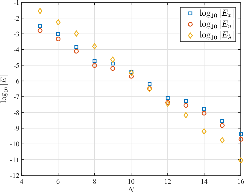
Figure 1 plots the logarithm of the sup-norm error in the state, control, and costate as a function of the number of collocation points. Since these plots are nearly linear, the error behaves like c​10−α​Nc10^{-\alpha N} where α≈0.6\alpha\approx 0.6 for either the state or the control and α≈0.8\alpha\approx 0.8 for the costate. In Theorem 1, the dependence of the error on NN is somewhat complex due to the connection between η\eta and NN. As we increase NN, we can also increase η\eta when the solution is infinitely differentiable, however, the norm of the derivatives also enters into the error bound as in (26). Nonetheless, in cases where the solution derivatives can be bounded by cηc^{\eta} for some constant cc, it is possible to deduce an exponential decay rate for the error as observed in [12, Sect. 2].
Refer to caption
Fig. 1: The base 10 logarithm of the error in the sup-norm as a function of the number of collocation points.

8 Conclusions

A Radau collocation scheme is analyzed for an unconstrained control problem. For a problem with a smooth solution and a Hamiltonian which satisfies a strong convexity assumption at a local minimizer of the continuous problem, we show that the discrete approximation has a local minimizer in a neighborhood of the continuous solution, and as the number of collocation points increases, the distance in the sup-norm between the discrete solution and the continuous solution is O⁡(N2−η)O(N^{2-\eta}) when the continuous solution has η+1\eta+1 continuous derivatives, η≥3\eta\geq 3, and the number of collocation points NN is sufficiently large. A numerical example is given which exhibits an exponential convergence rate.

9 Appendix

Before stating property (P3) in the Introduction, we showed that 𝐃‡{\bf D}^{\ddagger} is an invertible matrix. In this section, we give an analytic formula for the inverse.

Proposition 8.

The inverse of 𝐃‡{\bf D}^{\ddagger} is given by

Di​j‡−1=ωN​Mj​(1)+∫1τiMj​(τ)​dτ,1≤i<N,  1≤j<N,Di​N‡−1=−ωN,1≤i≤N,DN​j‡−1=ωN​Mj​(1),1≤j<N,\begin{array}[]{llll}D^{{\ddagger}\;-1}_{ij}&=&\omega_{N}M_{j}(1)+\int_{1}^{\tau_{i}}M_{j}(\tau)d\tau,&1\leq i<N,\;\;1\leq j<N,\\[3.61371pt] D^{{\ddagger}\;-1}_{iN}&=&-\omega_{N},&1\leq i\leq N,\\[3.61371pt] D^{{\ddagger}\;-1}_{Nj}&=&\omega_{N}M_{j}(1),&1\leq j<N,\end{array}

where MjM_{j}, 1≤j<N1\leq j<N, is the Lagrange interpolating basis relative to the point set τ1\tau_{1}, …\ldots, τN−1\tau_{N-1}. That is,

Mj(τ)=∏i=1i≠jN−1τ−τiτj−τi,j=1,…,N−1.M_{j}(\tau)=\displaystyle\prod_{\begin{subarray}{c}i=1\\ i\neq j\end{subarray}}^{N-1}\frac{\tau-\tau_{i}}{\tau_{j}-\tau_{i}},\quad j=1,\ldots,N-1.
Proof.

The relation (11) holds for any polynomial pp of degree at most N−1N-1. Let 𝐩˙∈ℝN\dot{{\bf{p}}}\in\mathbb{R}^{N} denote the vector with ii-th component p˙​(τi)\dot{p}(\tau_{i}). In vector form, the system of equations (11) can be expressed 𝐃‡​𝐩={\bf D}^{\ddagger}{\bf p}= 𝐩˙−𝐞N​p​(1)/ωN\dot{\bf p}-{\bf{e}}_{N}p(1)/\omega_{N}. Multiply by 𝐃‡−1{\bf{D}}^{{\ddagger}\;-1} and exploit the identity 𝐃‡−1​𝐞N=−ωN​𝟏{\bf{D}}^{{\ddagger}\;-1}{\bf{e}}_{N}=-\omega_{N}{\bf{1}} of (57) to obtain

𝐃‡−1​𝐩˙=𝐩−𝟏​p​(1).{\bf D}^{{\ddagger}\;-1}\dot{{\bf{p}}}={\bf{p}}-{\bf{1}}p(1). (61)

Since p˙\dot{p} is a polynomial of degree at most N−2N-2, we can only specify the derivative of pp at N−1N-1 distinct points. Given any jj satisfying 1≤j<N1\leq j<N, let us insert in (61) a polynomial p∈𝒫N−1p\in{\cal{P}}_{N-1} satisfying

p˙​(τj)=1andp˙​(τi)=0​ for all ​i<N,i≠j.\dot{p}(\tau_{j})=1\quad\mbox{and}\quad\dot{p}(\tau_{i})=0\mbox{ for all }i<N,\;\;i\neq j.

A specific polynomial with this property is

p⁡(τ)=∫1τMj​(τ)​𝑑τ.p(\tau)=\int_{1}^{\tau}M_{j}(\tau)d\tau. (62)

Since pN=p⁡(1)=0p_{N}=p(1)=0, the last component of the right side of (61) vanishes to give the relation DN​j‡−1+DN​N‡−1​p˙​(1)=0D_{Nj}^{{\ddagger}\;-1}+D_{NN}^{{\ddagger}\;-1}\dot{p}(1)=0. In (57) we showed that all the elements in the last column of 𝐃‡−1{\bf{D}}^{{\ddagger}\;-1} are equal to −ωN-\omega_{N}, and by (62), p˙​(1)=Mj​(1)\dot{p}(1)=M_{j}(1). Hence, we obtain the relation

DN​j‡−1=−DN​N‡−1​p˙​(1)=ωN​p˙​(1)=ωN​Mj​(1),  1≤j<N.D_{Nj}^{{\ddagger}\;-1}=-D_{NN}^{{\ddagger}\;-1}\dot{p}(1)=\omega_{N}\dot{p}(1)=\omega_{N}M_{j}(1),\;\;1\leq j<N. (63)

Finally, let us consider Di​j‡−1D_{ij}^{{\ddagger}\;-1} for i<Ni<N and j<Nj<N. We combine the ii-th component of (61) for i<Ni<N with (62) to obtain

(𝐃‡−1​𝐩˙)i=∫1τiMj​(τ)​𝑑τ.({\bf D}^{{\ddagger}\;-1}\dot{{\bf{p}}})_{i}=\int_{1}^{\tau_{i}}M_{j}(\tau)d\tau. (64)

Recall that all components of 𝐩˙\dot{{\bf{p}}} vanish except for the jj-th, which is 1, and the NN-th, which is Mj​(1)M_{j}(1) by (62). Hence, (64) and the fact that the elements in the last column of 𝐃‡−1{\bf{D}}^{{\ddagger}\;-1} are all −ωN-\omega_{N} yield

Di​j‡−1=∫1τiMj​(τ)​𝑑τ−Di​N‡−1​Mj​(1)=ωN​Mj​(1)+∫1τiMj​(τ)​𝑑τD_{ij}^{{\ddagger}\;-1}=\int_{1}^{\tau_{i}}M_{j}(\tau)d\tau-D_{iN}^{{\ddagger}\;-1}M_{j}(1)=\omega_{N}M_{j}(1)+\int_{1}^{\tau_{i}}M_{j}(\tau)d\tau

This completes the proof. ∎

As noted in the Introduction, the elements in the last row of 𝐃1:N−1{\bf{D}}_{1:N}^{-1} are positive and sum to 2, and the last row of 𝐃1:N−1𝐖−1/2{\bf{D}}_{1:N}^{-1}{\bf{W}}^{-1/2} is positive and has Euclidean norm 2\sqrt{2}. Numerically, we observe that the absolute row sums for the first N−1N-1 rows of 𝐃1:N−1{\bf{D}}_{1:N}^{-1} are always less than 2, while the Euclidean norm of the first N−1N-1 rows of 𝐃1:N−1𝐖−1/2{\bf{D}}_{1:N}^{-1}{\bf{W}}^{-1/2} are always less than 2\sqrt{2}. Properties (P3) and (P4) are less tight in the sense that the bounds only hold as equalities asymptotically. Tables 1 and 2 show ‖𝐃‡−1‖∞\|{\bf{D}}^{{\ddagger}\;-1}\|_{\infty} and the maximum Euclidean norm of the rows of 𝐃‡−1𝐖−1/2{\bf{D}}^{{\ddagger}\;-1}{\bf{W}}^{-1/2} for an increasing sequence of dimensions.

NN 25 50 75 100 125 150
norm 1.995376 1.998844 1.999486 1.999711 1.999815 1.999871
NN 175 200 225 250 275 300
norm 1.999906 1.999928 1.999943 1.999954 1.999962 1.999968
Table 1: ‖𝐃‡−1‖∞\|{\bf D}^{{\ddagger}\;-1}\|_{\infty}
NN 25 50 75 100 125 150
norm 1.412209 1.413691 1.413982 1.414083 1.414130 1.414156
NN 175 200 225 250 275 300
norm 1.414171 1.414181 1.414188 1.414193 1.414196 1.414199
Table 2: Maximum Euclidean norm for the rows of [𝐖1/2​𝐃‡]−1[{\bf{W}}^{1/2}{\bf D}^{\ddagger}]^{-1}

References

  • [1] C. L. Darby, W. W. Hager, and A. V. Rao, Direct trajectory optimization using a variable low-order adaptive pseudospectral method, AIAA Journal of Spacecraft and Rockets, 48 (2011), pp. 433–445.
  • [2]  , An hp-adaptive pseudospectral method for solving optimal control problems, Optim. Control Appl. Meth., 32 (2011), pp. 476–502.
  • [3] A. L. Dontchev and W. W. Hager, Lipschitzian stability in nonlinear control and optimization, SIAM J. Control Optim., 31 (1993), pp. 569–603.
  • [4]  , The Euler approximation in state constrained optimal control, Math. Comp., 70 (2001), pp. 173–203.
  • [5] A. L. Dontchev, W. W. Hager, and K. Malanowski, Error bounds for Euler approximation of a state and control constrained optimal control problem, Numer. Funct. Anal. Optim., 21 (2000), pp. 653–682.
  • [6] A. L. Dontchev, W. W. Hager, and V. M. Veliov, Second-order Runge-Kutta approximations in constrained optimal control, SIAM J. Numer. Anal., 38 (2000), pp. 202–226.
  • [7] G. Elnagar, M. Kazemi, and M. Razzaghi, The pseudospectral Legendre method for discretizing optimal control problems, IEEE Trans. Automat. Control, 40 (1995), pp. 1793–1796.
  • [8] G. N. Elnagar and M. A. Kazemi, Pseudospectral Chebyshev optimal control of constrained nonlinear dynamical systems, Comput. Optim. Appl., 11 (1998), pp. 195–217.
  • [9] F. Fahroo and I. M. Ross, Costate estimation by a Legendre pseudospectral method, J. Guid. Control Dyn., 24 (2001), pp. 270–277.
  • [10]  , Direct trajectory optimization by a Chebyshev pseudospectral method, J. Guid. Control Dyn., 25 (2002), pp. 160–166.
  • [11] D. Garg, M. A. Patterson, C. L. Darby, C. Françolin, G. T. Huntington, W. W. Hager, and A. V. Rao, Direct trajectory optimization and costate estimation of finite-horizon and infinite-horizon optimal control problems using a Radau pseudospectral method, Comput. Optim. Appl., 49 (2011), pp. 335–358.
  • [12] D. Garg, M. A. Patterson, W. W. Hager, A. V. Rao, D. A. Benson, and G. T. Huntington, A unified framework for the numerical solution of optimal control problems using pseudospectral methods, Automatica, 46 (2010), pp. 1843–1851.
  • [13] Q. Gong, I. M. Ross, W. Kang, and F. Fahroo, Connections between the covector mapping theorem and convergence of pseudospectral methods for optimal control, Comput. Optim. Appl., 41 (2008), pp. 307–335.
  • [14] W. W. Hager, Runge-Kutta methods in optimal control and the transformed adjoint system, Numer. Math., 87 (2000), pp. 247–282.
  • [15]  , Numerical analysis in optimal control, in International Series of Numerical Mathematics, K.-H. Hoffmann, I. Lasiecka, G. Leugering, J. Sprekels, and F. Tröltzsch, eds., vol. 139, Basel/Switzerland, 2001, Birkhauser Verlag, pp. 83–93.
  • [16] W. W. Hager, H. Hou, and A. V. Rao, Convergence rate for a Gauss collocation method applied to unconstrained optimal control, J. Optim. Theory Appl., submitted (2015, arxiv.org/abs/1507.08263).
  • [17]  , Lebesgue constants arising in a class of collocation methods, IMA J. Numer. Anal., submitted (2015, arxiv.org/abs/1507.08316).
  • [18] R. A. Horn and C. R. Johnson, Matrix Analysis, Cambridge University Press, Cambridge, 2013.
  • [19] S. Kameswaran and L. T. Biegler, Convergence rates for direct transcription of optimal control problems using collocation at radau points, Comput. Optim. Appl., 41 (2008), pp. 81–126.
  • [20] F. Liu, W. W. Hager, and A. V. Rao, Mesh refinement for optimal control using nonsmoothness detection and mesh size reduction, J. Franklin Inst., (2015, doi:10.1016/j.jfranklin.2015.05.028).
  • [21] J. Nocedal and S. J. Wright, Numerical Optimization, Springer, New York, 2nd ed., 2006.
  • [22] M. A. Patterson, W. W. Hager, and A. V. Rao, A p​hph mesh refinement method for optimal control, Optim. Control Appl. Meth., 36 (2015), pp. 398–421.
  • [23] G. W. Reddien, Collocation at Gauss points as a discretization in optimal control, SIAM J. Control Optim., 17 (1979), pp. 298–306.
  • [24] L. N. Trefethen, Approximation Theory and Approximation Practice, SIAM Publications, Philadelphia, 2013.
  • [25] P. Vértesi, On Lagrange interpolation, Period. Math. Hungar., 12 (1981), pp. 103–112.
  • [26] P. Williams, Jacobi pseudospectral method for solving optimal control problems, J. Guid. Control Dyn., 27 (2004), pp. 293–297.