It is a well known fact that our universe is expanding at an accelerated rate. There are many observational evidence for this [1][2][3][4][5]. One of the simplest candidates to describe the mysterious dark energy causing the acceleration is the cosmological constant $\Lambda$ introduced by Einstein to General Relativity to describe a static universe. The space-time with a positive cosmological constant is known as the de-Sitter space-time. Hence, our universe may be described by de Sitter geometry. There are several reasons to study de Sitter spaces. In high energy physics, there is a holographic duality relating quantum gravity on the de Sitter space to conformal field theory on a sphere of one dimension lower [6] [7] known as dS/CFT correspondence. Examples along those lines include, Kerr-de Sitter space-time in various dimensions studied by Dehghani [8] and holographic description of the three dimensional Kerr-de Sitter space with gravitational Chern-Simons term studied by Park [9]. One other reason for de Sitter space-times to gain lot of attention is the need to understand it in from the point of string theory. String theory is one of the popular candidates for a theory of quantum gravity. Hence, a fully satisfactory de Sitter solution to string theory has to be found. Towards this goal, classical solutions in Type IIB string theory have been studied by Dasguptha et.al [10]. Another work studying classical de Sitter solutions in string theory has been published by Danielsson et.al. [11].

Usually, a black hole is a space-time with a horizon and a singularity covered by the horizon. Contrary to this notion, there are black holes where there is a horizon but without a singularity at $r=0$. Such black holes are called “regular” black holes. The first regular black hole was constructed by Bardeen [12] [13] and interpreted as a magnetic monopole by Ay$\acute{o}$n-Beato and Garc$\acute{i}$a [14]. There are several other regular black hole solutions proposed by Ay$\acute{o}$n-Beato and Garc$\acute{i}$a [15][16][17][18]. In this paper, we are interested in studying one of the most interesting regular black holes proposed by Ay$\acute{o}$n-Beato and Garc$\acute{i}$a [15] and inteprited by Bronnikov [19]. This black hole is static, spherically symmetric and is described by two parameters, mass $M$ and magnetic charge $Q$. For $\frac{r}{M}>>1$ and for small $\frac{|Q|}{M}$, such black holes have similar properties as the well known Reissner-Nordstrom solution. This family of black hole solutions are referred to as ABGB black holes. Here we study the ABGB black hole in a de Sitter universe presented by Matyjasek et.al [20]. Since the current universe may be a one with a positive cosmological constant, it is important to understand regular black hole embedded in a de Sitter universe.

When a black hole is externally perturbed, the response can be described by three stages. The initial stage entirely depend on the initial data of the external perturbation. The intermediate stage correspond to damped oscillations with incomplete set of complex frequencies. These modes are called quasi-normal modes (QNM) and depend only on the macroscopic properties of the black hole such as the mass, spin and the charge. Measuring QNM frequencies using current gravitational wave detectors such as LISA, VIRGO and LIGO give a direct approach to detect black holes [21]. Other than for experimental reasons, there are also several theoretical aspects of black holes which are studied by using QNM frequencies. Due to the famous AdS/CFT correspondence, many works have been devoted to study QNM’s of black holes in anti-de Sitter space [22][23]. Black hole quantum spectrum via QNM were presented by Corda in [24]: the black hole model used by Corda is somewhat similar to the semi-classical Bohr’s model for the hydrogen atom. Another reason to create interest on QNM’s was the conjecture by Hod [25] relating quantum properties of black holes and asymptotic values of frequencies of QNM’s. There are many works devoted to compute asymptotic QNM frequencies due to this reason. Some recent work have addressed relation between QNM’s and hidden conformal symmetry of wave equations on the black hole back ground [26] [27]. Other than black holes, naked singularities also have been studied from the QNM point of view [28]. An excellent review on QNM’s is written by Konoplya and Zhidenko [29]. Given all the above, it is worthwhile to study QNM’s of regular black holes with nonlinear sources.

The paper is organized as follows: in section 2 an introduction to the regular-de Sitter black hole is given. In section 3 the scalar field perturbation is introduced. In section 4, the WKB approach to compute QNM are introduced. Massless scalar perturbation with QNM frequencies are presented in section 5. In section 6, analysis of $l=0$ mode of the massless scalar field is presented. In section 7, unstable null geodesics approach is used to compute QNM frequencies. In section 8, P$\ddot{o}$schl-Teller method to compute QNM frequencies are presented. In section 9 the conclusion is given.

In this section we will present the basic characteristics of a regular black hole with a positive cosmological constant derived by Matyjasek et.al [20]. The action from which it was derived is,

$$S=\frac{1}{16\pi G}\int\sqrt{-g}\left[(R-2\Lambda)-\mathcal{L}(F)\right]$$

(1)

Here $R$ is the scalar curvature and $\Lambda$ is the positive cosmological constant. $\mathcal{L(F)}$ is the Lagrangian for non-electrodynamics component given by,

$$\mathcal{L}(F)=F\left[1-tanh^{2}\left(\alpha\sqrt[4]{\frac{Q^{2}F}{2}}\right)\right]$$

(2)

Here $\alpha=\frac{|Q|}{2M}$ and $F=F_{\mu\nu}F^{\mu\nu}$ with $F_{\mu\nu}=\bigtriangledown_{\mu}A_{\nu}-\bigtriangledown_{\nu}A_{\mu}$. The only component of $F_{\mu\nu}$ which is non-zero for this solution is $F_{23}=F_{\theta\phi}$ given by,

$$F_{23}=Qsin\theta$$

(3)

Here, $Q$ is the magnetic charge. Hence,

$$F=\frac{2Q^{2}}{r^{4}}$$

(4)

Static spherically solutions for the action in eq.$(\ref{action})$ with the given magnetic field was derived in [20] to be,

$$ds^{2}=-f(r)dt^{2}+\frac{dr^{2}}{f(r)}+r^{2}d\Omega^{2}$$

(5)

where,

$$f(r)=1-\frac{2M}{r}\left(1-tanh\left(\frac{Q^{2}}{2Mr}\right)\right)-\frac{\Lambda r^{2}}{3}$$

(6)

This particular solution was named Ay$\acute{o}$n-Beato-Garc$\acute{i}$a-Bronnikov-de Sitter (ABGB-dS) solution.

The function $f(r)$ is finite at $r=0$. $f(r)$ can have at most three distinct roots leading to three horizons: $r_{c}$ is the cosmological horizon, $r_{b}$ is the event horizon and $r_{i}$ is the inner horizon. The region considered for the perturbations will be between $r_{b}$ and $r_{c}$. $f(r)$ also can have degenerate horizons: when $r_{i}=r_{b}$ they are referred to as cold black holes and when $r_{b}=r_{c}$, they are considered as charged Nariai black holes [30][31].

When $Q=0$, the metric yeilds the Schwarzschild-de Sitter black hole and when $\Lambda=0$, one obtain the ABGB black hole. Function $f(r)$ can be expanded for small $Q$ and for large $r$ as,

$$f(r)\approx 1-\frac{2M}{r}+\frac{Q^{2}}{r^{2}}-\frac{\Lambda r^{2}}{3}-\frac{Q^{6}}{12M^{2}r^{4}}+...$$

(7)

Hence, it is clear that for large $r$ and for small $Q$, the line-element resembles the well known Reissner-Nordstrom-de Sitter black hole (RNdS) with the line element eq.$(\ref{metric})$ with the function $f(r)$,

$$f(r)_{RNdS}=1-\frac{2M}{r}+\frac{Q^{2}}{r^{2}}-\frac{\Lambda r^{2}}{3}$$

(8)

The horizon structure of the ABGB-de Sitter black hole has been analyzed thoroughly in [20]. The regularized stress-energy tensor of the scalar, spinor and vector fields inside the degenerate ABGB-de Sitter black hole solution were studied by Matyjasek et.al [30].

Having introduced the geometry of the black hole space-time, in this section we will present perturbations by a minimally coupled scalar field around this geometry. The equations of motion for such a field is given by the Klein-Gordon equation,

$$(\bigtriangledown^{2}-\mu^{2})\eta=0$$

(9)

The scalar field $\phi$ can be decomposed into its partial modes as

$$\eta(r,\theta,\phi,t)=\sum_{l,m}e^{-i\omega t}Y_{l,m}(\theta,\phi)\frac{R(r)}{r}$$

(10)

Here, $Y_{l,m}(\theta,\phi)$ are spherical harmonics, and, $l$ and $m$ are the angular and the magnetic quantum numbers. $\omega$ is the frequency of the oscillations of the field. With the above decomposition, the radial component of the Klein-Gordon equation can be simplified to be,

$$\frac{d^{2}R(r_{*})}{dr_{*}^{2}}+\left(\omega^{2}-V_{scalar}(r_{*})\right)R(r_{*})=0$$

(11)

Here $r_{*}$ is the tortoise coordinates which is given by,

$$dr_{*}=\frac{dr}{f(r)}$$

(12)

and $V_{scalar}$ is given by,

$$V_{scalar}(r)=f(r)\left(\frac{l(l+1)}{r^{2}}+\frac{f^{\prime}(r)}{r}+\mu^{2}\right)$$

(13)

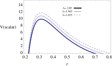
The effective potential approaches zero at $r=r_{b}$ ad $r=r_{c}$. It has a peak in between as demonstrated in Fig.$(\ref{potmass})$.

To get approximations for $r_{*}$, one can expand $f(r)$ around $r=r_{b,c}$ in a Taylor series as,

$$f(r)\approx f^{\prime}(r_{b,c})(r-r_{b,c})$$

(14)

Since $f^{\prime}(r_{c})<0$, $r_{*}$ can be derived to be,

$$r_{*}\approx-\frac{1}{|f^{\prime}(r_{c})|}Log(r_{c}-r)$$

(15)

Hence, when $r\rightarrow r_{c}$, $r_{*}\rightarrow\infty$. Similarly, since $f^{\prime}(r_{b})>0$, $r_{*}$ can be derived to be,

$$r_{*}\approx\frac{1}{|f^{\prime}(r_{b})|}Log(r-r_{b})$$

(16)

Hence, when $r\rightarrow r_{b}$, $r_{*}\rightarrow-\infty$. Hence the effective potential $V_{scalar}\rightarrow 0$ when $r_{*}\rightarrow\pm\infty$.

QNM for a black hole perturbed by a scalar field is given by the solutions of the wave eq.$(\ref{wave})$. To find the QNM solutions one has to impose boundary conditions; it is purely ingoing field at the even horizon $r_{b}$ and purely outgoing fields at the cosmological horizon $r_{c}$. The frequencies corresponding to the QNM are given by $\omega=\omega_{R}+i\omega_{I}$; here $\omega_{R}$ is the oscillating component and $\omega_{I}$ is the damping component of the frequency. QNM for eq.$(\ref{wave})$ with the above mentioned boundary conditions can be represented as,

$$R(r_{*})\rightarrow exp(i\omega r_{*});\hskip 28.45274ptr_{*}\rightarrow-\infty(r\rightarrow r_{b})$$

(17)

$$R(r_{*})\rightarrow exp(-i\omega r_{*});\hskip 28.45274ptr_{*}\rightarrow+\infty(r\rightarrow r_{c})$$

(18)

Since the effective potential has a peak and has the form of a potential barrier, to find the QNM frequencies, one can use the WKB approach. WKB approach to find QNM frequencies of black holes was first developed by Iyer and Will for third order [32]; it was later extended to sixth order by Konoplya [33]. The sixth order WKB approximation is employed to find QNM frequencies in several papers including, [13] [34] [35].

In the sixth order WKB approach, QNM frequencies are given by the expression,

$$\omega^{2}=-i\sqrt{-2V^{\prime\prime}(r_{max})}\left(\sum^{6}_{i=2}\Gamma_{i}+n+\frac{1}{2}\right)+V(r_{max})$$

(19)

Here, $r_{max}$ is where $V(r)$ reach a maximum and $V^{\prime\prime}(r)$ is the second derivative of the potential. Expressions for $\Gamma_{i}$ can be found in [33].

First, we will focus on the massless scalar field perturbations where $\mu=0$. In this case, the effective potential $V_{scalar}$ depend on the parameters, $M,Q,l$ and $\Lambda$. In Fig.$(\ref{potmass})$, the potential is plotted by varying $M$. When the mass $M$ increases, the height of the potential decreases. In Fig.$(\ref{potcharge})$, $V_{scalar}$ is plotted by increasing the charge $Q$. When $Q$ is increased, the height of the potential increased. When the cosmological constant $\Lambda$ is increased, the height of the potential decreases as given in Fig.$(\ref{potlambda})$. In Fig$(\ref{potl})$, the potential is plotted by varying $l$ where $l$ is positive. When $l$ increases, the potential increases. In Fig$(\ref{pot2})$, the potential is plotted for $l=1$ and $l=0$. It is interesting to notice that the potential for $l=0$ has a local minimum between the two horizons, $r_{h}$ and $r_{c}$ which is different from the behavior of the potential for other values of $l$.

As given in Fig.$(\ref{pot2})$, potential for $l=0$ modes is rather different from all other potential with $l>0$. The difference is attributed to the fact that the potential is negative in a range between the black hole horizon and the cosmological horizon. In fact, similar behavior persists for $l=0$ potential for both Schwarzschild-de Sitter black hole and the Riessner-Nordstrom-de Sitter black hole as shown in Fig$(\ref{potboth2})$.

WKB approximation that was used in section(5.1) to compute the QNM frequencies of $l>0$ modes are not suitable to compute the frequencies of $l=0$ modes since there is an extra local minimum of the potential. Hence we will avoid computing the QNM frequencies for this case. Instead, we would be interested in understanding if the black hole is stable under the $l=0$ mode perturbations. In fact, when the potential is negative in some region, it is possible to have growing QNM modes leading to instability of the system under such perturbations. However, it turns out that this is not the case for all cases with negative potentials as discussed in [36]. What we would present here is to the fact that the field of $l=0$ mode in fact settle in to a constant value at late times. Since one of the reasons to study QNM frequencies is to understand the stability of the black hole under such perturbations, such a study is appropriate. If one needs to compute the QNM frequencies, and see how the field evolves, then a time-domain integration method used by Gundlach et.al. in [38] can be used. Instead, we will present an analytical observation of how the field behaves at late time.

$l=0$ mode does approach a constant value for the Schwarzschild-de Sitter black hole as presented by Brady et.al [37]. We will use similar approach to show the behavior of the field around the regular-de Sitter black hole.

Here, we will study the scattering of the field between $r_{b}$ and $r_{c}$ for $l=0$ mode. First we will introduce null coordinates $u$ and $v$ as,

$$u=t-r_{*};\hskip 28.45274ptv=t+r_{*}$$

(21)

Here, $r_{*}$ is the tortoise coordinate introduced in eq.$(\ref{tor})$. Then, the line element in eq.$(\ref{metric})$ simplifies to

$$ds^{2}=-f(r)dudv+r^{2}d\Omega^{2}$$

(22)

According to the null coordinates, the future cosmological horizon, $r=r_{c}$ is located at $v=\infty$ and the future black hole horizon, $r_{b}$ is located at $u=\infty$. Now, in terms of the null coordinates, the scalar wave equation $\bigtriangledown^{2}\eta=0$ for a massless scalar field simplifies to,

$$\frac{\partial^{2}\Psi(u,v)}{\partial u\partial v}=-\frac{1}{4}V_{l=0}(r)\Psi(u,v)$$

(23)

where,

$$\eta(u,v,\theta,\phi)=\sum_{l,m}Y_{l,m}(\theta,\phi)\frac{\Psi(u,v)}{r}$$

(24)

and

$$V_{l=0}=\frac{f(r)f^{\prime}(r)}{r}$$

(25)

Notice that for $l=0$, the potential simplifies.

When $l=0$, the solution to the eq.$(\ref{wave3})$ can be expressed as a series depending on two arbitrary functions $G(u)$ and $H(v)$ as [37][38],

$$\Psi=A\left(G(u)+H(v)\right)+\sum_{p=0}^{\infty}B_{p}(r)[G^{(-p-1)}(u)+(-1)^{p+1}H(v)^{(-p-1)}]$$

(26)

Here, the negative super indices on $G$ and $H$ refer to integration with respect to $u$ and $v$ respectively: for example, $G^{-1}(u)=\int G(u)du$. The coefficient $A$ can be set equal to $1$ without loss of generality.

When eq.$(\ref{expansion})$ is substituted to eq.$(\ref{wave3})$, one can compare the coefficients to come up with a recurrence relations for $B_{p}(r)$ as,

$$B_{p+1}^{\prime}=\frac{f^{\prime}}{2r}\left(-B_{p}+rB_{p}^{\prime}\right)+\frac{f}{2}B_{p}^{\prime\prime}$$

(27)

Here,

$$B_{0}=-\int\frac{f^{\prime}}{2r}dr$$

(28)

To facilitate the computation, we will assume the charge $Q$ is small and do an expansion for the function $f(r)$ for the regular de-Sitter black hole as,

$$f(r)\approx 1-\frac{2M}{r}+\frac{Q^{2}}{r^{2}}-\frac{Q^{6}}{12M^{2}r^{4}}$$

(29)

Note that the qualitative behavior of the black hole outside $r_{b}$ and inside $r_{c}$ are not much different in the expansion. Now, one can integrate eq.$(\ref{bnote})$ to obtain $B_{0}$ as,

$$B_{0}=\frac{Q^{6}}{30M^{2}r^{5}}-\frac{Q^{2}}{3r^{3}}+\frac{M}{2r^{2}}+\frac{r\Lambda}{3}$$

(30)

From the recurrence relation in eq.$(\ref{recur})$, $B_{1}$ can be obtained to be,

$$B_{1}=\sum_{n=3}^{11}\frac{a_{n}}{r^{n}}$$

(31)

where $a_{n}$ depends on $M,Q$ and $\Lambda$. Other $B_{p}$ values with $p>1$ also behaves similarly with higher powers of $\frac{1}{r}$ terms. For large $r$, $B_{p}$ will vanish except for $B_{0}$. This is one of the major difference compared to an asymptotically flat black hole where all $B_{p}$ values will vanish for large $r$.

Now, we consider an initial burst of radiation on $v=0$. The radiation is confined between $u=0$ and $u=u_{1}$ and is given by $\Psi(u,0)=G(u)$. Also, $\Psi(0,v)=0$. This is demonstrated in Fig.$(\ref{draw})$. We want to study the evolution of this field in the diamond shape region given in Fig.$(\ref{draw})$ by thick lines.

Following the work by Gundlach et.al [38] and Brady et.al. [37], the evolution of the initial burst can be broken into two parts: (i) the evolution of the burst $\Psi(u,0)=G(u)$ which is non-zero between $0<u<u_{1}$ and $\Psi(0,v)=0$. (ii) subsequent evolution in the region for $u\geq u_{1}$.

The black holes considered in this paper have unstable null geodesics. Cardoso et.al. [39], showed that in the eikonal limit ($l>>1$), QNM of a black hole can be determined by the parameters of null geodesics. An earlier work done along those lines is given by Mashhon [40]

An expansion method to compute QNM based on the link between the null geodesics and QNM freuencies has been applied to Kerr black hole in a paper by Dolan [41]. The method of null geodesics has been applied to study the near-extreme Kerr black hole by Hod [42] and black holes in anti-de Sitter space by Morgan et.al in [43].

The equation of motion for massless particles around a black hole is given by [44]

$$\dot{r}^{2}+V_{null}=E^{2}$$

(40)

with,

$$V_{null}=\left(\frac{L^{2}}{r^{2}}\right)f(r)$$

(41)

Here, $L$ is the angular momentum of the massless particle. For bot $r=r_{h}$ and $r=r_{c}$, $V_{null}=0$. In the Fig.$(\ref{potnull})$, $V_{null}$ is plotted for various values of the magnetic charge $Q$. One can observe that the height of the potential is higher for higher values of $Q$.

Now, when the effective potential for the massless scalar field $V_{scalar}$ in eq.(17) is studied, one can see that in the eikonal limit ($l\rightarrow\infty$),

$$V_{scalar}\approx\frac{f(r)l}{r^{2}}$$

(42)

Hence, one can conclude that the maximum of $V_{scalar}$ occurs at $r=r_{max}$ given by,

$$2f(r_{max})-r_{max}f^{\prime}(r_{max})=0$$

(43)

On the other hand, the maximum of $V_{null}$ occurs at $V_{null}^{\prime}=0$ leading to,

$$2f(r_{null})-r_{null}f^{\prime}(r_{null})=0$$

(44)

Hence the maximum of $V_{scalar}$ and the location of the maximum of the null geodesics coincides at $r_{max}=r_{null}$. $V_{null}(r)^{\prime}=0$ leads to the equation,

$$\frac{Q^{2}}{r^{5}}Sech^{2}\left(\frac{Q^{2}}{2Mr}\right)+\frac{2}{r^{4}}\left(-3M+r+3MTanh\left(\frac{Q^{2}}{2Mr}\right)\right)=0$$

(45)

Solutions to the above equation gives $r_{null}$ values. Since an analytical expression is not possible, we have calculated $r_{null}$ varying charge $Q$ numerically and plotted in Fig.$(\ref{rnull})$. One can observe that $r_{null}$ gets smaller as $Q$ increases.

According to [39] the QNM frequencies in the eikonal limit is given by,

$$\omega_{QNM}=\Omega_{a}l-i(n+\frac{1}{2})|\lambda_{Ly}|$$

(46)

Here, $l$ is the angular momentum of the perturbation and $n$ is the overtone number, and $\Omega_{a}$ is the coordinate angular velocity given as,

$$\Omega_{a}=\frac{\dot{\phi}}{\dot{t}}$$

(47)

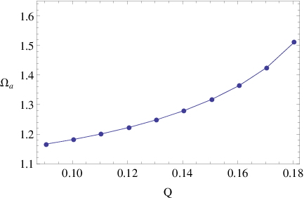
The parameter $\lambda_{Ly}$ appearing in eq.$(\ref{nullfre})$ is the Lyapunov exponent which is interpreted as the decay rate of the unstable circular null geodesics. The derivation of the above results is explained in Cardoso et.al[39]. For the ABGB-dS black hole, $\Omega_{a}$ and $\lambda_{Ly}$ are given as,

$$\Omega_{a}=\frac{\dot{\phi}(r_{null})}{\dot{t}(r_{null})}=\sqrt{\frac{f(r_{null})}{r_{null}^{2}}}$$

(48)

$$\lambda_{Ly}=\sqrt{\frac{-V_{null}^{\prime\prime}(r_{null})}{2\dot{t}(r_{null})^{2}}}=\sqrt{\frac{-V_{null}^{\prime\prime}(r_{null})r_{null}^{2}f(r_{null})}{2L^{2}}}$$

(49)

By using $\Omega_{a}$ and $\lambda_{Ly}$, the QNM frequencies are calculated and plotted in Fig.$(\ref{lya})$ and Fig.$(\ref{angular})$. When compared with $\omega$ values computed with WKB approach given in Fig$(\ref{omegacharge})$, one can conclude that they are similar in behavior.

First we like to discuss the extreme ABGB-dS black hole when $r_{b}=r_{c}$. For the black hole to be extreme, two conditions has to be satisfied:

$$f(r)=0;\hskip 28.45274ptf^{\prime}(r)=0$$

(50)

Due to the complex nature of the function $f(r)$, an exact value for $r_{b}$ for the extreme black hole is not possible. Let us name the value of $r_{b}$ at this special case as $\sigma$. It is clear that $f^{\prime\prime}(\sigma)<0$ due to the nature of the function $f(r)$. Such extreme black holes where $r_{b}=r_{c}$ are called Nariai black holes [31][45][46].

In the near extreme case, $r_{b}$ and $r_{c}$ are very close. Hence $f(r)$ can be expanded in a Taylor series as [30] as,

$$f(r)\approx\frac{f^{\prime\prime}(\sigma)}{2}(r-r_{b})(r-r_{c})$$

(51)

Hence the tortoise coordinate defined as $r_{*}=\int\frac{dr}{f(r)}$ can be integrated as,

$$r_{*}=\int\frac{dr}{f(r)}=\frac{2}{f^{\prime\prime}(\sigma)(r_{c}-r_{b})}log\left(\frac{r_{c}-r}{r-r_{b}}\right)$$

(52)

From the above derivation, it is clear that when $r\rightarrow r_{b}$, $r_{*}\rightarrow-\infty$ and $r\rightarrow r_{c}$, $r_{*}\rightarrow\infty$. From the relation in eq.$(\ref{newtr})$ can be solved for $r$ as,

$$r=\frac{r_{b}+r_{c}e^{\rho r_{*}}}{1+e^{\rho r_{*}}}$$

(53)

Here,

$$\rho=-\frac{f^{\prime\prime}(\sigma)}{2}(r_{c}-r_{b})$$

(54)

Bu substituting $r$ in eq.$(\ref{rvalue})$, the function $f(r)$ for the near extreme ABGB-de Sitter black hole can be written as,

$$f(r)=\frac{\xi}{4(Cosh(\frac{\rho r_{*}}{2}))^{2}}$$

(55)

Here,

$$\xi=-\frac{f^{\prime\prime}(\sigma)}{2}(r_{c}-r_{b})^{2}$$

(56)

Now the effective potential for the scalar field can be written as,

$$V_{eff}=\frac{V_{0}}{Cosh^{2}(\frac{\rho r_{*}}{2})}$$

(57)

where

$$V_{0}=\frac{\xi l(l+1)}{4\sigma^{2}}+\frac{\xi}{4}\mu^{2}$$

(58)

In deriving $V_{0}$, we have assumed $r\approx\sigma$. Also since $f(r)^{\prime}\approx 0$, only the first term in the potential dominates. With the new definition of the potential, the wave equation for the scalar field perturbations simplifies to,

$$\frac{d^{2}\Omega(r_{*})}{dr_{*}^{2}}+\left(\omega^{2}-\frac{V_{0}}{Cosh^{2}(\frac{\rho r_{*}}{2})}\right)\Omega(r_{*})=0$$

(59)

$\frac{V_{0}}{Cosh^{2}(\frac{\rho r_{*}}{2})}$ is the well known P$\ddot{o}$schl-Teller potential and Ferrari and Mashhoon, in a well known paper [47] demonstrated that $\omega$ can be computed exactly as,

$$\omega=\sqrt{V_{0}-\frac{\rho^{2}}{16}}-i\frac{\rho}{2}(n+\frac{1}{2})$$

(60)

By observing the expression for $\omega$ given above, some hand waving arguments of the behavior of $\omega$ can be made. When $\mu$ is large, and $l$ is small, $V_{0}\approx\frac{\xi\mu^{2}}{4}$. Hence, $\omega_{R}\approx\frac{\sqrt{\xi}\mu}{2}+constant$ and $\omega_{R}$ will depend linearly on $\mu$. On the other hand, $\omega_{I}$ does not depend on $\mu$ for extreme black holes. When the spherical harmonic index $l$ is large, $V_{0}\approx\frac{\xi l^{2}}{4\sigma^{2}}$. Hence $\omega_{R}\approx\frac{\sqrt{\xi}l}{2\sigma}+constant$. Hence $\omega_{R}$ depends on $l$ linearly for large $l$ which is clear from Fig$(\ref{sphereal})$. For large $l$, $\omega_{I}$ is independent of $l$ and is clear from Fig$(\ref{spheima})$. For large $n$, $\omega_{I}$ becomes large and $\omega_{R}$ is independent of $n$. This behavior is represented in Fig.$(\ref{omegan})$.

Our main goal in this paper has been to study QNM and stability of a regular black hole in de Sitter universe under scalar perturbations. The regular black hole does not have a singularity at $r=0$. It has three horizons: cosmological horizon $r_{c}$, black hole event horizon $r_{b}$ and inner horizon $r_{i}$. The structure of the regular-de Sitter black hole is very similar to the Reissner-Nordstrom-de Sitter black hole.

We have employed sixth order WKB approximation to compute QNM frequencies. The parameters of the theory, the mass $M$, magnetic charge $Q$, cosmological constant $\Lambda$ and the spherical index $l$ and the mode number $n$ were changed to see how QNM frequencies depend on them. When $Q$ is increased, $\omega_{R}$ increases. On the other hand, when $Q$ is increased, $\omega_{I}$ increases to a maximum and then decreases for large $Q$. Hence, there is a particular value of $Q$ where the black hole have the most stability. We have observed the behavior of the quality factor for the black hole as a function of the charge $Q$. It is noticed that the larger the charge, larger the quality factor is.

Next, we have plotted $\omega$ as a factor of the black hole $r_{b}$. When $r_{b}$ increases, $\omega_{R}$ decreases and $\omega_{I}$ increases to a maximum and then decreases. Hence there is a particular size of the black hole where the stability is maximized. We have also computed the Hawking temperature to observe the relation with $\omega_{I}$. The relation is not linear as in other black holes.

We have studied the behavior of $\omega$ with the cosmological constant $\Lambda$. When $\Lambda$ is increased, both $\omega_{R}$ and $\omega_{I}$ decreases. Hence, a smaller $\Lambda$ is favored for a stable black hole. The behavior of $\omega$ with respect to $l$, the spherical harmonic index is similar to the behavior of other black holes. $\omega_{R}$ has a linear relation with $l$ and $\omega_{I}$ is independent of $l$ for large $l$. We have also plotted $\omega$ vs $n$, the mode number. Here, $\omega_{R}$ decreases with $n$ and $\omega_{I}$ increases linearly with $n$.

The $l=0$ mode for the massless field presents a potential with a negative region between $r_{b}$ and $r_{c}$. WKB approach cannot be used to compute QNM frequencies in such a case since there is an additional local minimum in the potential. Instead, we did an analytical study to show that an initial burst of radiation will settle into a constant value at late times. Such behavior have been observed for the $l=0$ mode for the d Schwarzschild-de Sitter black holes.

In addition to the WKB approach, we have used the unstable null geodesics approach to compute $\omega$ for massless scalar fields. First we observe that the radius of the unstable null geodesic $r_{null}$ decreases with $Q$. The coordinate angular velocity, which is proportional to $\omega_{R}$ increases with $Q$. The Lyapunov exponent which is proportional to $\omega_{I}$ does show similar behavior as was done using WKB approach.

Finally, we have demonstrated that for the near-extremal black hole with $r_{b}\approx r_{c}$ the scalar field equation will have the P$\ddot{o}$schl-Teller potential; one can get exact expressions for he QNM frequencies for this observation. Most of the observation we did with WKB approach, tally with the exact expressions obtained via this method.

As future work, it may be interesting to compute QNM frequencies and study stability of the massive fields. We did not use WKB approach to compute QNM frequencies of this case since there may be extra local minima for the potential. One may use continued fraction method used by Konoplya and Zhidenko [48] to compute massive QNM for the Schwarzschild black hole.

Acknowledgments: The author wish to thank R. A. Konoplya for providing the Mathematica file for the WKB approximation.

References

- [1] S. Perlmutter et. al., Measurements of and from 42 high-redshift supernovae, Astrophys. J. 517 565 (1999)
- [2] A.G. Riess et. al., Observational evidence from supernovae for an accelerating universe and a cosmological constant, Astron. J. 116 1009 (1998); BVRI Light Curves for 22 Type Ia Supernovae, Astron. J. 117 707(1999)
- [3] D. N. Spergel et.al. (WMAP Collaboration), Wilkinson Microwave Anisotropy Probe (WMAP) three year results: implications for cosmology, Astrophys. J. Suppl. 170 377 (2007)
- [4] M. Tegmark et.al. (SDSS Collaboration) Cosmological parameters from SDSS and WMAP , Phys. Rev. D 69 103501 (2004)
- [5] U. Seljak et.al., Cosmological parameter analysis including SDSS Ly forest and galaxy bias: constraints on the primordial spectrum of fluctuations, neutrino mass, and dark energy, Phys. Rev. D 71 103515 (2005)
- [6] E. Witten, Quantum gravity in de Sitter space: hep-th/0106109
- [7] A. Strominger, The dS/CFT correspondence, hep-th/0106113
- [8] M. H. Dehghani, Kerr-de Sitter spacetimes in various dimensions and dS/CFT correspondence, Phys. Rev. D 65 104003 (2002)
- [9] M. Park, Holography in Kerr-de Sitter space with a gravitational Chern-Simons term, Class. Quant. Grav. 25 135003 (2008)
- [10] K. Dasguptha, R. Gwyn, E. McDonough, M. Mia, & R. Tatar, de Sitter vacua in Type II B string theory: classical solutions and quantum corrections, JHEP 054:1407 (2014)
- [11] U. H. Danielsson, S. S. Haque, G. Shiu, & T. van Riet, Towards classical de Sitter solutions in string theory, JHEP 0909:114 (2009)
- [12] J. Bardeen, Proceedings of GR5, Tiflis, U.S.S.R. page 174 (1968)
- [13] S. Fernando & J. Correa, Quasi-normal modes of the Bardeen black hole: scalar perturbations, Phys. Rev. D 86 64039 (2012)
- [14] E. Ayón-Beato and A. García, The Bardeen model as a nonlinear magnetic monopole , Phys. Lett B 493 149 (2000)
- [15] E. Ayón-Beato and A. García, New regular black hole solution from non-linear electrodynamics, Phys. Lett B 464 25 (1999)
- [16] E. Ayón-Beato and A. García, Non singular charged black hole solution for non-linear source, Gen. Rel. Grav. 31 629 (1999)
- [17] E. Ayón-Beato and A. García, Four parametric regular black hoe solution, Gen. Rel. Grav. 37 635 (2005)
- [18] E. Ayón-Beato and A. García, Regular black hole in general relativity coupled to nonlinear electrodynamics, Phys. Rev. Lett. 80 5056 (1998)
- [19] K. A. Bronnikov, Regular magnetic black holes and monopoles from nonlinear electrodynamics, Phys. Rev. D 63 044005 (2001)
- [20] J. Matyjasek, D. Tryniecki, & M. Klimek, Regular black holes in an asymptotically de Sitter universe, Mod. Phys. Lett. A 23 3377 (2009)
- [21] V. Ferrari & L. Gualtieri, Quasi-normal modes and gravitational wave astronomy, Gen. Rel. Grav. 40 945 (2008)
- [22] V. Cardoso & G. Khanna, Black holes in anti-de Sitter: quasinormal modes, tails and tales of flat spacetime, Phys. Rev. D91 024031 (2015)
- [23] G.T. Horowitz & V. E. Hubeny, Quasinormal modes of AdS black holes and the approach to thermal equilbrium, Phys. Rev. D62 024027 (2000)
- [24] C. Corda, Black hole spectrum, Eur. Phys. Jour C 73 2665 (2013)
- [25] S. Hod, Bohr’s correspondence principle and the area spectrum of quantum black holes, Phys. Rev. Lett. 81 4293 (1998)
- [26] B. Chen, J. Zhang, J. Zhang, Quasinomrmal modes and hidden conformal symmetry of warped black hole, Phys. Rev. 84 124039 (2011)
- [27] Y. Kim, Y. S. Myung and Y. Park, Quasinormal modes and hidden conformal symmetry in the Reissner-Nordstrom black hole, Eur. Phys. Jour. C 73 2440 (2013)
- [28] C. Chirenti, A. Saa and J. Skakala, Quasinormal modes for the scattering on a naked Reissner-Nordstrom singularity, Phys. Rev. D 86 124008 (2012)
- [29] R. A. Konoplya and A. Zhidenko, Quasinormal modes of black holes: from astrophysics to string theory, Rev. Mod. Phys. 83 793 (2011)
- [30] J. Matyjasek, P. Saurski & D. Tryniecki, Inside the degenerate horizons of regular black holes, Phys. Rev. D 87 124025 (2013)
- [31] S. Fernando, Cold, ultracold and Nariai black holes with quintessence, Gen. Rel. Grav. 45 2053 (2013)
- [32] S. Iyer & C.M. Will, Black-hole normal modes: A WKB approach. I. Foundations and application of a higher-order WKB analysis of potential-barrier scattering, Phys. Rev. D 35 3621(1987)
- [33] R. A. Konoplya, Quasinormal behavior of the D-dimensional Schwarzschild black hole and higher order WKB approach, Phys. Rev. D68 024018 (2003)
- [34] R. Konoplya, Quasinormal modes of the charged black hole in Gauss-Bonnet gravity, Phys. Rev. D 71 024038 (2005)
- [35] S. Fernando & T. Clark, Black holes in massive gravity: quasinormal modes of scalar perturbations, Gen. Rel. Grav. 46 1834 (2014)
- [36] K. A. Bronnokov, R. A. Konoplya & A. Zhidenko, Instabilities of wormholes and regular black holes supported by phantom scalar field, Phys. Rev. D 86 024028 (2012)
- [37] P. R. Brady, C. M. Chambers, W. Krivan, & P. Laguna, Telling tails in the presence of a cosmological constant, Phys. Rev. D 55 7538 (1997)
- [38] C. Gundlach, R. H. Price, & J. Pullin, Late-time behavior of stellar collapse and explosions: I Linearized perturbations, Phys. Rev. D 49 883 (1994)
- [39] V. Cardoso, A.S. Miranda, E. Berti, H. Witeck & V.T. Zanchin, Geodesic stability, Lyapunov exponents and quasinormal modes, Phys.Rev. D79 ( 2009) 064016
- [40] B. Mashhoon, Stability of charged rotating black holes in the eikonal approximation, Phys. Rev. D31 (1985) 290
- [41] S. R. Dolan, The quasinormal mode spectrum of a Kerr black hole in the eikonal limit, Phys. Rev. D82 (2010) 104003
- [42] S. Hod, Black-hole quasinormal resonances: wave analysis versus a geometrical-optics approximation, Phys. Rev. D80 (2009) 064004
- [43] J. Morgan, V. Cardoso, A. S. Miranda, C. Molina and V. T. Zanchin, Quasinormal modes of black holes in anti-de Sitter space: a numerical study of the eikonal limit, Phys. Rev. D80 (2009) 024024
- [44] S. Fernando, Null geodesics of charged black holes in string theory, Phys. Rev. D85, 02403 (2012)
- [45] S. Fernando, Nariai black holes with quintessence, Mod. Phys. Lett. A 28 13550189 (2013)
- [46] S. Fernando, Born-Infeld-de Sitter gravity: cold, ultracold and Nariai black holes, Int. Jour. Mod. Phys. D 22 1350080 (2013)
- [47] V. Ferrari & B. Mashhoon, New approach to the quasinormal modes of a black hole, Phys. Rev. D30 295 ( 1984)
- [48] R. A. Konoplya and A. V. Zhidenko, Decay of massive scalar field in a Schwarzschild background, Phys. Lett. B 609 377(2005)