Production cross section estimates for strongly-interacting
Electroweak Symmetry Breaking Sector resonances
at particle colliders
Abstract
We are exploring a generic strongly-interacting Electroweak Symmetry Breaking Sector (EWSBS) with the low-energy effectie field theory for the four experimentally known particles (, , ) and its dispersion-relation based unitary extension. In this contribution we provide simple estimates for the production cross section of pairs of the EWSBS bosons and their resonances at proton-proton colliders as well as in a future (or potentially a ) collider with a typical few-TeV energy. We examine the simplest production mechanisms, tree-level production through a (dominant when quantum numbers allow) and the simple effective boson approximation (in which the electroweak bosons are considered as collinear partons of the colliding fermions). We exemplify with custodial isovector and isotensor resonances at 2 TeV, the energy currently being discussed because of a slight excess in the ATLAS 2-jet data. We find it hard, though not unthinkable, to ascribe this excess to one of these rescattering resonances. An isovector resonance could be produced at a rate smaller than, but close to earlier CMS exclusion bounds, depending on the parameters of the effective theory. The excess is then problematic and requires additional physics (such as an additional scalar resonance). The isotensor one (that would describe all charge combinations) has a smaller cross section.
1 Introduction
If physics beyond the SM exists, the lack of any manifestation in the few-hundred GeV region and the lightness of the new Higgs-like boson naturally suggest that this particle could be a quasi-Goldstone boson beyond the three needed for Electroweak Chiral Symmetry Breaking. This would call for enlarging the Standard Model (SM) symmetry group, leading perhaps to composite Higgs models.
Independently of this, the current spectrum in the 100 GeV region consists of the custodial-isospin triplet of and bosons together with the new Higgs boson . A general formulation of the Electroweak Symmetry Breaking Sector (EWSBS) in terms of effective field theory (in the non-linear realization of ) can be encoded, neglecting boson masses, in the seven-parameter next-to-leading order (NLO) Lagrangian density
| (1) | |||||
that we have described in detail in Refs. [1, 2]. (See also Refs. [3, 4, 5] and references therein for additional background.)
The Equivalence Theorem (ET) [6] relates the amplitudes of these Goldstone bosons (GBs) to those of the longitudinal components of the electroweak gauge bosons, and in the SM and can also be extended to effective field theories [7] with larger particle/interaction content.
The effective Lagrangian of Eq. (1) is useful in the 0.5–3 TeV region: for TeV the ET starts receiving large corrections, and for TeV the derivative expansion breaks down. It includes the newly found field coupled as an singlet in a custodially-invariant way, but we are not concerned with it in this work, that concentrates on production with non-vanishing custodial isospin. The reason for this focus is that the much commented ATLAS diboson excess [8], barring misidentification, is seen in all , and channels. A similar philosophy has been followed by the Barcelona group [9].
If new resonances beyond the SM appear in the spectrum, the pure (polynomial-like) momentum expansion fails before the scale as is well-known from hadron physics, where there are elastic pion-pion resonances below GeV. The useful tools are then dispersion relations, whose subtraction constants are fixed by the effective theory, so that elastic (or coupled-channel, in the chiral limit) unitarity is exactly enforced. In Appendix A.2 we quickly review the resulting Inverse Amplitude Method (IAM) [10, 11] that provides us with scattering amplitudes that are unitary, have the right analytic properties for complex Mandelstam variable , match perturbation theory based on the Lagrangian in Eq. (1) and are encoded in a very simple algebraic formula, without the need for tedious numerical solutions of involved integral equations. Resonances can then be generated as poles of the unitarized scattering amplitudes.
In this contribution we address the production cross section of exemplary resonances generated by the IAM. We examine two production mechanisms, the collision of two longitudinal bosons collinear with the beam particles (effective boson approximation) in Section 2 yielding an isotensor resonance, and the production of an isovector one by an intermediate gauge boson in Section 3.
As will be shown in Section 4, the intermediate- boson mechanism for the production of an isovector -like resonance is larger (since the isospin Clebsch–Gordan coefficients impede the data would be ascribed to misidentification or to a concurrent scalar resonance as noted in [12]). The computed cross section for the production of an isovector resonance (around 18 fb/TeV at 2 TeV) is just smaller than the related bounds provided by the CMS collaboration in Ref. [13] (about 20 fb/TeV there). We conclude that an ATLAS excess with the same data base could only marginally be generated by a resonance stemming purely from the EWSBS, though further more detailed studies appear necessary.
Explanations invoking strong coupling of the new physics to quarks and gluons have recently been proposed, but we do not address those.
2 Cross section from collinear s
2.1 Lepton-lepton collisions
We start and settle notation with the effective approximation [14] in collisions, that amounts to treating the as a collinear parton of the lepton pair or . Then one can write down collinear factorization formula for the process (with representing a pair of or ), as shown in Fig. 1, in terms of the parton-parton ( in this case) cross section.

The differential cross section for this production process as a function of the total center-of-mass energy may be written as [15]
| (2) |
where inside the integral is the cross section for the process with all the particles on-shell, is the center-of-mass energy of the initial, colliding pair of , and are the energy fractions that the initial collinear ’s take from their respective parent leptons. are the lepton structure functions for , and they were calculated in Ref. [14] to be
| (3) |
with
| (4) |
being the fine-structure constant and the Weinberg angle. The -function can be easily obtained from , , and in the center-of-mass frame and neglecting the lepton masses.
Noticing that are the lepton momentum fractions carried by the initial vector bosons under the effective approximation, and they do not appear in the vector-vector scattering cross section for fixed , one can factorize the cross section outside the integrations over and .
We may then perform the integrations over the energy fractions analytically. Once the integration has been carried out thanks to the -function, the lower limit of the integration becomes with defined as , and we obtain a simple closed formula in terms of the ratio ,
| (5) |
where the product is equal to if the initial vector mesons are and if they are . When , , we obtain a strong end-point suppression (because it is unlikely that the vector boson takes a large momentum fraction of the lepton). Moreover vector bosons at high energy are nearly transversely polarized because of the strong Lorentz contraction.
The boson-boson cross section can be calculated using standard formula for cross sections given the scattering amplitude . It is convenient to obtain it in the center-of-mass frame of the vector boson pair,
| (6) |
where is the scattering angle. Then we convert it to a (longitudinal) reference-frame invariant cross section via the Mandelstam variables as when masses for all particles are neglected (and for we can consider massless particles consistently with our use of the ET). The symmetry factor in Eq. (6) accounts for the identical particles in the final state, and it takes the value of for the case and for the case.
2.2 Hadron colliders
In the LHC context, the diagram in Fig. 1 represents the production in elementary quark-quark collisions, so the parton distribution functions (pdfs) of Eq. (3) (also related to the luminosity functions for splitting from quarks) describe the probability of finding a longitudinal boson splitting collinearly from a quark/antiquark. The only difference is in the auxiliary coupling of Eq. (4), because of the different isospin and hypercharges for the up and down-type quarks. This changes the respective coefficient of as follows,
| (7) |
Now we can construct the wanted pdf for the vector boson in the proton by convolving the one in the quark with the pdf of the quark on the proton itself. This is [14]
| (8) |
The variable swipes the momentum fraction of the emitting quark in the proton, distributed according to , and that quark propagator is . The flavor index traverses ten quark/antiquark flavors (, , , , and their antiquarks). The only flavor dependence other than is in the emission coupling for the boson in Eq. (7). Finally, is the momentum fraction of the vector boson inside the proton, and takes values in the interval . The -boson is treated in the same way, replacing with and writing down an equation analogous to Eq. (8).
For the pdf of the quark we resort to the well-known and widely used CTEQ set; we take their last issue, the CJ12 distributions with maximum nuclear and corrections [16]. We have checked that using other corrections has a very little impact on the cross section estimates.
3 Cross section from intermediate gauge boson production
In this section we provide a quick estimate for the cross section where the GB pair is (through ET) interchangeable for , and we take into account the rescattering of the final state bosons (which makes the calculation not totally trivial).
The reason for choosing the channel for the illustration is because the ATLAS excess is possibly seen (if not a misidentification) in the charged dijet spectrum.
The leading tree-level amplitude for the process must come then from the annihilation of the lightest pair with total unit charge, namely , and is given by
| (9) |
This amplitude is purely corresponding to a negative helicity and a positive helicity .
The rescattering of the final would-be GBs can be taken into account easily by introducing the vector form factor of Eq. (29) below in agreement with Watson’s final state theorem. This form factor, the thick blob in the Feynman diagram of Fig. 2, compactly encodes all the strong GB dynamics in this channel, eventually including a vector resonance. As it was shown in Ref. [10, 17] it is possible to use the IAM method (see Appendix A) to obtain this form factor in terms of the partial wave as obtained from the one-loop effective theory to find:
| (10) |
where and are the tree-level and one-loop contributions to the partial wave.
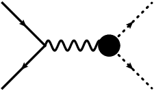
The unpolarized center-of-mass cross section is then
| (11) |
Note that an identical formula can be used for the reaction , and that we are neglecting masses and Cabbibo–Kobayashi–Maskawa mixing. In principle these subprocesses are formally suppressed with respect to the pure GB elastic scattering in this channel (longitudinal gauge boson fusion) whose amplitude is given by
| (12) |
where we have truncated at the partial wave, and is the partial wave for elastic scattering (see Appendix A). It is of order instead of found in Eq. (9).
However, this is again only the parton-level process. In the LHC environment, we need to take the parton distribution functions into account, and here a pair of fermions are more readily available than . It turns out that this process is dominant as will be shown numerically below in Section 4.
Convolving Eq. (11) with the pdfs as described earlier in Section 2.2, we obtain the proton-proton inclusive cross section to produce a pair of GBs as
| (13) |
To conclude this section, let us note that in the limit of vanishing hypercharge , custodial symmetry predicts a few relations
| (14) | |||||
so that our numerical computation for the reaction in Eq. (11) can be immediately used to estimate several others.
4 Numerical results and discussion
4.1 Parameters
The Weinberg angle in Eq. (4) corresponds to the tree-level radiation of a gauge boson, so it can be taken [18, 19] as (at the next order one should use the value at the pole, but this higher precision is irrelevant for us). Likewise, we take . With this, the auxiliary couplings in Eq. (4) are determined to be about and .
Once the generic parameters have been fixed, we can obtain the pertinent gauge boson–parton distribution functions in the effective boson approximation. The ones for the collisions, and from Eq. (3), are shown as the dashed and dotted curves in Fig. 3,

and those appropriate for a 6.5 TeV proton beam (the LHC run II operates at 13 TeV in center-of-mass energy) are shown as solid and dot-dashed curves in the same figure. One can clearly see that, at the same energy, it is more likely to split a vector boson from the proton at low , and less likely at moderately high (since the quark pdfs in the proton typically fall off as ).
Moving now to the parameters of the effective Lagrangian density in Eq. (1), the concurrent constraints on the value of from CMS and ATLAS [20] indicate, at , that , that is, around the Standard Model value 1, so that the leading order (LO) interaction strengths in the , and channels, being proportional to , are small and do not produce elastic- dynamically-generated states easily (inelastic are much more unconstrained as observed in Ref. [1]).
We resort to the NLO couplings to induce resonances in the unitarization process, taking as a first set , , at a scale TeV, and as a second set , , (also at TeV), with all other couplings set to zero. The first set produces an exemplary narrow isotensor resonance at around 2 TeV 11 1 Note that for this set and the QCD-like repulsive nature of the isotensor channel is reversed, so an isotensor pole is possible, while an isovector one becomes more difficult and violates causality in much of parameter space, see Fig. 22 of Ref. [1]. and the second set produces a narrow vector-isovector resonance (akin to a or a Higgs-composite model [21]) and a broad scalar-isoscalar one, both of which are around 2 TeV. Theses exemplary resonances can be clearly seen in the moduli of the amplitudes shown in Fig. 4 (for explicit expressions of these amplitudes, we refer to Ref. [1]).


From the parameter space of the effective field theory reported in Ref. [1] we have chosen these two sets because the resonances generated have a mass close to 2 TeV, so they would be clear candidates to explain the putative ATLAS resonances.
4.2 Estimate of the cross sections


First, let us see what the effective boson approximation of Section 2 produces for the case of an isotensor resonance. In Fig. 5, we show the differential cross section for the production of a pair of in both electron-positron and proton-proton collisions. We have summed up the individual cross sections with and in the initial state. We use the parameter set that generates an isotensor resonance (able to simultaneously explain an excess in all , and channels) which is visible in the curves. One sees that the peak differential cross section at the LHC run-I with a 8 TeV total energy is well below 0.1 fb/TeV2. It is increased by one order of magnitude at the 13 TeV LHC run-II operational energy and at a 3 TeV electron-positron collider, and reaches 1 fb/TeV2 at a 5 TeV lepton collider.
Next, we turn to the case of an isovector resonance. In this case, the mechanism shown in Fig. 1 is much less important than the mechanism, described in Section 3, of an intermediate boson. This can be clearly seen in the left panel of Fig. 6 which was calculated using the second parameter set.


The right panel of Fig. 6 shows the inclusive cross section in the proton-proton collisions through an intermediate boson in the presence of a vector-isovector resonance generated using the second parameter set. If we switch off the resonance, i.e., with , the cross section will drop exponentially without any enhancement at around 2 TeV.

4.3 Summary and conclusions
It appears that the expected production rate of resonances stemming purely from the EWSBS is near and below the CMS reach with the statistics accumulated in run I at 8 TeV (see Fig. 7). We do find parameter sensitivity. For example, if the values of , are modified to , , the cross section at the (approximately) 2 TeV peak drops by a factor 2, and falls way below CMS’s exclusion reach.
It then remains hard to believe, though open, that the ATLAS excess at 2 TeV in the diboson channel can be attributed to purely EWSBS-resonances alone. Our argumentation is rather model-independent as we rely on unitarized effective field theory without commitment to specific underlying BSM mechanisms. 22 2 Using different unitarization methods can result in some model dependence, however, the glossary features for the dynamically generated electroweak resonances remain the same as discussed in Ref. [1].
On the other hand, we have not examined fermion couplings, and new physics that couples intensely to the QCD partons in the initial state remains an option as the cross section would be increased respect to the -suppressed rate to produce an intermediate boson. Low-energy flavor tests however challenge such an interpretation, as remarked by other authors. We are currently executing an extended investigation of the generic EWSBS sector coupled to fermions in a symmetry-respecting effective Lagrangian in the framework of another collaboration. Another alternative interpretation of the data has been recently proposed [22] in which an additional boson has escaped detection (in spite of the already large cross section).
Run II at 13 TeV will improve the situation regarding the exclusion of purely electroweak-symmetry breaking sector resonances because the cross section (largely thanks to much increased parton luminosity) will increase substantially, as seen in Fig. 6. Right now, there is just not enough sensitivity. Another interesting way of increasing the cross section, as we showed in Fig. 5, is to proceed to a lepton collider where the initial state pointlike fermions are much more energetic, or to construct a higher-energy hadron collider (the longitudinal production mechanism becomes competitive around 100 TeV) such as the second phase of the proposed Circular Electron-Positron Collider–Super Proton-Proton Collider (CEPC-SPPC) [23].
For the time being, we conclude that longitudinal collinear radiation is not a competitive production mechanism at present energies, becoming important for an TeV pp collider, and that the ATLAS excess, if not a statistical fluctuation as the collaboration keeps as working hypothesis, does not easily fit as a resonance purely coupled to the electroweak gauge bosons, rather independently of model considerations.
Acknowledgments
We warmly thank intense discussions and information exchange with J. J. Sanz Cillero and D. Espriu. We are grateful to U.-G. Meißner for a careful reading of the manuscript. This work is partially supported by the Spanish Excellence Network on Hadronic Physics FIS2014-57026-REDT, by grants UCM:910309, MINECO:FPA2011-27853-C02-01, MINECO:FPA2014-53375-C2-1-P, by DFG and NSFC through funds provided to the Sino-German CRC 110 “Symmetries and the Emergence of Structure in QCD” (NSFC Grant No. 11261130311) and by NSFC (Grant No. 11165005).
Appendix A Strongly interacting amplitudes and form factors
A.1 Isospin relations
The isospin and partial wave expansions for the scattering amplitudes in the isospin basis can be found in [1]; here we show a few equations of interest.
For the process , the initial vector bosons are . Thus, the relevant rescattering process is , whose amplitude is given by
| (15) |
which can be easily obtained from the isospin relations noticing . The initial vector bosons are for the process , and we have
| (16) |
While for the processes and , we have the amplitudes
| (17) |
and
| (18) |
respectively. If the vector boson pair is charged, i.e. , there is no contribution from the isospin scalar channel. For such a process as , the relevant scattering amplitude is
| (19) |
These scattering amplitudes are related to the partial wave ones by
| (20) |
where if all the particles in the initial and final states are identical, and otherwise. The unitarized expressions for the partial wave amplitudes are shown next in Appendix A.2.
If we truncate the summation over at , the invariant amplitudes can be reconstructed easily from the partial waves by
| (21) |
A.2 Unitarization procedure: IAM
In this section, we will briefly describe our unitarization procedure, the Inverse Amplitude Method (IAM) [11, 1].
The effective-theory, partial-wave projected amplitudes satisfy on their right-hand cut (RC) unitarity only perturbatively, reading with and denoting LO and NLO only, respectively. This follows easily from their generic structure
| (22) |
and the field theory computation of the constants , and .
A complex- analysis of the elastic partial-wave scattering amplitude yields an exact, but not too useful, dispersion relation for , and that for is not necessary because it is known everywhere from perturbation theory. A useful technique is to apply a dispersive analysis to the following auxiliary function,
| (23) |
This has the same analytic structure as but for poles (at the zeroes of ) that have been treated in the past [24] and concluded to be irrelevant for the physical region of . Moreover, , , and on the RC one has . The twice-subtracted dispersion relation for this function, sufficient for one-channel problems, reads
| (24) |
where is a ultraviolet cutoff. With the definition of given in Eq. (23), one can compute the elastic-RC integral exactly since there. This is dominant because it is the nearest complex-plane singularity to the physical boundary which is the upper edge of the RC in the first Riemann sheet.
Because the left-hand cut (LC) integral cannot be obtained exactly, it is customarily computed in perturbation theory. As discussed in Ref. [1], it is a very reasonable approximation to take
| (25) |
which leads to
| (26) |
This approximate integral equation is solved by . In the above derivation, the only used approximations are the absence of poles in and the perturbative treatment of the LC integral. Therefore, from the definition of the in Eq. (23) we get the partial-wave amplitude in IAM as
| (27) |
This IAM amplitude has the proper analytic structure and makes poles on the second Riemann sheet possible which correspond to dynamically generated resonances. Elastic unitarity is satisfied by construction, and the amplitude is also scale independent. Furthermore, expanding at low energies, the IAM amplitude coincides with the one in chiral perturbation theory up to NLO,
| (28) |
Watson’s final state theorem [25] guarantees that the phase of the form factor for represented as the black blob in Fig. 2 is the same as that of the elastic scattering amplitude, and any resonance pole of the scattering amplitude also appears in the form factor at the same position in the complex -plane. Together with the normalization of the vector form factor we find that the form factor consistent with the IAM is given by
| (29) |
This construction agrees with the perturbative expansion, has the correct unitarity cut, and shares phase with the corresponding scattering amplitude in the same channel. Figure 8 shows the vector-isovector form factor necessary for Eq. (13) with the parameter set , , .

Appendix B Kinematics of the effective boson approximation
In this appendix we collect some useful relations among the kinematic variables of section 2. Specifically, we relate the transverse momenta of the vector mesons in the final state to the Mandelstam variables and the center-of-mass scattering angle which appear in the scattering amplitudes.
Let us start from the Mandelstam variable for the two-body scattering process . For the case and ,
| (B.1) |
where is the modulus of the momentum in the center-of-mass frame of the initial (or final) state.
On the other hand, we can decompose , which is the momentum for particle in the center-of-mass frame of the system, into , where and are the components parallel and perpendicular to , respectively. Since and are collinear with the beam direction in the effective approximation valid at high energies,
| (B.2) | |||||
where is the transverse momentum of particle in the laboratory frame. To obtain the second equality, we have used the fact that the perpendicular component of is invariant under the Lorentz boost from the laboratory frame to the cm frame. From Eqs. (B.1) and (B.2), we obtain the following relations for assuming and ,
| (B.3) |
For the case that all the particles are massless, then , and
| (B.4) |
where we have used .
References
- [1] R. L. Delgado, A. Dobado and F. J. Llanes-Estrada, Phys. Rev. Lett. 114, 221803 (2015) [arXiv:1408.1193 [hep-ph]]; R. L. Delgado, A. Dobado and F. J. Llanes-Estrada, Phys. Rev. D 91, 075017 (2015) [arXiv:1502.04841 [hep-ph]].
- [2] R. L. Delgado, A. Dobado and F. J. Llanes-Estrada, J. Phys. G 41, 025002 (2014) [arXiv:1308.1629 [hep-ph]]; R. L. Delgado, A. Dobado and F. J. Llanes-Estrada, JHEP 1402, 121 (2014) [arXiv:1311.5993 [hep-ph]]; R. L. Delgado, A. Dobado, M. J. Herrero and J. J. Sanz-Cillero, JHEP 1407, 149 (2014) [arXiv:1404.2866 [hep-ph]].
- [3] R. Alonso, I. Brivio, B. Gavela, L. Merlo and S. Rigolin, JHEP 1412, 034 (2014) [arXiv:1409.1589 [hep-ph]].
- [4] W. Kilian, T. Ohl, J. Reuter and M. Sekulla, Phys. Rev. D 91, 096007 (2015) [arXiv:1408.6207 [hep-ph]].
- [5] G. Buchalla, O. Cata, A. Celis and C. Krause, arXiv:1504.01707 [hep-ph].
- [6] J. M. Cornwall, D. N. Levin and G. Tiktopoulos, Phys. Rev. D 10, 1145 (1974) [Phys. Rev. D 11, 972 (1975)]; C. E. Vayonakis, Lett. Nuovo Cim. 17, 383 (1976); M.S. Chanowitz and M.K. Gaillard, Nucl. Phys. 261, 379 (1985); G.J. Gounaris, R. Kogerler and H. Neufeld, Phys. Rev. D 34, 3257 (1986).
- [7] A. Dobado J. R. Peláez Nucl. Phys. B425, 110 (1994); Phys. Lett. B 329, 469 (1994) (Addendum, ibid, B335, 554 (1994); C. Grosse-Knetter and I.Kuss, Z. Phys. C 66, 95 (1995); H. J. He, Y. P. Kuang and X. Li, Phys. Lett. B 329, 278 (1994).
- [8] G. Aad et al. [ATLAS Collaboration], arXiv:1506.00962 [hep-ex].
- [9] D. Espriu and F. Mescia, Phys. Rev. D 90, 015035 (2014) [arXiv:1403.7386 [hep-ph]]; D. Espriu, F. Mescia and B. Yencho, Phys. Rev. D 88, 055002 (2013) [arXiv:1307.2400 [hep-ph]]; D. Espriu and B. Yencho, Phys. Rev. D 87, 055017 (2013) [arXiv:1212.4158 [hep-ph]].
- [10] T. N. Truong, Phys. Rev. Lett. 61, 2526 (1988).
- [11] A. Dobado, M. J. Herrero and T. N. Truong, Phys. Lett. B 235, 134 (1990); A. Dobado and J.R. Peláez, Phys. Rev. D 47, 4883 (1993); Phys. Rev. D 56, 3057 (1997).
- [12] P. Arnan, D. Espriu and F. Mescia, arXiv:1508.00174 [hep-ph].
- [13] V. Khachatryan et al. [CMS Collaboration], JHEP 1408, 173 (2014) [arXiv:1405.1994 [hep-ex]].
- [14] S. Dawson, Nucl. Phys. B 249, 42 (1985).
- [15] A. Dobado and M. J. Herrero, Phys. Lett. B 233, 505 (1989).
- [16] J. F. Owens, A. Accardi and W. Melnitchouk, Phys. Rev. D 87, 094012 (2013) [arXiv:1212.1702 [hep-ph]].
- [17] A. Dobado, M. J. Herrero, J. R. Peláez and E. Ruiz Morales, Phys. Rev. D 62, 055011 (2000) [hep-ph/9912224].
- [18] K. A. Olive et al. [Particle Data Group], Chin. Phys. C 38, 090001 (2014).
- [19] W. J. Marciano, AIP Conf. Proc. 542, 48 (2000) [hep-ph/0003181].
- [20] The ATLAS collaboration [ATLAS Collaboration], ATLAS-CONF-2014-009, ATLAS-COM-CONF-2014-013; also the CMS Collaboration report CMSPASHIG-14-009.
- [21] D. Barducci, H. Cai, S. De Curtis, F. J. Llanes-Estrada and S. Moretti, Phys. Rev. D 91, 095013 (2015) [arXiv:1501.01830 [hep-ph]].
- [22] J. A. Aguilar-Saavedra, arXiv:1506.06739 [hep-ph].
- [23] M. Ahmad et al. [CEPC-SPPC Study Group], CEPC-SPPC Preliminary Conceptual Design Report, IHEP-CEPC-DR-2015-01.
- [24] A. Gomez Nicola, J. R. Peláez and G. Ríos, Phys. Rev. D 77, 056006 (2008) [arXiv:0712.2763 [hep-ph]].
- [25] K. M. Watson, Phys. Rev. 88, 1163 (1952).