A Learning-Based Approach to Caching in Heterogenous Small Cell NetworksThanks: B. N. Bharath is with People’s Education Society Institute of Technology, Bangalore South Campus, INDIA, E-mail: bharathbn@pes.edu. K. G. Nagananda is with People’s Education Society University, INDIA, E-mail: kgnagananda@pes.edu. H. Vincent Poor is with Princeton University, New Jersey, USA, E-mail: poor@princeton.edu

The advent of multimedia-capable devices at economical costs has triggered the growth of wireless data traffic at an unprecedented rate. This trend is likely to continue, requiring wireless service providers to reevaluate design strategies for the next generation wireless infrastructure [1]. A promising approach to address this problem is to deploy small cells that can offload a significant amount of data from a macro base station (BS) [2]. Doing so, it is expected to lead to cost-effective integration of the existing WiFi and cellular technologies with improved performance of peak data traffic steering policies [3]. However, a potential shortcoming of the small cell infrastructure is that, during peak traffic hours, the backhaul link-capacity requirement to support data traffic is enormously high [4]. Also, the cost incurred in deploying a high capacity backbone network for small cells can be quite high. Therefore, small cell-based solutions alone will not suffice to efficiently solve the quality of service requirements associated with peak traffic demands.

A noteworthy development in this direction is to improve the accessibility of data content to users by storing the most popular data files in the local caches (intermediate servers such as gateways, routers, etc.) of small cell BSs, with the objective of reducing the peak traffic rates. This is commonly referred to as “caching” and has attracted significant attention [5] - [8]. In the next subsection we mention a few references, which although by no means exhaustive, fairly indicate the scope and trend of research on caching.

In this section, we present the system model followed by the main problem addressed in the paper. The notation used in the rest of the paper is as follows: $\Phi_{u}$, $\Phi_{s}$ and $\Phi_{b}$ ($\lambda_{u}$, $\lambda_{s}$ and $\lambda_{b}$) denote the points (densities) corresponding to the user, SBSs and BS, respectively; $k_{x}$ denotes the number of requests in $[0,\tau]$ by the user at $x$; $X_{x}^{(l)}$ denotes the $l^{\text{th}}$ request of the user $x$; $\lambda_{r}$ is the average number of requests per unit time. A heterogenous cellular network is considered where the set $\Phi_{u}\subseteq\mathbb{R}^{2}$ of users, the set $\Phi_{b}\subseteq\mathbb{R}^{2}$ of BSs, and the set $\Phi_{s}\subseteq\mathbb{R}^{2}$ of SBSs are distributed according to independent PPPs with density $\lambda_{u}$, $\lambda_{b}$ and $\lambda_{s}$, respectively, in the two-dimensional space [41]. Each user independently requests a data-file of size $B$ bits from the set $\mathcal{F}\triangleq\{f_{1},f_{2},\ldots,f_{N}\}$; the popularity of data files is specified by the distribution $\mathcal{P}\triangleq\{p_{1},\ldots,p_{N}\}$, where $\sum_{i=1}^{N}p_{i}=1$ and is assumed to be stationary across time. In a typical heterogenous cellular network, the BS fetches a file using its backhaul link to serve a user. During peak data traffic hours, this results in an information-bottleneck both at the BS as well as in its backhaul link. To alleviate this problem, caching the most popular files (either at the user nodes or at SBSs) is proposed. The requested file will be served directly by one of the neighboring SBSs depending on the availability of the file in its local cache. The performance of caching depends on the density of SBS nodes, cache size, users’ request rate, and the caching strategy. It is assumed that the SBS can cache up to $M$ files, each of length $B$ bits. Each SBS in $\Phi_{s}$ caches its content in an independent and identically distributed (i.i.d.) fashion by generating $M$ indices distributed according to $\Pi\triangleq\{\pi_{i}:f_{i}\in\mathcal{F},~i=1,2,\ldots,N\}$, $\sum_{i=1}^{N}\pi_{i}=1$ (see [19]). One way of generating this is to roll an $N$ sided die $M$ times in an i.i.d. fashion, where the outcomes correspond to the index of the file to be cached. Although this approach is suboptimal, it is mathematically tractable and the corresponding time complexity serves as a lower bound, albeit pessimistic, for optimal strategies.

We now present a simple communications protocol to determine the set of neighboring SBS nodes for any user in $\Phi_{u}$. Essentially, we let each SBS at location $y\in\Phi_{s}$ communicate with a user at location $x\in\Phi_{u}$ if $\|y-x\|<\gamma$, ($\gamma>0$); this condition determines the communication radius. In this protocol, we have ignored the interference constraint. The set of neighbors of the user at location $x$ is denoted

In this section, we present two methods for estimating the popularity profile and provide the corresponding training time analyses. The efficiency of the estimate $\hat{\mathcal{P}}$ of the popularity profile depends on the number of available data samples, which in turn is related to the number of requests made by the users. We first obtain an expression for the estimate of the popularity profile. We then study, in Section III-A, the minimum training time in obtaining the samples to achieve a desired estimation accuracy $\epsilon>0$. Finally, in Section III-B, we employ the TL-based approach to improve the bound on the training time. We begin with the definition of the request model.

In the previous sections, no structure was imposed on the popularity profile. In practice, the popularity profile is modeled using a parametric family of distributions such as the Zipf distribution [38], which, with a one-dimensional parameter $\Theta\in\mathbb{R}$, is specified by ${p}_{\Theta,i}=\frac{{1/i^{\Theta}}}{\sum_{j=1}^{N}{1/j^{\Theta}}},i=1,2,\ldots,N$. To obtain an estimate of the Zipf distribution it suffices to find the parameter $\Theta$; estimating a single parameter requires fewer samples which can potentially reduce the training time. We now derive bounds on the training time when the popularity profile belongs to a parametric family of distributions. We begin with the following assumption:
Assumption 1: Let the family of parametrized popularity distributions be defined by $\mathcal{P}=\{\mathcal{P}_{\Theta}:\Theta\subseteq[a,b]^{d},a<b\}$. Further, for all $\Theta\subseteq[a,b]^{d}$, $\mathcal{P}_{\Theta}$ satisfies $\sum_{i=1}^{N}\|{\partial}_{\Theta}{p}_{\Theta,i}\|_{2}<C$, where $C<\infty$ is independent of $N$, and $\partial_{\Theta}{p}_{\Theta,i}\in\mathbb{R}^{d}$ denotes the sub-differential of ${p}_{\Theta,i}$. For example, the Zipf distribution ${p}_{\theta,i}=\frac{{1/i^{\alpha}}}{\sum_{j=1}^{N}{1/j^{\alpha}}},i=1,2,\ldots,N$ satisfies this property.

Let the true underlying parameter be $\Theta:=\{\Theta_{1},\ldots,\Theta_{d}\}$. Note that $\Theta_{j}\in[a,b]$ for all $j=1,2,\ldots,d$. Let the BS observe $n_{p}$ (number of requests) i.i.d samples $(X_{t,1},X_{t,2},\ldots,X_{t,n_{p}})\in\mathcal{X}_{t}^{n_{p}}$ drawn from the distribution $\mathcal{P}_{\Theta}$. Also, let $\hat{\Theta}_{n_{p}}^{(i)}:=\left(\hat{\Theta}_{n_{p},i,1},\hat{\Theta}_{n_{p},i,2},\ldots,\hat{\Theta}_{n_{p},i,d}\right)\in\mathbb{R}^{d}$, $i=1,2,\ldots,n_{p}$ denote the estimate of $\Theta$, based on a single observation, i.e., $\hat{\Theta}_{n_{p}}^{(i)}=f(X_{t,i})$, $i=1,2,\ldots,n_{p}$, where $f:\mathcal{X}_{t}\rightarrow[a,b]^{d}$ is an unbiased estimator of $\Theta$. In the above, $n_{p}$ denotes the number of requests made by the users corresponding to the BS $z$ in a time interval of $[0,\tau]$. Since $f(\cdot)$ is an unbiased estimator of $\Theta$, we have $\mathbb{E}\left\{\hat{\Theta}_{n_{p}}^{(i)}|\Theta\right\}=\Theta$ for all $i=1,2,\ldots,n_{p}$. The estimate of $\Theta$ using $n_{p}$ samples is obtained as follows:

Note that $\hat{\Theta}_{n_{p}}:=(\hat{\Theta}_{n_{p},1},\hat{\Theta}_{n_{p},2},\ldots,\hat{\Theta}_{n_{p},d}),$ is also an unbiased estimator of $\Theta$, i.e., $\mathbb{E}\left\{\hat{\Theta}_{n_{p}}|\Theta,n_{p}\right\}=\Theta$. The following theorem provides a bound on the time complexity for a family of parameterized popularity profile satisfying Assumption 1.

In this section, we provide numerical results and derive insights into the analyses carried out in the previous sections. The parameter values used in our calculations are as follows: $B=10^{7}~\text{bits}$, $R_{0}=10^{6}~\text{bits/s}$, $\gamma=100$m, $\lambda_{u}=0.001~\text{nodes}/m^{2}$, $\lambda_{r}=1/360~\text{requests/s}$, $\lambda_{s}=10^{-5}~\text{nodes}/m^{2}$, $\delta=0.02$, $R=2$ Km, $m=10^{5}$ samples, $\beta_{e}=0.6$ and $\beta_{l}=0.2$. $\epsilon$ is chosen as a fraction of a lower bound on the offloading loss, i.e., $\mathcal{T}(\Pi,\mathcal{P})\geq\frac{B}{R_{0}}\exp\{-\lambda_{s}\pi\gamma^{2}\}$. In particular, $\epsilon=\text{fraction}\times\frac{B}{R_{0}}\exp\{-\lambda_{s}\pi\gamma^{2}\}$. Further, $\|\mathcal{P}-\mathcal{Q}\|_{\infty}=0.1\left(\frac{\epsilon R_{0}}{2BN}\right)$ which for the above parameters is of the order of $10/N$.

Fig. 1 shows a plot of the lower bounds on the training duration obtained in Theorems 2 and 3 as functions of the support $N$. It is seen that, for $N\leq 70$ the TL-based approach provides significant performance improvement. However, for $N>70$, the performance of the TL-based approach degrades compared to the approach that uses only the source domain samples (and, hence, can be called agnostic). This suggests that for larger values of $N$, the estimate of the popularity profile obtained using (21) performs poorly due to incorrect fusion of the estimates obtained from source and target domains.

Fig. 2 shows the plots of the lower bound in Theorem 4 corresponding to the estimate obtained by a fixed linear combination of the source and target estimates (see (21)). As seen in the figure, this does not bring any performance improvement and in fact sometimes performs poorly compared to the source domain agnostic approach. This is because the fixed linear combination does not have the flexibility to adapt to different realizations of the network, proving the sub-optimality of the estimate in (21) compared to that in (15). It is also seen that the coefficients used in the estimate that adapts to the varying realizations of the network as in (21) is beneficial.

Fig. 3 shows a plot similar to that in Fig. 1 but with $N=10$ and varying $m$. It can be seen that the TL-based approach performs better for all $m\geq 1000$ demonstrating its applicability in practice. As seen, the performance is better for higher values of the fraction which corroborates intuition. Fig. 4 also shows a plot of time duration versus $m$ for a fixed $N=10$. It can be seen that the estimate in (21) outperforms the agnostic approach; however, this is observed at very high values of source domain samples ($m=10500$ and $m=16000$ for $\text{fraction}=0.5$ and $\text{fraction}=0.4$, respectively). Thus, although the TL-based approach using the estimate (21) has some benefits, it is not desirable for practical applications.

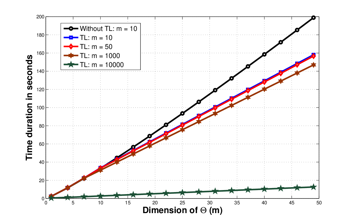
The main benefits of the TL-based approach are shown in Fig. 5 for the parametric family of popularity profiles. It can be seen that the TL-based approach performs significantly better than the source domain agnostic approach for values of $m$ as low as $10$. This is because the number of parameters to be estimated scales with the dimension of $\Theta$ rather than with the support. In particular, as $d$ increases the training duration also increases, which is quite expected. However, the delay scales only linearly in $d$ as compared to quadratic scaling experienced with the nonparametric method.

The popularity profile for caching in distributed heterogenous cellular networks was estimated at BS using the available instantaneous demands from users in a time interval $[0,\tau]$. We showed that a training time $\tau$ to achieve an $\epsilon>0$ difference between the achieved cost and the optimal cost was finite, provided the user density was greater than a threshold; $\tau$ was shown to scale as square of the support of the popularity profile. A TL-based approach was proposed to estimate the popularity profile, and a condition was derived under which it performed better than the target domain sample only based approach. Although TL-based approach performs better, the error that is achieved in (24) depends on $\|\mathcal{P}-\mathcal{Q}\|_{\infty}$, suggesting that lower the distance between the two distributions better the TL scheme performs. From Proposition 1, the benefits of using target domain samples can only be realized with the knowledge of the distance $\|\mathcal{P}-\mathcal{Q}\|_{\infty}$. The main benefit of the TL-based approach is recognized when the popularity profile is modeled using a parametric family of distributions. In this case, the delay is independent of $N$ and scales only linearly with the dimension of the distribution parameter. In practice, caching depends on several factors such as the scheduling scheme used, which in turn depends on the channel conditions, QoS requirements, etc. An important assumption that we make is that if the requested file is present in one (or more) of the neighboring SBSs, the transmissions are scheduled within a tolerable time frame. In the case of caching, this time duration could be slightly relaxed, and can be thought of as an abstraction of the scheduling scheme employed. If the file is not present, regardless of the scheduling policy, the file cannot be served locally. Hence, the approach that we have leads to a lower bound, albeit pessimistic, on the training time. Thus, even under pessimistic situations, the training time scales as $N^{2}\log N$ for achieving an offloading loss that is $\epsilon>0$ away from the optimal offloading loss.

K. G. Nagananda would like to thank Chandra R. Murthy, at the Indian Institute of Science, for providing the lab space during the course of this work. The work of H. Vincent Poor was supported in part by the U. S. National Science Foundation under Grant CNS-1456793. The authors thank the anonymous referees for their comments and suggestions.

References

- [1] A. Furuskar, J. Charles, M. Frodigh, S. Jeux, M. Sayed Hassan, A. Saadani, A. Stidwell, J. Soder, and B. Timus, “Refined statistical analysis of evolution approaches for wireless networks,” IEEE Trans. Wireless Commun., vol. 14, no. 5, pp. 2700 – 2710, May 2015.
- [2] S.-F. Chou, T.-C. Chiu, Y.-J. Yu, and A.-C. Pang, “Mobile small cell deployment for next generation cellular networks,” in Proc. IEEE Global Commun. Conf., Dec. 2014, pp. 4852–4857.
- [3] M. Bennis, M. Simsek, A. Czylwik, W. Saad, S. Valentin, and M. Debbah, “When cellular meets WiFi in wireless small cell networks,” IEEE Commun. Magazine, vol. 51, no. 6, pp. 44–50, Jun. 2013.
- [4] J. Kim, C. Jeong, H. Yu, and J. Park, “Areal capacity limit on the growth of small cell density in heterogeneous networks,” in Proc. IEEE Global Commun. Conf., Dec. 2014, pp. 4263–4268.
- [5] Y.-B. Lin, W.-R. Lai, and J.-J. Chen, “Effects of cache mechanism on wireless data access,” IEEE Trans. Wireless Commun., vol. 2, no. 6, pp. 1247–1258, Nov. 2003.
- [6] E. Baştuğ, M. Bennis, and M. Debbah, “Living on the edge: The role of proactive caching in 5G wireless networks,” IEEE Commun. Magazine, vol. 52, no. 8, pp. 82–89, Aug. 2014.
- [7] H. R. Sadjadpour, “A new design for Information Centric Networks,” in Proc. Conf. Inf. Sciences Syst., Mar. 2014, pp. 1–6.
- [8] U. Niesen, D. Shah, and G. W. Wornell, “Caching in wireless networks,” IEEE Trans. Inf. Theory, vol. 58, no. 10, pp. 6524–6540, Oct. 2012.
- [9] J.-H. Hu, G. Feng, and K. Yeung, “Hierarchical cache design for enhancing TCP over heterogeneous networks with wired and wireless links,” IEEE Trans. Wireless Commun., vol. 2, no. 2, pp. 205–217, Mar. 2003.
- [10] X. Wang, M. Chen, T. Taleb, A. Ksentini, and V. Leung, “Cache in the air: exploiting content caching and delivery techniques for 5G systems,” IEEE Trans. Wireless Commun., vol. 52, no. 2, pp. 131–139, Feb. 2014.
- [11] N. Golrezaei, P. Mansourifard, A. F. Molisch, and A. G. Dimakis, “Base-station assisted device-to-device communications for high-throughput wireless video networks,” IEEE Trans. Wireless Commun., vol. 13, no. 7, pp. 3665–3676, Jul. 2014.
- [12] G. Lee, I. Jang, S. Pack, and X. Shen, “FW-DAS: Fast wireless data access scheme in mobile networks,” IEEE Trans. Wireless Commun., vol. 13, no. 8, pp. 4260–4272, Aug. 2014.
- [13] K. Poularakis, G. Iosifidis, and L. Tassiulas, “Approximation algorithms for mobile data caching in small cell networks,” IEEE Trans. Commun., vol. 62, no. 10, pp. 3665–3677, Oct. 2014.
- [14] C. Fang, F. Yu, T. Huang, J. Liu, and Y. Liu, “A survey of energy-efficient caching in information-centric networking,” IEEE Commun. Magazine, vol. 52, no. 11, pp. 122–129, Nov. 2014.
- [15] H. Asaeda, K. Matsuzono, and T. Turletti, “Contrace: a tool for measuring and tracing content-centric networks,” IEEE Commun. Magazine, vol. 53, no. 3, pp. 182–188, Mar. 2015.
- [16] R. Pedarsani, M. A. Maddah-Ali, and U. Niesen, “Online coded caching,” in Proc. IEEE Int. Conf. Commun., Jun. 2014, pp. 1878–1883.
- [17] Y. Guan, Y. Xiao, H. Feng, C.-C. Shen, and L. J. Cimini, “MobiCacher: Mobility-aware content caching in small-cell networks,” in Proc. IEEE Global Commun. Conf., Dec. 2014, pp. 4537–4542.
- [18] A. Pyattaev, O. Galinina, S. Andreev, M. Katz, and Y. Koucheryavy, “Understanding practical limitations of network coding for assisted proximate communication,” IEEE J. Select. Areas Commun., vol. 33, no. 2, pp. 156–170, Feb. 2015.
- [19] M. Ji, G. Caire, and A. F. Molisch, “Optimal throughput-outage trade-off in wireless one-hop caching networks,” in Proc. IEEE Int. Symp. Inf. Theory, Jul. 2013, pp. 1461–1465.
- [20] N. Golrezaei, A. G. Dimakis, and A. F. Molisch, “Wireless device-to-device communication with distributed caching,” in Proc. IEEE Int. Symp. Inf. Theory, Jul. 2012, pp. 2781–2785.
- [21] M. Ji, G. Caire, and A. F. Molisch, “Fundamental limits of distributed caching in D2D wireless networks,” in Proc. IEEE Inf. Theory Workshop, Sep. 2013, pp. 1–5.
- [22] ——, “Fundamental limits of caching in wireless D2D networks,” IEEE Trans. Inf. Theory, vol. 62, no. 2, pp. 849–869, Jan. 2016.
- [23] E. Baştuğ, M. Bennis, M. Kountouris, and M. Debbah, “Cache-enabled small cell networks: modeling and tradeoffs,” EURASIP J. Wireless Commun. Net., vol. 2015:41, Feb. 2015.
- [24] C. Yang, Y. Yao, Z. Chen, and B. Xia, “Analysis on cache-enabled wireless heterogeneous networks,” IEEE Trans. Wireless Commun., vol. 15, no. 1, pp. 131–145, Jan. 2015.
- [25] S. H. Chae, J. Y. Ryu, T. Q. S. Quek, and W. Choi, “Cooperative transmission via caching helpers,” in Proc. IEEE Global Commun. Conf., Dec. 2015.
- [26] S. Tamoor-ul Hassan, M. Bennis, P. H. J. Nardelli, and M. Latva-Aho, “Modeling and analysis of content caching in wireless small cell networks,” in Proc. IEEE Int. Symp. Wireless Commun. Syst., Aug. 2015.
- [27] L. Zhang, M. Xiao, G. Wu, and S. Li, “Efficient scheduling and power allocation for D2D-assisted wireless caching networks,” IEEE Trans. Commun., 2015, submitted.
- [28] J. Li, M. Xiao, W. Chen, and X. Liu, “Efficient video pricing and caching in heterogeneous networks,” IEEE Trans. Vehicular Tech., 2015, to appear.
- [29] M. A. Maddah-Ali and U. Niesen, “Fundamental limits of caching,” IEEE Trans. Inf. Theory, vol. 60, no. 5, pp. 2856–2867, May 2014.
- [30] U. Niesen, C. Beilken, and M. A. Maddah-Ali, “Coded caching with nonuniform demands,” in Proc. IEEE Conf. Comp. Commun. Workshop, Apr. 2014, pp. 221–226.
- [31] M. Maddah-Ali and U. Niesen, “Decentralized coded caching attains order-optimal memory-rate tradeoff,” IEEE/ACM Trans. Networking, vol. 23, no. 4, pp. 1029–1040, Aug. 2015.
- [32] N. Karamchandani, U. Niesen, M. A. Maddah-Ali, and S. N. Diggavi, “Hierarchical coded caching,” in Proc. IEEE Int. Symp. Inf. Theory, Jun. 2014, pp. 2142–2146.
- [33] P. Blasco and D. Gunduz, “Learning-based optimization of cache content in a small cell base station,” in Proc. IEEE Int. Conf. Commun., Jun. 2014, pp. 1897–1903.
- [34] ——, “Multi-armed bandit optimization of cache content in wireless infostation networks,” in Proc. IEEE Int. Symp. Inf. Theory, Jun. 2014, pp. 51–55.
- [35] A. Sengupta, S. Amuru, R. Tandon, R. M. Buehrer, and T. C. Clancy, “Learning distributed caching strategies in small cell networks,” in Proc. IEEE Int. Symp. Wireless Commun. Syst., Aug. 2014, pp. 917–921.
- [36] E. Baştuğ, M. Bennis, and M. Debbah, “Anticipatory caching in small cell networks: A transfer learning approach,” in Workshop Anticipatory Net., Germany, Sep. 2014.
- [37] ——, “A transfer learning approach for cache-enabled wireless networks,” in Int. Symp. Model. Opt. Mobile, Ad Hoc Wireless Net. (WiOpt), May 2015, pp. 161–166.
- [38] J. Llorca, A. M. Tulino, K. Guan, and D. C. Kilper, “Network-coded caching-aided multicast for efficient content delivery,” in Proc. IEEE Int. Conf. Commun., Jun. 2013, pp. 3557–3562.
- [39] N. Golrezaei, K. Shanmugam, A. Dimakis, A. Molisch, and G. Caire, “Femto caching: Wireless video content delivery through distributed caching helpers,” IEEE Trans. Inf. Theory, vol. 59, no. 12, pp. 8402–8413, Dec. 2013.
- [40] B. N. Bharath and K. G. Nagananda, “Caching with unknown popularity profiles in small cell networks,” in Proc. IEEE Global Commun. Conf., Dec. 2015. [Online]. Available: http://arxiv.org/pdf/1504.03632v1.pdf
- [41] F. Baccelli, M. Klein, M. Lebourges, and S. Zuyev, “Stochastic geometry and architecture of communication networks,” J. Telecom. Syst., vol. 7, no. 1, pp. 209–227, 1997.
- [42] V. Vapnik and A. Chervonenkis, “Theory of pattern recognition,” Moscow (in Russian), German Translation: Theorie der Zeichenerkennung, Akademie Verlag, Berlin, 1979.
- [43] L. Devroye, L. Gyorfi, and G. Lugosi, A Probability Theory of Pattern Recognition. Springer, 2014.
Appendix A Proof of Theorem 1
The first term in (2), , can be written as
where . In the above exposition, follows from the fact that the proposed random caching scheme is independent across users, is due to the fixed cache size (), and follows since is a PPP with mean , where is the number of SBSs in a circular area of radius . This completes the proof of Theorem 1.
Appendix B Proof of Theorem 2
For any , the inequality is proved, where . And, can be written as (see [42])
where , thus proving the inequality. Substituting for and from (4) we get , which can be upper bounded as follows: