Position-dependent power spectrum: a new
observable in the large-scale structure
Chi-Ting Chiang
![[Uncaptioned image]](1508.03256v1/siegel.png)
München 2015
Position-dependent power spectrum: a new
observable in the large-scale structure
Chi-Ting Chiang
Dissertation
an der Fakultät für Physik
der Ludwig–Maximilians–Universität
München
vorgelegt von
Chi-Ting Chiang
aus Taipei, Taiwan
München, den Abgabedatum
Erstgutachter: Prof. Dr. Eiichiro Komatsu
Zweitgutachter: Prof. Dr. Jochen Weller
Tag der mündlichen Prüfung: 22 June 2015
Zusammenfassung
In dieser Dissertation führe ich eine neue Observable der grossräumigen Struktur des Universums ein, das ortsabhängige Leistungsspektrum. Diese Größe bietet ein Mass für den “gequetschten” Limes der Dreipunktfunktion (Bispektrum), das heisst, eine Wellenzahl ist wesentlich kleiner als die beiden übrigen. Physikalisch beschreibt dieser Limes der Dreipunktfunktion die Modulation des Leistungsspektrums auf kleinen Skalen durch grossräumige Moden. Diese Modulation wird sowohl durch die Schwerkraft bewirkt als auch (möglicherweise) durch die kosmologische Inflation im frühen Universum.
Für die Messung teilen wir das Gesamtvolumen der Himmelsdurchmusterung, oder kosmologischen Simulation, in Teilvolumina ein. In jedem Teilvolumen messen wir die Überdichte relativ zur mittleren Dichte der Materie (oder Anzahldichte der Galaxien) und das lokale Leistungsspektrum. Anschliessend messen wir die Korrelation zwischen Überdichte und Leistungsspektrum. Ich zeige, dass diese Korrelation einem Integral über die Dreipunktfunktion entspricht. Wenn die Skala, an der das Leistungsspektrum ausgewertet wird (inverse Wellenzahl, um genau zu sein), viel kleiner als die Größe des Teilvolumens ist, dann ist das Integral über die Dreipunktfunktion vom gequetschten Limes dominiert.
Um physikalisch zu verstehen, wie eine grossräumige Dichtefluktuation das lokale Leistungsspektrum beeinflusst, wenden wir das Bild vom “unabhängigen Universum” (“separate universe”) an. Im Kontext der allgemeinen Relativitätstheorie kann eine langwellige Dichtefluktuation exakt durch eine Friedmann-Robertson-Walker-(FRW-)Raumzeit beschrieben werden, deren Parameter sich von der “wahren” FRW-Raumzeit unterscheiden und eindeutig von der Dichtefluktuation bestimmt werden. Die Modulation des lokalen Leistungsspektrums kann dann durch die Strukturbildung innerhalb der modifizierten FRW-Raumzeit beschrieben werden. Insbesondere zeige ich, dass die Dreipunktfunktion im gequetschten Limes durch diesen Ansatz einfacher und besser beschrieben wird als durch die herkömmliche Herangehensweise mittels Störungstheorie.
Diese neue Observable ist nicht nur einfach zu interpretieren (sie stellt die Antwort des lokalen Leistungsspektrums auf eine großskalige Dichtestörung dar), sie ermöglicht zudem die komplexe Berechnung der vollen Dreipunktsfunktion zu umgehen, weil das Leistungsspektrum genauso wie die mittlere Dichte wesentlich leichter als die Dreipunktsfunktion zu bestimmen sind.
Anschließend wende ich die gleiche Methodik auf die Daten der Himmelsdurchmustering SDSS-III Baryon Oscillation Spectroscopic Survey (BOSS) an, insbesondere den Data Release 10 CMASS Galaxienkatalog. Wie ich zeige, stimmt das in den wirklichen Daten gemessene ortsabhängige Leistungsspektrum mit den sogenannten “mock” (also simulierten) Galaxienkatalogen überein, die auf dem PTHalo-Algorithmus basieren und die räumlichde Verteilung der wirklichen Galaxien im statistischen Sinne möglichst genau beschreiben wollen. Genauer gesagt, liegen die Daten innerhalb der Streuung, die das ortsabhängige Leistungsspektrum zwischen den verschiedenen Realisierungen von “mock” Katalogen aufweist. Diese Streuung beträgt ca. 10% des Mittelewerts. In Kombination mit dem (anisotropen) globalen Leistungsspektrum der Galaxien sowie dem Signal im schwachen Gravitationslinseneffekt, benutze ich diese 10%-Messung des ortsabhängigen Leistungsspektrums, um den quadratischen Bias-Parameter der von BOSS gemessenen Galaxien zu bestimmen, mit dem Ergebnis (68% Vertrauensintervall).
Schließlich verallgemeinern wir die Analyse der Antwort des lokalen Leistungsspektrums auf eine Häufung von großräumigen Wellenlängenmoden, wobei . In Analogie zum vorherigen Fall, kann die resultierende Modulation des Leistungsspektrums mit der -Punktskorrelationsfunktion im Limes gequetschter Konfigurationen (so dass immer zwei Wellenlängen wesentlich länger sind als die anderen), gemittled über die auftretenden Winkel, in Verbindung gebracht werden. Mit Hilfe von Simulationen “unabhängiger Universen”, dass heißt -body-Simulationen in Anwesenheit von Dichtestörungen unendlicher Länge, vergleichen wir unsere semianalytischen Modelle, die auf dem Bild der unabhängigen Universen basieren, mit den vollständig nichtlinearen Simulationen bei bisher unerreichter Genauigkeit. Zudem testen wir die Annahme der gewöhnlichen Störungstheorie, dass die nichtlineare N-Punktskorrelationsfunktion vollständig durch das lineare Leistungsspektrum bestimmt ist. Wir finden bereits Abweichungen von 10% bei Wellenzahlen von für die Drei- bis Fünf-Punktskorrelationsfunktion bei Rotverschiebung . Dieses Ergebnis deutet darauf hin, dass die gewöhnlichye Störungstheorie nicht ausreicht um die Dynamik kollissionsloser Teilchen für Wellenzahlen größer als diese korrekt vorherzusagen, selbst wenn alle höheren Ordnungen in die Berechnung mit einbezogen werden.
Abstract
We present a new observable, position-dependent power spectrum, to measure the large-scale structure bispectrum in the so-called squeezed configuration, where one wavenumber, say , is much smaller than the other two, i.e. . The squeezed-limit bispectrum measures how the small-scale power spectrum is modulated by a long-wavelength scalar density fluctuation, and this modulation is due to gravitational evolution and also possibly due to the inflationary physics.
We divide a survey volume into smaller subvolumes. We compute the local power spectrum and the mean overdensity in each smaller subvolume, and then measure the correlation between these two quantities. We show that this correlation measures the integral of the bispectrum, which is dominated by the squeezed configurations if the wavenumber of the local power spectrum is much larger than the corresponding wavenumber of the size of the subvolumes. This integrated bispectrum measures how small-scale power spectrum responds to a long-wavelength mode.
To understand theoretically how the small-scale power spectrum is affected by a long-wavelength overdensity gravitationally, we use the “separate universe picture.” A long-wavelength overdensity compared to the scale of interest can be absorbed into the change of the background cosmology, and then the small-scale structure formation evolves in this modified cosmology. We show that this approach models nonlinearity in the bispectrum better than the traditional approach based on the perturbation theory.
Not only this new observable is straightforward to interpret (the response of the small-scale power spectrum to a long-wavelength overdensity), but it also sidesteps the complexity of the full bispectrum estimation because both power spectrum and mean overdensity are significantly easier to estimate than the full bispectrum.
We report on the first measurement of the bispectrum with the position-dependent correlation function from the SDSS-III Baryon Oscillation Spectroscopic Survey (BOSS) Data Release 10 CMASS sample. We detect the amplitude of the bispectrum of the BOSS CMASS galaxies at , and constrain their nonlinear bias to be (68% C.L.) combining our bispectrum measurement with the anisotropic clustering and the weak lensing signal.
We finally generalize the study to the response of the small-scale power spectrum to long-wavelength overdensities for . Similarly, this response can be connected to the angle-average -point function in the squeezed configurations where two wavenumbers are much larger than the other ones. Using separate universe simulations, i.e. -body simulations performed in the presence of an infinitely long-wavelength overdensity, we compare our semi-analytical models based on the separate universe approach to the fully nonlinear simulations to unprecedented accuracy. We also test the standard perturbation theory hypothesis that the nonlinear -point function is completely predicted by the linear power spectrum at the same time. We find discrepancies of 10% at for three- to five-point functions at . This result suggests that the standard perturbation theory fails to describe the correct dynamics of collisionless particles beyond these wavenumbers, even if it is calculated to all orders in perturbations.
Chapter 1 Introduction
1.1 Why study the position-dependent power spectrum of the large-scale structure?
The standard cosmological paradigm has been well developed and tested by the observations of the cosmic microwave background (CMB) and the large-scale structure. The inhomogeneities seen in the universe originate from quantum fluctuations in the early universe, and these quantum fluctuations were stretched to macroscopic scales larger than the horizon during the cosmic inflation [69, 132, 5, 99], which is the early phase with exponential growth of the scale factor. After the cosmic inflation, the hot Big-Bang universe expanded and cooled down, and the macroscopic inhomogeneities entered into horizon and seeded all the structures we observe today.
With the success of connecting the quantum fluctuations in the early universe to the structures we see today, the big questions yet remain: What is the physics behind inflation? Also, what is nature of dark energy, which causes the accelerated expansion in the late-time universe (see [57] for a review)? As the standard cosmological paradigm passes almost all the tests from the current observables, especially the two-point statistics of CMB and galaxy surveys, it is necessary to go to higher order statistics to obtain more information and critically test the current model. In particular, the mode coupling between a long-wavelength scalar density fluctuation and the small-scale structure formation receives much attention in the past few years. This coupling is due to the nonlinear gravitational evolution (see [17] for a review), and possibly the inflationary physics. Therefore, this provides a wonderful opportunity to test our understanding of gravity, as well as to probe the properties of inflation.
Traditionally, the -point function with is used to characterize the mode coupling. Specifically, if one is interested in the coupling between one long-wavelength mode and two short-wavelength modes, we measure the three-point correlation function or its Fourier counterpart, the bispectrum, in the so-called “squeezed configurations,” in which one wavenumber, say , is much smaller than the other two, i.e. .
In the simplest model for the primordial non-Gaussianity (see [27] for a review on the general primordial non-Gaussianities from various inflation models), the primordial scalar potential is given by
| (1.1) |
where is a Gaussian field and is a constant characterizing the amplitude of the non-Gaussianity, which encodes the properties of inflation. Note that assures . This simple model is known as the local-type primordial non-Gaussianity because depends locally on . The bispectrum of this local model is
| (1.2) |
where is the power spectrum of the primordial scalar potential and is its spectral index [88]. We can rewrite of this local model by fixing one wavenumber, say , as
| (1.3) |
where because of the assumption of homogeneity. apparently peaks at , so the local-type primordial non-Gaussianity is the most prominent in the squeezed-limit bispectrum.
Constraining the physics of inflation using the squeezed-limit bispectrum of CMB is a solved problem [87]. With the Planck satellite, the current constraint on the local-type primordial non-Gaussianity is (68% C.L.) using the temperature data alone and using the temperature and polarization data [128]. These are close to the best limits obtainable from CMB. To improve upon them, we must go beyond CMB to the large-scale structure, where observations are done in three-dimensional space (unlike CMB embedded on a two-dimensional sphere). Thus, in principle, the large-scale structure contains more information to improve the constraint on the physics of inflation.
Measuring the three-point function from the large-scale structure (e.g. distribution of galaxies), however, is considerably more challenging compared to CMB. From the measurement side, the three-point function measurements are computationally expensive. In configuration space, the measurements rely on finding particle triplets with the naive algorithm scaling as where is the number of particles. Current galaxy redshift surveys contain roughly a million galaxies, and we need 50 times as many random samples as the galaxies for characterizing the survey window function accurately. Similarly, in Fourier space, the bispectrum measurements require counting all possible triangle configurations formed by different Fourier modes, which is also computationally expensive. From the modeling side, galaxy surveys have more complicated survey selection function, which can bias the estimation (see e.g. [30]). Additionally, the nonlinear gravitational evolution of matter density field and the complexity of galaxy formation make it challenging to extract the primordial signal. The above difficulties explain why only few measurements of the three-point function of the large-scale structure have been reported in the literature [142, 55, 167, 82, 119, 109, 110, 105, 62, 67].
Since our main interest is to measure the three-point function of the squeezed configurations, there is a simpler way to sidestep all the above complexities of the three-point function estimation. As we stated, in the presence of the mode coupling between long- and short-wavelength modes, a long-wavelength density fluctuation modifies the small-scale structure formation, and so the observables become position-dependent. Figure 1.1 sketches the short-wavelength modes with (red) and without (blue) correlation with the long-wavelength mode. As a consequence, for example, the -point statistics and the halo mass function would depend on the local long-wavelength overdensity, or equivalently the position in space. Measurements of spatially-varying observables capture the effect of mode coupling, and can be used to test our understanding of gravity and the physics of inflation. A similar idea of measuring the shift of the peak position of the baryonic acoustic oscillation in different environments has been studied in [129].

In this dissertation, we focus on the position-dependent two-point statistics (see [32, 115] for the mass function). Consider a galaxy redshift survey or simulation. Instead of measuring the power spectrum within the entire volume, we divide the volume into many subvolumes, within which we measure the power spectrum. These power spectra of subvolumes vary spatially, and the variation is correlated with the mean overdensities of the subvolumes with respect to the entire volume. This correlation measures an integral of the bispectrum (or the three-point function in configuration space), which represents the response of the small-scale clustering of galaxies (as measured by the position-dependent power spectrum) to the long-wavelength density perturbation (as measured by the mean overdensity of the subvolumes).
Not only is this new observable, position-dependent power spectrum, of the large-scale structure conceptually straightforward to interpret, but it is also simpler to measure than the full bispectrum, as the machineries for the two-point statistics estimation are well developed (see [56] for power spectrum and [91] for two-point function) and the measurement of the overdensity is simple. In particular, the computational requirement is largely alleviated because we explore a subset of the three-point function corresponding to the squeezed configurations. More precisely, in Fourier space we only need to measure the power spectrum, and in configuration space the algorithm of measuring the two-point function by finding particle pairs scales as for the entire volume with being the number of subvolumes. In addition, for a fixed size of the subvolume, the measurement depends on only one wavenumber or one separation, so estimating the covariance matrix is easier than that of the full bispectrum from a realistic number of mock catalogs. The position-dependent power spectrum can thus be regarded as a useful compression of information of the squeezed-limit bispectrum.
As this new observable uses basically the existing and routinely applied machineries to measure the two-point statistics, one can easily gain extra information of the three-point function, which is sensitive to the nonlinear bias of the observed tracers, from the current spectroscopic galaxy surveys. Especially, since the position-dependent power spectrum picks up the signal of the squeezed-limit bispectrum, it is sensitive to the primordial non-Gaussianity of the local type.
This dissertation is organized as follows. In the rest of this chapter, we review the status of the observations of the large-scale structure, and the current theoretical understanding.
In chapter 2, we introduce the main topic of this dissertation: position-dependent power spectrum and correlation function. We show how the correlation between the position-dependent two-point statistics and the long-wavelength overdensity is related to the three-point statistics. We also make theoretical template for this correlation using various bispectrum models.
In chapter 3, we introduce the “separate universe approach,” in which a long-wavelength overdensity is absorbed into the background, and the small-scale structure formation evolves in the corresponding modified cosmology. This is the basis for modeling the response of the small-scale structure formation to the long-wavelength overdensity. We consider the fiducial cosmology to be flat CDM, and show that the overdensity acts as the curvature in the separate universe.
In chapter 4, we measure the position-dependent power spectrum from cosmological -body simulations. We compare various theoretical approaches to modeling the measurements from simulations, particularly the separate universe approach when the scales of the position-dependent power spectrum are much smaller than that of the long-wavelength overdensity. We also study the dependences of the position-dependent power spectrum on the cosmological parameters, as well as using the Fisher matrix to predict the expected constraints on biases and local-type primordial non-Gaussianity for current and future galaxy surveys.
In chapter 5, we report on the first measurement of the three-point function with the position-dependent correlation function from the SDSS-III Baryon Oscillation Spectroscopic Survey Data Release 10 (BOSS DR10) CMASS sample. We detect the amplitude of the three-point function of the BOSS CMASS galaxies at . Combining the constraints from position-dependent correlation function, global two-point function, and the weak lensing signal, we determine the quadratic (nonlinear) bias of BOSS CMASS galaxies.
In chapter 6, we generalize the study to the response of the small-scale power spectrum in the presence of long-wavelength modes for . This response can be linked to the angular-averaged squeezed limit of -point functions. We shall also introduce the separate universe simulations, in which -body simulations are performed in the presence of a long-wavelength overdensity by modifying the cosmological parameters. The separate universe simulations allow unprecedented measurements for the squeezed-limit -point function. Finally, we test the standard perturbation theory hypothesis that the nonlinear -point function is completely predicted by the linear power spectrum at the same time. We find discrepancies of 10% at for five- to three-point functions at . This suggests the breakdown of the standard perturbation theory, and quantifies the scales that the corrections of the effective fluid become important for the higher order statistics.
In chapter 7, we summarize this dissertation, and present the outlook.
1.2 Observations and measurements of the large-scale structure
In the 1960s, before the invention of the automatic plate measuring machine and the densitometer, the galaxy catalogs such as Zwicky [174] and Lick [146] relied on visual inspection of poorly calibrated photographic plates. These surveys consisted of different neighboring photographic plates, so the uniformity of the calibration, which might cause large-scale gradients in the observed area, was a serious issue. Because of the lack of the redshifts (depths) of galaxies, only the angular clustering studies were possible. In addition, the sizes of the surveys were much smaller than the ones today, thus only the clustering on small scales, where the nonlinear effect is strong, can be studied. Nevertheless, in the 1970s Peebles and his collaborators did the first systematic study on galaxy clustering using the catalogs at that time. The series of studies, starting with [125], considered galaxies as the tracers of the large-scale structure for the first time, which was a ground-breaking idea. These measurements confirmed the power-law behavior of the angular two-point function, and the interpretation was done in the framework of Einstein-de Sitter universe, i.e. matter-dominated flat Friedmann-Lemaître-Robertson-Walker universe.
In the 1980s, the invention of the automatic scanning machines as well as CCDs revolutionized the large-scale structure surveys, and resulted in a generation of wide-field surveys with better calibration and a three-dimensional view of the universe. Photographic plates became obsolete for the large-scale structure studies, and nowadays photometric surveys use large CCD cameras with millions of pixels. The galaxy redshift surveys, which generally require target selections with photometric detection and then spectroscopic follow-up, thus open a novel avenue to study the universe. It was shown that the redshift-space two-point correlation function in the CfA survey [74] agreed well with the previous studies on angular clustering, if the redshift direction is integrated over [46]. In the 1990s, the number of galaxies in surveys was , but with these data it was already shown that the large-scale power spectrum was inconsistent with the CDM model [52, 135, 168], in agreement with the study done in the angular clustering [101].


Another quantum leap of the sizes of the galaxy surveys happened in the 2000s, when the technology of the massive multi-fiber or multi-slit spectroscopy became feasible. Surveys such as Two-degree-Field Galaxy Redshift Survey (2dFGRS) [34] and Sloan Digital Sky Survey (SDSS) [172] targeted at obtaining spectra of galaxies. The left panel of figure 1.2 shows the SDSS main galaxy sample out to , which corresponds to roughly . It is clear even visually that the distribution of galaxies follows filamentary structures, with voids in between the filaments. These data contain precious information of the properties of the universe. For example, in 2005, the baryonic acoustic oscillations (BAO) in the two-point statistics were detected for the first time by 2dFGRS [33] in the power spectrum and SDSS [54] in the two-point correlation function, as shown in figure 1.3. The detection is phenomenal given the fact that the BAOs are of order a few percent features on the smooth functions. Galaxy surveys in this era started probing the weakly nonlinear regime, where the theoretical understanding is better, so we can extract cosmological information.
With the success of the first BAO detection, more galaxy redshift surveys, such as WiggleZ [22, 23] and SDSS-III Baryon Oscillation Spectroscopic Survey (BOSS) [7, 6], followed and extended to higher redshifts. The right panel of figure 1.2 shows the galaxy map of SDSS out to , which corresponds to roughly . The BAO feature can be used as a standard ruler to measure the angular diameter distance and Hubble expansion rate. This is particularly useful for studying the time-dependence of dark energy, which began to dominate the universe at where the galaxy clustering is measured. The BAOs in the galaxy clustering thus becomes a powerful probe of dark energy.
Thus far, most of the studies have focused on the two-point statistics. However, there is much more information in the higher-order statistics. Especially, ongoing galaxy surveys such as Dark Energy Survey [162] and the extended BOSS, as well as upcoming galaxy surveys such as Hobby Eberly Telescope Dark Energy eXperiment (HETDEX) [71] and Subaru Prime Focus Spectrograph [156] will measure the galaxies at even higher redshift. For instance, HETDEX will use Lyman-alpha emitters as tracers to probe the matter distribution at . At such high redshift, the gravitational evolution is relatively weak and can still be predicted analytically, hence this is an ideal regime to critically test our understanding of gravity, as well as the physics of inflation via the primordial non-Gaussianity.
Currently, most of the constraint on the local-type primordial non-Gaussianity from the large-scale structure is through the scale-dependent bias [45, 106, 151]. That is, dark matter halos (or galaxies) are biased tracers of the underlying matter distribution forming at density peaks, so the formation of halos would be modulated by the additional correlation between the long and short wavelength modes due to the primordial non-Gaussianity. As a result, the halo bias contains a scale-dependent correction, and this correction is prominent on large scale. Measurements of the large-scale galaxy power spectrum, which is proportional to bias squared, can thus be used to constrain the primordial non-Gaussianity of the local type.
This distinct feature appears in the galaxy power spectrum at very large scales, hence it is crucial to have a huge survey volume to beat down the cosmic variance. Moreover, if the galaxies are highly biased, then the signal-to-noise ratio would also increase. Thus, many studies have used quasars at from SDSS to constrain the primordial non-Gaussianity [72, 2, 92]. Similar methods, such as combining the abundances and clustering of the galaxy clusters [102] as well as the correlation between CMB lensing and large-scale structure [61, 60], have also been proposed to study the primordial non-Gaussianity from large-scale structure. It is predicted in [92] that for Large Synoptic Survey Telescope [100] the constraint on , parametrization of the local-type primordial non-Gaussianity, using the scale-dependent bias can reach (95% C.L.).
The error bar on from the scale-dependent bias is limited by the number of Fourier modes on large scales. On the other hand, for the bispectrum analysis, we are looking for triangles formed by different Fourier modes, so the bispectrum contains more information and will have a tighter constraint on . The difficulty for using the large-scale structure bispectrum to constrain is that gravity produces non-zero squeezed-limit bispectrum even without primordial non-Gaussianity, and the signal from gravity dominates for the current limit on . This is why recent measurements of the large-scale structure bispectrum have focused on constraining the growth and galaxy biases [105, 62].
The difficulty in modeling nonlinear effects can be alleviated if the observations are done in the high-redshift universe, where the gravitational evolution on quasi-linear scales can still be described by the perturbation theory approach. While theoretically we are reaching the stage for studying the higher-order statistics, e.g. the three-point correlation function or the bispectrum, if the data are obtained at high redshift, in practice the measurements and analyses are still computational challenging. It is thus extremely useful to find a way to compress the information, such that studying the three-point correlation function of the galaxy clustering is feasible.
Another complexity of the bispectrum measurement from galaxy surveys is the window function effect. Namely, galaxy surveys almost always have non-ideal survey geometry, e.g. masking around the close and bright objects or the irregular boundaries, as well as the spatial changes in the extinction, transparency, and seeing. These effects would bias the measurement, and extracting the true bispectrum signal becomes difficult. While the observational systematics would enters into the estimation of both power spectrum and bispectrum, the technique of deconvolving the window function effects, e.g. [134, 133], has been relatively well developed for the two-point statistics.
The subject of this dissertation is to find a method to more easily extract the bispectrum in the squeezed configurations, where one wavenumber, say , is much smaller than the other two, i.e. . The squeezed-limit bispectrum measures the correlation between one long-wavelength mode () and two short-wavelength modes (, ), which is particularly sensitive to the local-type primordial non-Gaussianity. Specifically, we divide a survey into subvolumes, and measure the correlation between the position-dependent two-point statistics and the long-wavelength overdensity. This correlation measures an integral on the bispectrum, and is dominated by the squeezed-limit signal if the wavenumber of the position-dependent two-point statistics is much larger than the wavenumber corresponding to the size of the subvolumes. Therefore, without employing the three-point function estimator, we can extract the squeezed-limit bispectrum by the position-dependent two-point statistics technique. Furthermore, nonlinearity of the correlation between the position-dependent two-point statistics and a long-wavelength mode can be well modeled by the separate universe approach, in which the long-wavelength overdensity is absorbed into the background cosmology; the window function effect can also be well taken care of because this technique measures essentially the two-point function and the mean overdensity, for which the procedures for removing the window function effects are relatively well developed. With the above advantages, the position-dependent two-point statistics is thus a novel and promising method to study the squeezed-limit bispectrum of the large-scale structure.
Galaxy redshift surveys has entered a completely new era at which the sizes (e.g. survey volume and number of observed galaxies) are huge, and redshifts are high. As the signal-to-noise ratio of the higher-order statistics, especially for the primordial non-Gaussianity, will be much higher in the upcoming galaxy surveys than the previous ones, we should do our best to extract the precious signal for improving our understanding of the universe. The new observable, position-dependent power spectrum, proposed in the dissertation would help us achieve this goal.
1.3 Theoretical understanding of the large-scale structure
1.3.1 Simulations
How do we understand the gravitational evolution of the large-scale structure? Because of the process is nonlinear, the gold standard is the cosmological -body simulations of collisionless particles.
Using -body simulations to solve for gravitational dynamics has a long history (see e.g. [48] for a review). The first computer calculation was done back in 1963 by [1] with . Later, has roughly doubled every two years following Moore’s law, and nowadays state-of-the-art simulations for collisionless particles have , e.g. [154, 161, 155, 86]. The -body codes, such as GADGET-2 [153], solve dynamics of dark matter particles, and dark matter particles are grouped into dark matter halos by algorithms such as friends-of-friends or spherical overdensity. We can thus study the properties of these halos, such as the clustering and the mass function. Figure 1.4 shows a slice of the Millennium simulation [154]. The cosmic web of the large-scale structure is obvious, and we also find the similarity between the simulation and the observation, i.e. figure 1.2.

Direct observations, however, can only be done for luminous objects, e.g. galaxies, so we must relate galaxies to the halos. As baryonic physics is more complicated than gravity-only dynamics, simulations of galaxy formation can only be done with the usage of sub-grid physics models. That is, the empirical relations of the feedback from baryonic physic such as supernovae and active galactic nuclei are used in the galaxy formation simulations. State-of-the-art hydrodynamic simulations for the galaxy formation are Illustris [169] and EAGLE [136]. Since these simulations are extremely computationally intensive, the simulation box size cannot be too large (e.g. for both Illustris and EAGLE). On the other hand, galaxy redshift surveys at present day have sizes of order .
Alternatively, we can link the simulated dark matter halos to galaxies using techniques such as semi-analytic models [81], which use the merging histories of dark matter halos, or halo occupation distribution [16, 90], which uses the statistical relation between halos and galaxies. As both methods contain free parameters in the models, these parameters can be tuned such that multiple properties (e.g. clustering and environmental dependence) of the “simulated” galaxies match the observed ones (see [68] for the recent comparison between semi-analytic models and the observations). These thus provide a practically feasible way to populate galaxies in dark matter halos in the simulations.
The remaining task, especially for the clustering analysis of galaxy redshift surveys, is to generate a large suite of simulations with halos, so they can be used to estimate the covariance matrices of the correlation function or the power spectrum, which are the necessary ingredient for the statistical interpretation of the cosmological information. In particular, the present-day galaxy redshift surveys contain a huge volume, and if high enough mass resolution for halos (which depend on the properties of the observed galaxies) is required, -body simulation are not practical. Thus, most analyses for the two-point statistics of galaxy surveys use algorithms such that the scheme of solving dynamics is simplified to generate “mock” halos. For example, COLA [159] solves the long-wavelength modes analytically and short-wavelength modes by -body simulations, and PTHalos [143, 104, 103] is based on the second-order Lagrangian perturbation theory.
As the full -body simulations are regarded as the standard, we can input identical initial conditions to various codes for generating mock catalogs (halos) and compare the performances. Currently most of the observations now have been focused on the two-point statistics and the mass function, so these algorithms are designed to recover these two quantities. On the other hand, for the three-point function, which is more sensitive to nonlinear effects, more careful and systematic studies are necessary. One recent comparison between major methodologies for generating mock catalogs shows that the differences between -body simulations and mock generating codes are much larger for the three-point function than for the two-point function [31]. This suggests that at this moment the full -body simulations are still required to understand the three-point function, or the bispectrum in Fourier space.
The full bispectrum contains triangles formed by different Fourier modes. While the configurations of the bispectrum can be simulated easily if three wavenumbers are similar, the squeezed triangles are more difficult because a large volume is needed to simulate the coupling between long-wavelength modes and small-scale structure formation. In particular, if high enough mass resolution is required, the simulations become computationally demanding. In this dissertation, we provide a solution to this problem. Specifically, we absorb the long-wavelength overdensity into the modified background cosmology (which is the subject in chapter 3) and perform the -body simulations in the separate universe (which is the subject in section 6.2). This setting simulates how the small-scale structure is affected by a long-wavelength mode. As the box size of the separate universe simulations can be small (), increasing the mass resolution becomes feasible. This technique is therefore useful for understanding the nonlinear coupling between long and short wavelength modes.
Another computational challenge to the bispectrum analysis is the number of Fourier bins. Specifically, the bispectrum contains all kinds of triangles, so the number of bins is much larger than that of the power spectrum. If the mock catalogs are used to estimate the covariance matrix, many more realizations are required to characterize the bispectrum than the power spectrum. The lack of realizations of mock catalogs would result in errors in the covariance matrix estimation, and the parameter estimation would be affected accordingly [51]. Therefore, even if there is an algorithm to generate mock catalogs with accurate two- and three-point statistics, we still need a huge amount of them for data analysis, which can be computational challenging. The advantage of the position-dependent power spectrum is that it depends only on one wavenumber, so the number of bins is similar to that of the power spectrum. This means that we only need a reasonable number of realizations () for analyzing the power spectrum and position-dependent power spectrum jointly.
1.3.2 Theory
While -body simulations are the gold standard for understanding nonlinearity of the large-scale structure, it is impractical to run various simulations with different cosmological parameters or models. It is therefore equally important to develop analytical models so they are easier to compute. We can then use them in the cosmological inferences, e.g. the Markov chain Monte Carlo methods.
The most commonly used technique is the perturbation theory approach, in which the fluctuations are assumed to be small so they can be solved recursively (see [17] for a review). For example, in the standard perturbation theory (SPT), the density fluctuations and peculiar velocity fields are assumed to be small. Using this assumption, we can expand the continuity, Euler, and Poisson equations at different orders, and solve the coupled differential equations order by order (see appendix A and [77] for a brief overview on SPT). The SPT power spectrum at the first order contains the product of two first order fluctuations (); the next-to-leading order SPT power spectrum contains the products of first and third order fluctuations () as well as two second order fluctuations (). A similar approach can be done in Lagrangian space, in which the displacement field mapping the initial (Lagrangian) position to the final (Eulerian) position of fluid element is solved perturbatively [108, 107].
Generally, the perturbation theory approach works well on large scales and at high redshift, where nonlinearity is small. On small scale and at low redshift, the nonlinear effect becomes more prominent, including higher order corrections is thus necessary. However, the nonlinear effect can be so large that even including more corrections does not help. The renormalized perturbation theory (RPT) was introduced to alleviate the problem [41, 18]. Specifically, RPT categorizes the corrections into two kinds: the mode-coupling effects and the renormalization of the propagator (of the gravitational dynamics). Thus, in RPT the corrections for nonlinearity become better defined, and so the agreement with the nonlinear power spectrum extends to smaller scales compared to SPT. Another approach is the effective field theory (EFT) [25]: on large-scale the matter fluid is characterized by parameters such as sound speed and viscosity, and these parameters are determined by the small-scale physics that is described by the Boltzmann equation. In practice, these parameters are measured from -body simulations with a chosen smoothing radius. As for RPT, EFT also gives better agreement with the nonlinear power spectrum on smaller scales compared to SPT.
A different kind of approach to compute the clustering properties of the large-scale structure is to use some phenomenological models. The well known phenomenological model is the halo model (see [35] for a review), where all matter is assumed to be contained inside halos, which are characterized by the density profile (e.g. NFW profile [118]) and the mass function (e.g. Sheth-Tormen mass function [149]). The matter -point functions is then the sum of one-halo term (all positions are in one halo), two-halo term ( positions are in one halo and the other one is in a different halo), to -halo term ( positions are in different halos). The small-scale nonlinear matter power spectrum should thereby be described by the halo properties, i.e. the one-halo term. Some recent work attempted to extend the halo model to better describe the nonlinear matter power spectrum. For example, in [116], the Zeldovich approximation [173] is added in the two-halo term, and a polynomial function () is added to model the baryonic effects; in [145], the two-halo term with the Zeldovich approximation is connected to the SPT one-loop power spectrum (), but a more more complicated function is used for the one-halo term.
One can also construct fitting functions based on results of -body simulations. The most famous fitting functions of the nonlinear matter power spectrum are the halofit prescription [152] and the Coyote emulator [70]. More specifically, the Coyote emulator was constructed with a suite of -body simulations with a chosen range of cosmological parameters (e.g. , ). Then, the power spectrum is computed based on the interpolation of the input cosmological parameters. Thus, the apparent limitation of these simulation-calibrated fitting formulae is that they are only reliable within limited range of cosmological parameters and restricted cosmological models.
Similar to that of simulations, most of the theory work has been focused on precise description of nonlinearity of the matter power spectrum, while relatively few work has been devoted to investigate nonlinearity of the bispectrum. Therefore, the matter bispectrum is normally computed at the SPT tree-level, i.e. the product of two first order fluctuations and a second order fluctuation. Some studies [140, 64, 63] considered nonlinearity of the bispectrum by replacing the SPT kernel with fitting formulae containing some parameters, which are then obtained by fitting to -body simulations. These models, however, lack the theoretical foundation, and it is unclear how the fitting parameters would depend on the cosmological parameters.
In this dissertation, we provide a semi-analytical model for describing the bispectrum in the squeezed configurations. Specifically, we show that the real-space angle-average squeezed-limit bispectrum is the response of the power spectrum to an isotropically infinitely long-wavelength overdensity. Due to the presence of this overdensity, the background cosmology is modified, and the small-scale power spectrum evolves as if matter is in the separate universe. In chapter 4, we show it is straightforward to combine the separate universe approach and the power spectrum computed from perturbation theory approach, phenomenological models, or simulation-calibrated fitting formulae. More importantly, the results of the separate universe approach agree better with the -body simulation measurements in the squeezed limit than that of the real-space bispectrum fitting formula. In chapter 6, we generalize the separate universe approach to the response of the small-scale power spectrum to infinitely long-wavelength overdensities for . As expected, this response is related to the squeezed-limit -point function with a specific configuration shown in figure 6.1. The separate universe approach is thus extremely useful for modeling the squeezed-limit -point functions, and its analytical form can be added to the fitting formulae.
As future galaxy surveys contain data with unprecedented amount and quality which can be used to test our understanding of gravity and the physics of inflation, accurate theoretical model, especially for the bispectrum, is required to achieve the goal. While the full bispectrum contains various triangles formed by different Fourier modes, in this dissertation we present the theoretical model specifically for the squeezed triangles, so more work needs to be done for the other configurations.
Chapter 2 Position-dependent two-point statistics
2.1 In Fourier space
2.1.1 Position-dependent power spectrum
Consider a density fluctuation field, , in a survey (or simulation) of volume . The mean overdensity of this volume vanishes by construction, i.e.
| (2.1) |
The global power spectrum of this volume can be estimated as
| (2.2) |
where is the Fourier transform of .
We now identify a subvolume centered at . The mean overdensity of this subvolume is
| (2.3) |
where is the window function. For simplicity and a straightforward application to the -body simulation box, throughout this dissertation we use a cubic window function given by
| (2.4) |
where is the side length of . The results are not sensitive to the exact choice of the window function, provided that the scale of interest is much smaller than . While , is non-zero in general. In other words, if is positive (negative), then this subvolume is overdense (underdense) with respect to the mean density in .
Similar to the definition of the global power spectrum in , we define the position-dependent power spectrum in as
| (2.5) |
where
| (2.6) |
is the local Fourier transform of the density fluctuation field. The integral ranges over the subvolume centered at . With this quantity, the mean density perturbation in the subvolume centered at is given by
| (2.7) |
One can use the window function to extend the integration boundaries to infinity as
| (2.8) |
where is the Fourier transform of the window function and . Therefore, the position-dependent power spectrum of the subvolume centered at is
| (2.9) |
2.1.2 Integrated bispectrum
The correlation between and is given by
| (2.10) |
where denotes the ensemble average over many universes. In the case of a simulation or an actual survey, the average is taken instead over all the subvolumes in the simulation or the survey volume. Through the definition of the bispectrum, where is the Dirac delta function, eq. (2.10) can be rewritten as
| (2.11) |
As anticipated, the correlation of the position-dependent power spectrum and the local mean density perturbation is given by an integral of the bispectrum, and we will therefore refer to this quantity as the integrated bispectrum, .
As expected from homogeneity, the integrated bispectrum is independent of the location () of the subvolumes. Moreover, for an isotropic window function and bispectrum, the result is also independent of the direction of . The cubic window function eq. (2.4) is of course not entirely spherically symmetric,11 1 We choose the cubic subvolumes merely for simplicity. In general one can use any shapes. For example, one may prefer to divide the subvolumes into spheres, which naturally lead to an isotropic integrated bispectrum . and there is a residual dependence on in eq. (2.11). In the following, we will focus on the angle average of eq. (2.11),
| (2.12) |
The integrated bispectrum contains integrals of three sinc functions, , which are damped oscillating functions and peak at . Most of the contribution to the integrated bispectrum thus comes from values of and at approximately . If the wavenumber we are interested in is much larger than (e.g., and ), then the dominant contribution to the integrated bispectrum comes from the bispectrum in squeezed configurations, i.e., with and .
2.1.3 Linear response function
Consider the following general separable bispectrum,
| (2.13) |
where is a dimensionless symmetric function of two vectors and the angle between them. If is non-singular as one of the vectors goes to zero, we can write, to lowest order in and ,
| (2.14) |
For matter, momentum conservation requires that [126], as can explicitly be verified for the kernel of perturbation theory. We then obtain
| (2.15) |
where . Note that the terms linear in cancel after angular average. Since the window function in real space satisfies , we have
| (2.16) |
Performing the integral in eq. (2.12) then yields
| (2.17) |
where is the variance of the density field on the subvolume scale,
| (2.18) |
Eq. (2.17) shows that the integrated bispectrum measures how the small-scale power spectrum, , responds to a large-scale density fluctuation with variance , with a response function given by .
An intuitive way to arrive at the same expression is to write the response of the small-scale power spectrum to a large-scale density fluctuation as
| (2.19) |
where we have neglected gradients and higher derivatives of . We then obtain, to leading order,
| (2.20) |
Comparing this result with eq. (2.17), we find that indeed corresponds to the linear response of the small-scale power to the large-scale density fluctuation, . Inspired by eq. (2.20), we define another quantity, the normalized integrated bispectrum,
| (2.21) |
This quantity is equal to and the linear response function in the limit of .
2.1.4 Integrated bispectrum of various bispectrum models
To evaluate the integrated bispectrum, we insert the bispectrum models into eq. (2.12) and perform the eight-dimensional integral. Because of the high dimensionality of the integral, we use the Monte Carlo integration routine in GNU Scientific Library to numerically evaluate . Let us consider the simplest model of galaxy bispectrum with local-type primordial non-Gaussianity
| (2.25) |
where is the linear bias, is the quadratic nonlinear bias, and is the parametrization for the local-type primordial non-Gaussianity. Note that the scale-dependent bias due to the local type non-Gaussianity [45, 106, 151] is neglected in eq. (2.25), and the latest bispectrum model with primordial non-Gaussianity can be found in [10, 158].
The first two terms of eq. (2.25) are due to the nonlinear gravitational evolution. Specifically, the standard perturbation theory (SPT) with local bias model predicts (see appendix A.2 for detailed derivation)
| (2.26) |
where is the linear bispectrum. For the bispectrum of local-type primordial non-Gaussianity, we consider the local ansatz for the primordial scalar potential as [89]
| (2.27) |
where is a Gaussian field, and is a constant characterizing the amplitude of the primordial non-Gaussianity. As the density fluctuations are linked to the scalar potential through the Poisson equation
| (2.28) |
with and being the linear growth factor and the transfer function respectively, in the leading order the primordial non-Gaussianity appears in matter bispectrum as
| (2.29) |
where is the power spectrum of the scalar potential.
Figure 2.1 shows the normalized integrated bispectrum, for which we shall denote as in this section, in different sizes of subvolumes. For the parameters we assume and . We find that contributions from late-time evolution (black solid and dashed lines for and , respectively) are redshift-independent, but the ones from primordial non-Gaussianity (colored lines at different redshifts) increase with increasing redshift. This is due to the redshift-dependence in . Namely, while and are independent of , is proportional to . This means that it is more promising to hunt for primordial non-Gaussianity in high-redshift galaxy surveys. We also find that for a given subvolume size is fairly scale-independent, as and . This is somewhat surprising because when (the scale of the position-dependent power spectrum) is large we reach the squeezed limit, and this should be the ideal region to search for primordial non-Gaussianity. However, it turns out that what really determines the amplitude of is the subvolumes size, as we can see from different panels in figure 2.1. One can understand this by considering the long-wavelength mode, , and the short-wavelength modes, (). In the squeezed limit,
| (2.30) |
as with . Also and on large and small scales respectively, hence
| (2.31) |
which is -independent and the amplitude of is solely determined by , the subvolume size. This means that to hunt for primordial non-Gaussianity, it is necessary to use different sizes of subvolumes to break the degeneracy between and the late-time contributions.
2.2 In configuration space
2.2.1 Position-dependent correlation function
We now turn to the position-dependent two-point statistics in configuration space, i.e. position-dependent correlation function. Consider a density fluctuation field, , in a survey (or simulation) volume . The global two-point function is defined as
| (2.32) |
where we assume that is statistically homogeneous and isotropic, so depends only on the separation . As the ensemble average cannot be measured directly, we estimate the global two-point function as
| (2.33) |
The ensemble average of eq. (2.33) is not equal to . Specifically,
| (2.34) |
The second integral in eq. (2.34) is only if , and the fact that it departs from is due to the finite boundary of . We shall quantify this boundary effect later in eq. (2.37).
We now define the position-dependent correlation function of a cubic subvolume centered at to be
| (2.35) |
where is the window function given in eq. (2.4). In this dissertation, we consider only the angle-averaged position-dependent correlation function (i.e. monopole) defined by
| (2.36) |
Again, while the overdensity in the entire volume is zero by construction, the overdensity in the subvolume is in general non-zero.
Similarly to that of the global two-point function, the ensemble average of eq. (2.36) is not equal to . Specifically,
| (2.37) |
where is the boundary effect due to the finite size of the subvolume. While for , the boundary effect becomes larger for larger separations. The boundary effect can be computed by the five-dimensional integral in eq. (2.37). Alternatively, it can be evaluated by the ratio of the number of the random particle pairs of a given separation in a finite volume to the expected random particle pairs in the shell with the same separation in an infinite volume. We have evaluated in both ways, and the results are in an excellent agreement.
As the usual two-point function estimators based on pair counting (such as Landy-Szalay estimator which will be discussed in section 5.1.2) or grid counting (which will be discussed in appendix C) do not contain the boundary effect, when we compare the measurements to the model which is calculated based on eq. (2.36), we shall divide the model by to correct for the boundary effect.
2.2.2 Integrated three-point function
The correlation between and is given by
| (2.38) |
where is the three-point correlation function. Because of the assumption of homogeneity and isotropy, the three-point function depends only on the separations for , and so is independent of . Furthermore, as the right-hand-side of eq. (2.38) is an integral of the three-point function, we will refer to this quantity as the “integrated three-point function,” .
can be computed if is known. For example, SPT with the local bias model at the tree level in real space gives
| (2.39) |
where and are given below. Here, and are the linear and quadratic (nonlinear) bias parameters, respectively. Because of the high dimensionality of the integral, we use the Monte Carlo integration routine in the GNU Scientific Library to numerically evaluate the eight-dimensional integral for .
The first term, , is given by [79, 12]
| (2.40) |
where , is the cosine between and , ′ refers to the spatial derivative, and
| (2.41) |
with being the linear matter power spectrum. The subscript denotes the quantities in the linear regime. The second term, , is the nonlinear local bias three-point function. The nonlinear bias three-point function is then
| (2.42) |
Note that and are simply Fourier transform of and respectively, as shown in eq. (2.26).
Figure 2.2 shows the scale-dependencies of and at with computed by CLASS [94]. We normalize by , where
| (2.43) |
is the variance of the linear density field in the subvolume . The choice of this normalization is similar to that of the integrated bispectrum as discussed in section 2.1.2, and we shall discuss more details in section 2.2.4. We find that the scale-dependencies of and are similar especially on small scales. This is because the scale-dependence of the bispectrum in the squeezed limit is (see appendix of appendix A.3)
| (2.44) |
where and are the short- and long-wavelength modes, respectively. For a power-law power spectrum without features, the squeezed-limit and have exactly the same scale dependence and cannot be distinguished. This results in a significant residual degeneracy between and , and will be discussed in chapter 5 where we measure the integrated three-point function of real data and fit to the models. When is small, becomes independent of the subvolume size. We derive this feature when we discuss the squeezed limit, where , in section 2.2.4.
2.2.3 Connection to the integrated bispectrum
Fourier transforming the density fields, the integrated three-point function can be written as
| (2.45) |
and it is simply the Fourier transform of the integrated bispectrum. Similarly, the angle-averaged integrated three-point function is related to the angle-averaged integrated bispectrum (eq. (2.12)) as
| (2.46) |
In chapter 5, we measure the integrated three-point function of real data, and thus we need the model for in redshift space. Unlike the three-point function in real space (eq. (2.40) and eq. (2.42)), we do not have the analytical expression for redshift-space three-point function in configuration space. Since the integrated three-point function is the Fourier transform of the integrated bispectrum, we compute the redshift-space integrated three-point function by first evaluating the redshift-space angle-averaged integrated bispectrum with eq. (2.12)22 2 The explicit expression of the SPT redshift-space bispectrum is in appendix A.2., and then performing the one-dimensional integral eq. (2.46). This operation thus requires a nine-dimensional integral.
To check the precision of numerical integration, we compare the results from the eight-dimensional integral in eq. (2.38) with the nine-dimensional integral eq. (2.12) and eq. (2.46) for both and . As the latter gives a noisy result, we apply a Savitzky-Golay filter (with window size 9 and polynomial order 4) six times, and the results are shown in figure 2.3. We find that, on the scales of interest (, which we will justify in section 5.1.3), both results are in agreement to within 2%. As the current uncertainty on the measured integrated correlation function presented in this dissertation is of order 10% (see section 5.2 for more details), the numerical integration yields sufficiently precise results.
2.2.4 Squeezed limit
In the squeezed limit, where the separation of the position-dependent correlation function is much smaller than the size of the subvolume (), the integrated three-point function has a straightforward physical interpretation, as for the integrated bispectrum. In this case, the mean density in the subvolume acts effectively as a constant “background” density (see chapter 3 for more details). Consider the position-dependent correlation function, , is measured in a subvolume with overdensity . If the overdensity is small, we may Taylor expand in orders of as
| (2.47) |
The integrated three-point function in the squeezed limit is then, at leading order in the variance , given by
| (2.48) |
As 33 3 If then . But can in principle be nonlinear or the mean overdensity of the biased tracers, so here we denote the variance to be ., normalized by is at leading order, which is the linear response of the correlation function to the overdensity. Note that in eq. (2.48) there is no dependence on the subvolume size apart from , as shown also by the asymptotic behavior of the solid lines in figure 2.2 for .
As is the Fourier transform of , the response of the correlation function, , is also the Fourier transform of the response of the power spectrum, . For example, we can calculate the response of the linear matter correlation function, , by Fourier transforming the response of the linear power spectrum, which is given in eqs. (2.23)–(2.24). In figure 2.4, we compare the normalized with . Due to the large dynamic range of the correlation function, we divide all the predictions by . As expected, the smaller the subvolume size, the smaller the for to be close to , i.e., reaching the squeezed limit. Specifically, for , , and subvolumes, the squeezed limit is reached to 10% level at , , and , respectively.
2.2.5 Shot noise
If the density field is traced by discrete particles, , then the three-point function contains a shot noise contribution given by
| (2.49) |
where is the mean number density of the discrete particles. The shot noise can be safely neglected for the three-point function because it only contributes when , , or . On the other hand, the shot noise of the integrated three-point function can be computed by inserting eq. (2.49) into eq. (2.38), which yields
| (2.50) |
where we have assumed . If we further assume that the mean number density is constant, then the shot noise of the integrated three-point function can be simplified as
| (2.51) |
For the measurements of PTHalos mock catalogs and the BOSS DR10 CMASS sample shown in chapter 5, the shot noise is subdominant (less than 7% of the total signal on the scales of interest).
Chapter 3 Separate universe picture
Mode coupling plays a fundamental role in cosmology. Even if the initial density fluctuations generated by inflation are perfectly Gaussian, the subsequent nonlinear gravitational evolution couples long and short wavelength modes as well as generates non-zero bispectrum. A precise understanding of how a long-wavelength density affects the small-scale structure formation gravitationally is necessary, especially for extracting the signal of bispectrum due to primordial non-Gaussianity.
A useful way to describe the behavior of the small-scale structure formation in an overdense (underdense) environment is the separate universe picture [13, 112, 150, 11, 147, 97, 98, 43, 44]. Imagine a local observer who can only access to the comoving distance of the short-wavelength modes . If there exists a long-wavelength mode such that , then the local small-scale physics would be interpreted with a Friedmann-Lemaître-Robertson-Walker (FLRW) background [93]. That is, in the separate universe picture, the overdensity is absorbed into the modified background cosmology, and the small-scale structure formation evolves in this modified cosmology.
The separate universe picture can be proven from the general relativistic approach: one locally constructs a frame, Conformal Fermi Coordinates, such that it is valid across the scale of a coarse-grained universe () at all times [123, 43, 44]. In Conformal Fermi Coordinates, the small-scale structure around an observer is interpreted as evolving in FLRW universe modified by the long-wavelength overdensity. The separate universe picture is restricted to scales larger than the sound horizons of all fluid components, where all fluid components are comoving.
In the presence of , the background cosmology changes, and the position-dependent power spectrum is affected accordingly. Since the response of the position-dependent power spectrum to the long-wavelength overdensity, , can be related to the bispectrum in the squeezed configurations, the separate universe picture is useful for modeling the squeezed-limit bispectrum generated by nonlinear gravitational evolution. Not only this is conceptually straightforward to interpret, but it also captures more nonlinear effects than the direct bispectrum modeling, as we will show in chapter 4.
In this chapter, which serves as the basis for the later separate universe approach modeling, we derive the mapping between the overdense universe in a spatially flat background cosmology (but with cosmological constant) to the modified cosmology in section 3.1. In section 3.2, we show that if the background cosmology is Einstein-de Sitter, i.e. matter dominated, then the changes in the scale factor and the linear growth factor can be solved analytically.
3.1 Mapping the overdense universe to the modified cosmology
Consider the universe with mean density and a region with overdensity , then the mean density in this region is
| (3.1) |
In this section, we shall derive the mapping of the cosmological parameters between the fiducial (overdense) and modified cosmologies as a function of the linearly extrapolated (Lagrangian) present-day overdensity
| (3.2) |
where is the linear growth function of the fiducial cosmology, is the present time, and is some initial time at which is still small. However, we shall not assume to be small.
The mean overdensity of the overdense region can be expressed in terms of the standard cosmological parameters, i.e. and , as
| (3.3) |
where the parameters in the modified cosmology are denoted with tilde. For the fiducial cosmology, we adopt the standard convention for the scale factor such that . In contrast, for the modified cosmology, it is convenient to choose and , which then leads to
| (3.4) |
We also introduce
| (3.5) |
so that
| (3.6) |
Using eq. (3.5), the first and second time derivatives, represented with dots, of the scale factor are
| (3.7) |
The two Friedmann equations in the flat fiducial cosmology are
| (3.8) |
where and are the energy density and pressure for dark energy, respectively. For the modified cosmology, the Friedmann equations hold, but with non-zero curvature and modified densities and scale factor as
| (3.9) |
Before we derive the relation for the curvature , let us first discuss the dark energy component.
If dark energy is not a cosmological constant, then there are also perturbations in dark energy fluid, i.e. and . In order for the separate universe approach to work, matter and dark energy have to be comoving and follow geodesics of the FLRW metric. Since this requires negligible pressure gradients, the separate universe approach is only applicable to density perturbations with wavelength that are much larger than the dark energy sound horizon, , where the sound speed is defined as [36]. This means that the region with the overdensity that we consider here has to be much larger than the dark energy sound horizon. For simplicity, in the following we shall assume that dark energy is just a cosmological constant , thereby and .
In order to be a valid Friedmann model, the curvature has to be conserved, i.e. . To show this, we express the curvature using the first Friedmann equation and take the time derivative:
| (3.10) |
where we use and the continuity equation .
To solve the curvature of the modified cosmology in terms of the fiducial cosmological parameters and , we express by the difference of the first Friedmann equation between the modified and fiducial cosmologies as
| (3.11) |
where we use eq. (3.6) and eq. (3.7) to represent and , respectively. Since the curvature is conserved (eq. (3.10)), eq. (3.11) can be evaluated at an early time at which the perturbations and are infinitesimal as well as the universe is in matter domination. In this regime, we have
| (3.12) |
with which we can derive
| (3.13) |
This then to express in terms of the fiducial cosmological parameters and as
| (3.14) |
where we use the fact that in the matter dominated regime .
We now derive the cosmological parameters, , , and of the modified cosmology. Note that by convention these parameters are defined through the first Friedmann equation at where and , therefore
| (3.15) |
The cosmological parameters in the modified cosmology can be related to the ones in the fiducial cosmology through , which become
| (3.16) |
where we use because the fiducial cosmology is flat.
Alternatively, can be expressed in terms of as
| (3.17) |
There is no solution for if , or equivalently . This is because for such a large positive curvature, the universe reaches turn around before , at which the modified cosmological parameters are defined. In other words, this is not a physical problem, but merely a parameterization issue under the standard convention.
Finally, we shall derive the equation for , so that the observables of different cosmologies can be compared at the same physical time . Inserting the second Friedmann equation of the fiducial and modified cosmologies into eq. (3.7) yields an ordinary differential equation for the perturbation to the scale factor
| (3.18) |
or equivalently
| (3.19) |
When linearizing () eq. (3.19), one obtains the equation for the linear growth factor. More generally, eq. (3.19) is exactly the equation for the interior density of a spherical top-hat perturbation in a CDM universe [138]. For a certain , one can numerically calculate through eq. (3.18) to get . Alternatively, one can numerically evaluate by
| (3.20) |
3.2 The modified cosmology in Einstein-de Sitter background
In the Einstein-de Sitter (EdS) universe we have
| (3.21) |
In this section, we shall show that if the background cosmology is EdS, then the scale factor and the Eulerian overdensity , as well as the linear growth factor and the logarithmic growth rate in the modified cosmology (overdense region) can be expressed in series of .
3.2.1 Scale factor and Eulerian overdensity
In order to solve , we consider the spherical collapse model for a overdense region [66, 126, 122]. Since the scale of this region is much smaller than the horizon size, we can use the Newtonian dynamics and write the equation of motion of a shell of particles at radius as
| (3.22) |
where is some initial time. Note that in eq. (3.22) we neglect the shell crossing, i.e. if then for all .
Eq. (3.22) is known as the “cycloid” and the parametric solution is
| (3.23) |
where is some comoving distance for the normalization. Using the Leibniz rule, one finds that
| (3.24) |
and the equation of motion thus requires
| (3.25) |
Note that since this region is overdense, and it is positively curved. For an underdense (negatively curved) region, the similar parameterization works with cos and sin in eq. (3.24) replaced by cosh and sinh.
To determine the constants and , we can write the first Friedmann equation using the parametric solution as
| (3.26) |
Since eq. (3.26) is valid for all , the coefficient multiplied by must be zero, which then allows us to solve
| (3.27) |
One finds that eq. (3.27) indeed yields .
For simplicity, we define
| (3.28) |
so that
| (3.29) |
The goal is to obtain
| (3.30) |
we thus need to solve such that
| (3.31) |
We perform a series expansion,
| (3.32) |
and solve order by order. That is, for the order solution, we solve
| (3.33) |
and . Note that in order to trust the final solution at order , the series solution needs to be expanded to . In the following we choose , which yields
| (3.34) |
Finally, we insert eq. (3.34) into , expand in , replace with , and match with eq. (3.30) for the coefficients . For the first five coefficients, we get
| (3.35) |
Once is known, we can use eq. (3.6) to solve the Eulerian overdensity , and the first five coefficients are
| (3.36) |
While eqs. (3.35)–(3.36) are strictly valid only if the background is EdS, we find that they are also accurate in CDM background if is replaced with , where is the growth factor in the fiducial cosmology. In other words,
| (3.37) |
Figure 3.1 quantifies the performance of the EdS expansion with being replaced by for , i.e. eq. (3.37). For a large range of , the results of EdS expansion agree very well with the numerical solution of the differential equation eq. (3.18). Specifically, at the third (fifth) order expansion, the fractional difference is at the sub-percent level for .
3.2.2 Small-scale growth
In this subsection, we shall iteratively solve the linear growth factor and logarithmic growth rate in series of , as eqs. (3.35)–(3.36), in the modified cosmology with the EdS background. We consider a small-scale (short-wavelength) density perturbation in the overdense region such that . Note that should not be confused with the long-wavelength density perturbation of this entirely overdense region with respect to the EdS background. Moreover, is defined with respect to the background density of the overdense universe instead of the EdS background .
The small-scale growth equation for in the modified cosmology is given by
| (3.38) |
Using
| (3.39) |
the growth equation can be rewritten as
| (3.40) |
Note that although we map the overdense universe to a positively curved universe, the curvature contribution to the Poisson equation is neglected. If , the correction in the Poisson equation becomes relevant for the small-scale modes that are around the horizon size. Since we are studying the subhorizon evolution of the small-scale modes, and moreover we are mostly interested in the overdensity such that , the correction is entirely negligible. Thus, the curvature contributes to the growth only through the expansion rate .
Replacing the time coordinate with where is the scale factor in the EdS background, we rewrite the growth equation as
| (3.41) |
Thus far, all the derivations are exact. To see that eq. (3.41) makes sense, we consider the zeroth order approximation, i.e. . In this regime, and the growth equation becomes
| (3.42) |
where the subscript denotes that it is the zeroth order solution. There are two solutions to , the growing mode proportional to and the decaying mode proportional to . As expected, because , the result is identical to the growth in the background EdS cosmology. In the following, we shall drop the decaying mode following the standard practice. Furthermore, we shall normalize to at early times, and replace it with to denote the small-scale growth factor. This means .
To solve higher order solutions, we insert the expansion of in terms of (eq. (3.30) and eq. (3.35)) into the growth equation and obtain
| (3.43) |
with coefficients and given by
| (3.44) |
Correspondingly, we write the pure growing-mode solution in series of as
| (3.45) |
with coefficients . Given our normalization, i.e. , . Thus,
| (3.46) |
Supposed that we have solutions of to the order, then the solution at the order has to satisfy
| (3.47) |
The term factors out, and we obtain a simple algebraic relation for in terms of and for , and for as
| (3.48) |
Using in eq. (3.35) to get and through eq. (3.44), we obtain the first five to be
| (3.49) |
Similar to the previous subsection, the expansion of in terms of with the coefficients (eq. (3.49)) is strictly valid in the EdS background cosmology. In order to generalize from EdS to other cosmologies, we replace with , so that
| (3.50) |
Figure 3.2 quantifies the performance of the expansion with being replaced by for , i.e. eq. (3.50). The agreement is not as good as for , nevertheless the fifth order expansion gives 5% fractional differences at . Note also that while for positive the EdS expansion is always smaller than (but converging to) the numerical solution in CDM, for negative the fourth order expansion has a different trend compared to the other orders. This is because at the order dominates when , and at the negative end the result would thus depend on the parity of the expansion order. It is clear though the higher the expansion order, the better the agreement.
With the expansions of (eq. (3.37)) and (eq. (3.50)), we can finally derive the series expansion for the logarithmic growth rate,
| (3.51) |
In the modified cosmology, we have (defining as for )
| (3.52) |
where . Note that in the EdS background , and so eq. (3.52) can be simplified as
| (3.53) |
Figure 3.3 shows the performance of the expansion of in the CDM background. It is not as good as for , but for the fifth order expansion gives approximately 5% fractional difference with respect to the numerical solution of the differential equation. One also notes the parity-feature at the negative , as for .
Chapter 4 Measurement of position-dependent power spectrum
As introduced in section 2.1, the correlation between the position-dependent power spectrum,
| (4.1) |
and the mean overdensity,
| (4.2) |
is the integrated bispectrum,
| (4.3) |
with being the size of the subvolume.
In the squeezed limit where the scale of the position-dependent power spectrum is much smaller than the subvolume size, i.e. , the integrated bispectrum can be simplified as
| (4.4) |
where with being a dimensionless symmetric function for the separable bispectrum, and is the variance of the density fluctuation in ,
| (4.5) |
An intuitive way to arrive at eq. (4.4) is to consider the expansion of the position-dependent power spectrum in the presence of a long-wavelength density fluctuation as
| (4.6) |
and the leading-order correlation between and is
| (4.7) |
Inspired by eq. (4.4) and eq. (4.7), we define the normalized integrated bispectrum to be
| (4.8) |
and it is equal to the linear response function, or , in the limit of .
In this chapter, we measure the position-dependent power spectrum and the integrated bispectrum from -body simulations in section 4.1, and compare with the theoretical modeling of the measurements in section 4.2 and section 4.3. At the end of this chapter, we shall discuss the dependence of the integrated bispectrum on the cosmological parameters in section 4.4, and the expected constraint on the primordial non-Gaussianity using the Fisher matrix calculation in section 4.5. We conclude in section 4.6.
4.1 -body simulations and the estimators
We now present measurements of the position-dependent power spectrum from 160 collisionless -body simulations of a box with particles (which corresponds to ). The same simulations are used in [47], and we refer to section 3 of [47] for more details. In short,the initial conditions are set up using different realizations of Gaussian random fields with the linear power spectrum computed by CAMB [96, 95]. We adopt a flat CDM cosmology, and the cosmological parameters are , , , , and . The particles are displaced from the initial grid points using the second-order Lagrangian perturbation theory [40] at the initial redshift . The simulations are carried out using the Tree-PM code Gadget-2 [153], taking only the gravitational force into account.
To construct the density fluctuation field on grid points, we first distribute all the particles in the box onto a grid by the cloud-in-cell (CIC) density assignment scheme. Then the density fluctuation field at the grid point is
| (4.9) |
where hat denotes the estimated quantities, is the fractional number of particles after the CIC assignment at , and is the mean number of particles in each grid cell.
We then divide the box in each dimension by , 8, and 20, so that there are 64, 512, and 8000 subvolumes with a side length of 600, 300, and , respectively. The mean density perturbation in a subvolume centered at is
| (4.10) |
where is the number of grid points within the subvolume. To compute the position-dependent power spectrum, we use FFTW11 1 Fast Fourier Transformation library: www.fftw.org to Fourier transform in each subvolume with the grid size . While the fundamental frequency of the subvolume, , decreases with the subvolume size , the Nyquist frequency of the FFT grid, , is the same in all cases.
The position-dependent power spectrum is then computed as
| (4.11) |
where is the number of Fourier modes in the bin , and we set in all cases. We choose this for all to sample well the baryon acoustic oscillations (BAO) and thereby are able to show how the window function of the different subvolumes damps the BAO (see figure 4.2). We follow the procedures in [78] to correct for the smoothing due to the CIC density assignment and also for the aliasing effect in the power spectrum. Note, however, that this correction is only important for wavenumbers near the Nyquist frequency , and we are interested in scales .
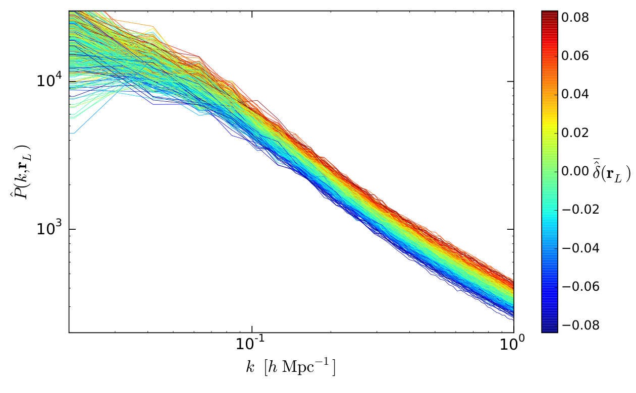
Figure 4.1 shows the position-dependent power spectrum measured from 512 subvolumes with in one realization at . The color represents of each subvolume. The positive correlation between the subvolume power spectra and is obvious. The response of the position-dependent power spectrum to the long-wavelength density fluctuation is clearly measurable at high significance in the simulations.
We measure the integrated bispectrum through
| (4.12) |
where and are measured in the subvolume. Further, motivated by eq. (4.4), we normalize the integrated bispectrum by the mean power spectrum in the subvolumes,
| (4.13) |
and the variance of the mean density fluctuation in the subvolumes,
| (4.14) |
Note that by construction
| (4.15) |
This quantity
| (4.16) |
is the estimator of the normalized integrated bispectrum (eq. (4.8)), and is equal to the linear response function, , given in eq. (4.7) in the limit of .
Figure 4.2 shows the normalized integrated bispectrum, averaged over 160 collisionless -body simulations at different redshifts. For clarity, no error bars are shown in this figure. We have compared the results with a higher-resolution simulation with particles and starting at higher redshift ( compared to for our 160 simulations). For the scales and redshifts shown in figure 4.2, the differences are less than 1%. However, we expect an up to 5% uncertainty in the integrated bispectrum at (less at lower ) due to transients which affect the bispectrum more strongly than the power spectrum [40, 111], as well as other systematics such as mass resolution.
Since the initial conditions are Gaussian, the bispectrum is generated entirely by nonlinear gravitational evolution. We thus measure the effect of a long-wavelength density perturbation on the evolution of small-scale structures. The wiggles visible in each panel of figure 4.2 are due to the BAOs. The BAOs in the right panel are strongly damped because the box size () approaches the BAO scale, and the window function smears the BAO feature [30]. Further, BAO amplitudes are larger at higher redshifts as they are less damped by nonlinear evolution [53]. The broad-band shape of the normalized integrated bispectrum evolves on small scales due to nonlinear evolution, leading to an effective steepening of its slope. We now turn to the theoretical modeling of the results shown in figure 4.2.
4.2 Bispectrum modeling
We use two different approaches to model the integrated bispectrum. In the first approach, we model the bispectrum and compute the integral to obtain the integrated bispectrum. In the second approach, we model the response of the small-scale power spectrum to a long wavelength perturbation directly using the “separate universe” picture. For clarity, we will show the comparison between model prediction and simulations only for the subvolumes (). The agreement with simulations is independent of subvolume size as long as the subvolume size is large enough for to be in the linear regime, and the window function is taken into account.
We first compute the integrated bispectrum by using a model for the bispectrum in eq. (4.3) and perform the eight-dimensional integral. Because of the high dimensionality, we use the Monte Carlo integration routine in GNU Scientific Library to evaluate the angular-averaged integrated bispectrum. In the following, we consider two different models for the matter bispectrum.
4.2.1 Standard perturbation theory
The standard perturbation theory (SPT) [17] gives the tree-level matter bispectrum as
| (4.17) |
where is the linear matter power spectrum, and
| (4.18) |
In order to normalize the integrated bispectrum, we need an expression for the mean subvolume power spectrum . For this we use the linear power spectrum convolved with the window function,
| (4.19) |
while the variance of the mean density fluctuation in the subvolumes is given by eq. (4.5). Both quantities are calculated through Monte Carlo integration.
We compare the normalized integrated bispectrum measured from the simulations with the SPT prediction in figure 4.3 (red lines). The SPT prediction is independent of redshift. This is because the linear power spectra at various redshifts are only different by the wavenumber-independent linear growth factor, . Therefore, the linear growth factor cancels out in the normalized integrated bispectrum. The SPT predictions agree with the simulations relatively well at and , whereas they fail at lower redshifts as well as on smaller scales, where nonlinearities become too strong to be described by SPT. Especially, the BAO amplitudes at are affected: while the SPT predictions are redshift-independent, the simulations show smaller BAO amplitudes at lower redshifts.
The eight-dimensional integral in eq. (4.3) simplifies greatly if we focus on the squeezed-limit bispectrum. In appendix A, we show (note that )
| (4.20) |
for . We can then apply eq. (4.4) and perform all the integrals analytically in the limit of to obtain
| (4.21) |
Comparing this result with eq. (4.7), we find that the linear response of the power spectrum in SPT is given by
| (4.22) |
The green dashed lines in figure 4.3 show the squeezed-limit approximation given in eq. (4.21). While they are different from the full integration (red solid lines) at , for which the squeezed-limit approximation fails and the direct integration is required, they agree well, with the fractional difference being less than 1.5% (1% for ), at , corresponding to a value of . Thus, the squeezed-limit is reached already with good precision for .
Eq. (4.21) does not contain any window function effect apart from that in the variance . While this is a good approximation for the slowly-varying part of the integrated bispectrum, it does not capture the smearing of the BAO features due to the window function. We incorporate this effect by replacing with appropriately convolved forms, , in eq. (4.21). This form is motivated by the separate universe approach discussed in section 4.3, and provides an accurate result as shown in figure 4.3.
4.2.2 Bispectrum fitting formula
The SPT predictions fail on smaller scales as well as at lower redshifts where nonlinearity becomes too strong to be described by SPT. An empirical fitting formula for nonlinear evolution of the matter bispectrum was proposed in [140] and further improved in [64]. In short, the form is the same as the tree-level matter bispectrum, but is replaced by an effective kernel, , which contains nine fitting parameters, , to account for nonlinearity (see eqs. 2.6 and 2.12 in [64] for details). Therefore, we use and compute the integrated bispectrum by performing the eight-dimensional integral numerically with Monte Carlo integration. We use the same values of the best-fit parameters provided in table 2 of [64], which were calibrated by fitting to simulation results between and . In contrast to the SPT formalism that uses the linear power spectrum in eq. (4.17), the fitting formula uses the nonlinear power spectrum, for which we use the mean power spectrum measured from the 160 simulation boxes. For the normalization of the integrated bispectrum, we convolve the nonlinear power spectrum with the subvolume window function as in eq. (4.19). Note that the fitting formula is not specifically designed for the squeezed configuration, but instead was calibrated to a wide range of triangle configurations of the matter bispectrum.
The blue dot-dashed lines in figure 4.3 show the normalized integrated bispectrum computed with , which clearly depends on redshift. At , the modeling and the simulations are in good agreement at . At , although the modeling predicts larger broad-band power of the normalized integrated bispectrum, the BAO amplitudes still agree well with the simulations. This is most obvious for the two BAO peaks at . On the other hand, at , the modeling predicts much larger normalized integrated bispectrum on small scales than measured in the simulations, so that the fitting formula does not perform much better than tree-level perturbation theory at .
4.3 Separate universe approach
In the second approach, we compute the effects of a long-wavelength density fluctuation on the small-scale power spectrum by treating each over- and under dense region as a separate universe with a different background density. This approach thus neglects the finite size of the subvolumes and is valid for wavenumbers which satisfy (specifically, for percent-level accuracy).
The power spectrum in a separate universe with an infinite-wavelength density perturbation, , with respect to the global flat CDM cosmology can be expanded as in eq. (4.6). Through eqs. (4.7)–(4.8), the normalized integrated bispectrum is equal to the linear response of the nonlinear matter power spectrum at wavenumber to :
| (4.23) |
This is not exactly true if the subvolumes for which is measured are not spherical. For example, since the cubic window function is anisotropic, the integrated bispectrum might pick up contributions from the tidal field. However, we have verified that the anisotropy of the cubic window function has a negligible effect, by computing the dipole and quadrupole of the integrated bispectrum through eq. (4.3). The ratios to the monopole are less than on the scales of interest.
A universe with an infinite-wavelength density perturbation with respect to a flat fiducial cosmology is equivalent to a universe with non-zero curvature. This alters the scale factor, Hubble rate, and linear growth as shown in chapter 3, and thus affects the power spectrum. Say this long-wavelength overdensity is
| (4.24) |
where is the background matter density in the fiducial cosmology, is the linear growth factor in the same cosmology, is the background matter density in a slightly curved universe, is a reference time such that , and is the density perturbation at . Note that as in chapter 3, we denote the quantities in the modified (curved) cosmology with a tilde.
In eq. (4.24) and in the following of this section, we assume that is small and evolves linearly. This is justified because here we consider the subvolume to be , and so . One can also see this in figure 4.1: in 512 subvolumes with of one realization at . Therefore, we shall consider the effect on the power spectrum only to the linear order in , and drop for .
With this assumption, the scale factor in the modified cosmology is given by
| (4.25) |
Since the physical coordinates are the same in two cosmologies, this implies that the comoving coordinates of the two cosmologies are related by
| (4.26) |
What we want is to compare the observables between the fiducial and modified cosmologies, so the quantities computed in the comoving coordinates of the modified cosmology have to be mapped to that with respect to the comoving coordinates of the fiducial cosmology. Specifically, in order to match to the comoving coordinates of the fiducial cosmology, we transform the comoving coordinates in the modified cosmology as
| (4.27) |
where c is a constant at a given time. This assures .
Let us now consider how the transform in the coordinates affects the two-point statistics. Since the correlation function is a dimensionless scalar quantity, in the new coordinates with the transformation of (for , 1, and 2) the correlation function must be
| (4.28) |
The power spectrum is then transformed as
| (4.29) |
where we define . This makes sense because and so (see also appendix A of [123]).
Inserting through eq. (4.27), we have the change in power spectrum up to the linear order of as
| (4.30) |
Eq. (4.30) is also known as the “dilation” effect in [97, 98], which is the consequence that the presence of the long-wavelength overdensity perturbation slows down the local expansion rate.
Another effect arises due to the change in the “reference density”. That is, the background density in two cosmologies are related by , and since power spectrum is proportional to density squared, in the overdense universe the power spectrum at the linear order of becomes
| (4.31) |
Combining the effects of dilation and the reference density, and using the scale factor instead of time, the power spectrum in the presence of is given by
| (4.32) |
Note that this expression is only valid to linear order in .
Both and are measured in a finite volume, described by the window function . In order to take this into account, eq. (4.32) is convolved by the window function. Note that we take the convolution after applying the derivative , rather than taking the derivative of the convolved power spectrum. This is because the window function is fixed in terms of observed coordinates (in the fiducial cosmology), i.e., it is not subject to the rescaling of eq. (4.26). Taking the slope of the convolved power spectrum would correspond to a window function defined in the “local” curved cosmology.
4.3.1 Linear power spectrum
For the linear power spectrum, , we have
| (4.33) |
As shown in section 3.2.2 (see also appendix D of [11]), the linear growth factor is changed following
| (4.34) |
where is the growth factor in the fiducial cosmology. The prefactor is only strictly valid for an Einstein-de Sitter cosmology; however, the cosmology dependence is very mild. The fractional difference of between CDM cosmology and Einstein-de Sitter universe at is at the 0.1% level.
4.3.2 SPT 1-loop power spectrum
Expanding matter density fluctuations to third order, one obtains the so-called “SPT 1-loop power spectrum” given by , where [17]
| (4.36) | ||||
Both and are proportional to . Modifying the growth factor as described in section 4.3.1, we obtain the linear response function of the SPT 1-loop power spectrum as
| (4.37) |
Note that this can easily be generalized to loops in perturbation theory by using that . We include the window function effect by computing .
Figure 4.4 compares the linear theory and the SPT 1-loop predictions with the -body simulation results. The SPT 1-loop prediction captures the damping of BAOs due to nonlinear evolution, and agrees well with the simulation results at , 2, and 3. This is expected from the excellent performance of the 1-loop matter power spectrum at high redshifts as demonstrated by [77]. The agreement degrades rapidly at , also as expected. Note that comparing and 3, the 1-loop prediction seems to agree better with the measurements at . However, as mentioned in section 4.1, transients and other systematics might have an impact of up to 5% on the measurements at , which is larger than the difference shown in the top left panel of figure 4.4.
4.3.3 halofit and Coyote emulator
We now apply the separate universe approach to simulation-calibrated fitting formulae for the nonlinear matter power spectrum, specifically the halofit prescription [152] and the Coyote emulator [70]. These prescriptions yield for a given set of cosmological parameters, so that eq. (4.32) can be immediately applied. However, the Coyote emulator does not provide predictions for curved cosmologies, and we hence adopt a simpler approach here.
In case of the linear power spectrum, the effect of the modified cosmology enters only through the modified growth factor given in eq. (4.34). Correspondingly, we can approximate the effect on the nonlinear power spectrum by a change in the value of the power spectrum normalization at redshift zero,
| (4.38) |
where we have used the Einstein-de Sitter prediction. Therefore, the nonlinear power spectrum response becomes
| (4.39) |
The results of applying eq. (4.39) to halofit (red solid) and the Coyote emulator (green dot-dashed) are shown in figure 4.5. In terms of broad-band power, the halofit prediction provides a good match. However, the predicted BAO amplitude are larger than the measurement, especially at low redshift at . Also, while the BAO phases of halofit follow the SPT prediction, there are some differences with respect to the measurement of the -body simulations due to the nonlinear evolution. The Coyote emulator performs to better than % over the entire range of scales and redshifts. It slightly underpredicts the small-scale power at for . For redshifts and on the scales considered, the 1-loop predictions are of comparable accuracy to the Coyote emulator, while the latter provides a better fit at lower redshifts. Finally, note also our previous caveat regarding transients at the end of section 4.3.2.
4.3.4 Halo model
In the halo model (see [35] for a review), all matter is assumed to be contained within halos with a certain distribution of mass given by the mass function, and a certain density profile. Along with the clustering properties of the halos, these quantities then determine the statistics of the matter density field on all scales including the nonlinear regime. -point functions can be conveniently decomposed into one- through -halo pieces. In the following, we will follow the most common halo model approach and assume a linear local bias of the halos.
Adopting the notation of [157], the halo model power spectrum, , is given by
| (4.40) |
where
| (4.41) |
and is the mass function (comoving number density per interval in log mass), is the halo mass, is the -th order local bias parameter, and is the dimensionless Fourier transform of the halo density profile, for which we use the NFW profile [118]. We normalize so that . The notation given in eq. (4.41) assumes . depends on through the scale radius , which in turn is given through the mass-concentration relation. All functions of in eq. (4.41) are also functions of although we have not shown this for clarity. In the following, we adopt the Sheth-Tormen mass function [149] with the corresponding peak-background split bias, and the mass-concentration relation of [24]. The exact choice of the latter has negligible impact on the mildly nonlinear scales, but does not affect the conclusion.
We now derive how the power spectrum given in eq. (4.40) responds to an infinitely long-wavelength density perturbation , as was done for the halofit and Coyote emulator approaches. For this, we consider the one-halo and two-halo terms separately. The key physical assumption we make is that halo profiles in physical coordinates are unchanged by the long-wavelength density perturbation. That is, halos at a given mass in the presence of have the same scale radius and scale density as in the fiducial cosmology. This assumption, which is related to the stable clustering hypothesis, can be tested independently with simulations, but we shall leave it for future work. Given this assumption, the density perturbation then mainly affects the linear power spectrum, which determines the halo-halo clustering (two-halo term), and the abundance of halos at a given mass.
We begin with the two-halo term. The response of the linear power spectrum is given by eq. (4.35). The expression for the two-halo term in eq. (4.40) is simply the convolution (in configuration space) of the halo correlation function in the linear bias model with the halo density profiles. By assumption, the density profiles do not change, hence only changes through the bias and the mass function . The bias quantifies the -th order response of the mass function to an infinite-wavelength density perturbation [115, 137]:
| (4.42) |
We then have
| (4.43) |
Thus,
| (4.44) |
In the large-scale limit, , this vanishes by way of the halo model consistency relation
| (4.45) |
For finite however, eq. (4.44) does not vanish. Thus, the linear response function of the two-halo term becomes
| (4.46) |
Note that we recover the tree-level result given in eq. (4.35) in the large-scale limit. Strictly speaking, this expression is not consistent, since the term implies a non-zero while in eq. (4.40) we have assumed a pure linear bias. Of course, if we allowed for in eq. (4.40), we would obtain a contribution from in eq. (4.46), and so on. This reflects the fact that the halo model itself cannot be made entirely self-consistent. Note that in eq. (4.46) the slope is taken from the linear, not two-halo power spectrum. This is a consequence of our assumption that halo profiles do not change due to ; in other words, having would imply that the profiles do change (in the sense that they are fixed in comoving, rather than physical coordinates).
We now turn to the one-halo term. Given our assumption about density profiles, this term is much simpler. The only effect is the change in the mass function, which through eq. (4.42) (for ) yields
| (4.47) |
We thus obtain
| (4.48) |
Putting everything together, we obtain
| (4.49) |
The prediction of eq. (4.49) is shown as the blue dashed lines in figure 4.5. The amplitude and broad-band shape agree with the simulations well. The main discrepancy in the halo model prediction is the insufficient damping of the BAO wiggles.
An alternative approach to derive the halo model prediction for is to use higher -point functions [84, 97], which are decomposed into one-, halo terms. We now compare eq. (4.49) with the results of [97], which were derived from the halo model four-point function in the collapsed limit. Note that the squeezed limit is assumed in both approaches. Their eq. (27) is
| (4.50) |
There are two differences to eq. (4.49): the term is absent, and the slope is taken from from rather than . The term is absent in eq. (4.50) as by assumption was taken to be zero in the four-point function of [97]; as discussed above, its inclusion is somewhat ambiguous given the lack of self-consistency of the halo model approach. The different power spectrum slopes are due to the different sources of this term in the two derivations. In our case, the assumption of unchanged halo profiles dictates the form of eq. (4.49). In the derivation of eq. (4.50), the slope originates from the integral over the kernel in the three-halo term, which proceeds as described in appendix A but involves instead of . Note however that the numerical difference between eq. (4.50) and eq. (4.49) is only at the percent level.
4.4 Dependence on cosmological parameters
Both the matter power spectrum and (integrated) bispectrum depend on the cosmological parameters such as . However, the normalized integrated bispectrum is much less sensitive to cosmology as the leading cosmology dependence is taken out by the normalizing denominator.
Eq. (4.37) is useful for understanding the dependence of the response function of the power spectrum (and thus the normalized integrated bispectrum) on cosmological parameters. The second term depends on the local spectral index of the matter power spectrum, , which depends on the initial power spectrum tilt, , and the matter and radiation densities which change the redshift of matter-radiation equality as well as the BAO scale. It also depends on the shape of BAO wiggles, and increasing the amplitude of the matter power spectrum () leads to a stronger damping of the BAO feature. Increasing further increases the last term, which is proportional to .
Figure 4.6 shows the linear response functions, computed from the SPT 1-loop power spectrum (eq. (4.37)) at when varying cosmological parameters by . The effects on the response functions are at the percent level or less, illustrating the weak cosmology dependence of this observable. On the scales considered, the shift in the BAO scale when varying leads to the relatively largest effect. We expect that the sensitivity to changes in will be higher on smaller, more nonlinear scales.
4.5 Fisher matrix calculation
Now that we understand the behavior of the integrated bispectrum, how does it compare with the full bispectrum in terms of measuring the cosmological parameters, particularly the primordial non-Gaussianity? In this section, we perform the Fisher matrix calculation (see e.g. [160] for a review) for both the full bispectrum analysis and the integrated bispectrum technique, and compare the performances between the two methods. We shall use the simplest primordial non-Gaussianity model as discussed in section 2.1.4, i.e.
| (4.51) |
The Fisher matrix of the reduced bispectrum is given by
| (4.52) |
where have to form a triangle, are the parameters we want to constrain, and is the variance of the reduced bispectrum estimator. Similarly, the Fisher matrix of the integrated bispectrum can be written as
| (4.53) |
Here, we ignore off-diagonal elements of the covariance matrix of or . In general, nonlinear evolution generates non-vanishing covariances. This is, however, justified at high redshift () as we show in the right panel of figure B.1.
The variance of the estimator for the integrated bispectrum is computed in appendix B. The variance of the estimator for the bispectrum is computed [144]
| (4.54) |
where , 2, 1 for equilateral, isosceles, and general triangles, respectively (we set to be the fundamental frequency). Similar to the integrated bispectrum, we assume that the variance of the reduced bispectrum is dominated by the numerators, so
| (4.55) |
Since galaxies are observed in redshift space, we model the redshift-space distortions by the simple Kaiser factor, and , where the subscripts and denote the real- and redshift-space quantities, and
| (4.56) |
with being the growth rate. The derivatives of and with respect to thus contain the contributions from and . The variances of the redshift-space reduced bispectrum and the normalized integrated bispectrum with the Poisson shot noise are then given by
| (4.57) |
where , , and .
Figure 4.7 shows the two-dimensional joint 95% C.L. constraints on galaxy bias and primordial non-Gaussianity for BOSS [4] (left) and HETDEX [71] (right). The survey parameters and the fiducial cosmological parameters are shown in the top-right of each panel. The blue dashed line is the full bispectrum analysis with being the fundamental frequency of the entire survey ; the green solid line is the full bispectrum analysis with being the fundamental frequency of the largest subvolume for the integrated bispectrum (); the red dot-dashed line is the integrated bispectrum with six sizes of subvolumes from to (with an increment of ) with being the fundamental frequency of the corresponding subvolumes.
One finds that as long as is set to be the fundamental frequency of the largest subvolume, the integrated bispectrum technique gives the similar constraint on compared to the full bispectrum analysis.22 2 Note that the numerical results are sensitive to the choices of and because we count the Fourier modes in this range. For different lines, although is set to be the same, in practice we stop counting Fourier modes if . Therefore they have different “true” , and the contour area would be affected, especially the green solid lines seem to have slightly worse constraints on compared to the red dot-dashed lines. Here, however, what we are interested in is the general properties between different methods, so we should neglect the effect due to different . On the other hand, the integrated bispectrum has poor constraints on and compared to the full bispectrum analysis. In particular, in the top-left panel the signal of integrated bispectrum has a strong degeneracy between and . This is somewhat expected because in figure 2.1 one finds that not only the black solid and black dashed lines have similar scale dependences in a given subvolume, but in different subvolumes they all have similar contribution, unlike the bispectrum of the primordial non-Gaussianity. This thus makes it difficult to break the degeneracy between and using the integrated bispectrum.
We also find that while the full bispectrum analysis and the integrated bispectrum technique give similar constraints on , the number of counted Fourier modes differ dramatically. For example, for the BOSS parameter, the full bispectrum analysis with counts 7113 configurations of triangles, whereas the integrated bispectrum technique counts only 54 Fourier modes. Even if is set to be for the full bispectrum analysis, there are still 6730 configurations of triangles. This is a big advantage for the integrated bispectrum technique because estimating the covariance matrix from mock catalogs would require a large number of realizations, which will be difficult (but not impossible) to obtain for the full bispectrum. This difference in the number of counted Fourier modes also explains why the full bispectrum analysis has much better constraints on and . However, many of the triangles do not contain much more information on , so if one is interested in measuring , the integrated bispectrum technique provides an easier approach and captures most of the information.
4.6 Discussion and conclusion
In this chapter, we have demonstrated a novel method to measure the squeezed-limit bispectrum. By measuring the correlation between the mean density fluctuation and the position-dependent power spectrum, we obtain a measurement of an integral of the bispectrum (integrated bispectrum) without having to actually measure three-point correlations in the data. The integrated bispectrum is dominated by the squeezed-limit bispectrum, which is much easier to model than the full bispectrum for all configurations. This is evidenced by figure 4.4 and figure 4.5, where we show model predictions accurate to a few percent using existing techniques and without tuning any parameters.
A further, key advantage of this new observable is that both the mean density fluctuation and the power spectrum are significantly easier to measure in actual surveys than the bispectrum in terms of survey selection functions. In particular, the procedures developed for power spectrum estimation can be directly applied to the measurement of the position-dependent power spectrum. Additionally, the position-dependent power spectrum depends on only one wavenumber (at fixed size of the subvolume) rather than the three wavenumbers of the bispectrum. Consequently, the covariance matrix also becomes easier to model.
We have measured the position-dependent power spectrum in 160 collisionless -body simulations with Gaussian initial conditions, and have used two different approaches, bispectrum modeling and the separate universe approach, to model the measurements. All of the approaches work well on large scales, , and at high redshift. On small scales, where nonlinearities become important, the separate universe approach (section 4.3) applied through the Coyote emulator prescription performs best at redshifts , while the SPT 1-loop predictions perform equally well at . Both show agreement to within a few percent up to . Accurate predictions for the position-dependent power spectrum on these and even smaller scales can be obtained by applying the separate universe approach to dedicated small-box -body simulations of curved cosmologies, as described in section 6.2.
The normalized integrated bispectrum is relatively insensitive to changes in cosmological parameters (section 4.4), and we do not expect that it will allow for competitive cosmology constraints. On the other hand, this property can also be an advantage: since this observable can be predicted accurately without requiring a precise knowledge of the cosmology, it can serve as a useful systematics test for example in weak lensing surveys. As an example, consider eq. (4.4) applied to shear measurements. A constant multiplicative bias in the shear estimation contributes a factor on the left hand side of the equation, and a factor on the right hand side. Thus, by comparing the measured normalized integrated bispectrum with the (essentially cosmology-independent) expectation, one can constrain the multiplicative shear bias.
The position-dependent power spectrum can also naturally be applied to the case of spectroscopic galaxy surveys, in which case the nonlinear bias of the observed tracers also contributes to the bispectrum and position-dependent power spectrum. Thus, when applied to halos or galaxies, this observable can serve as an independent probe of the bias parameters and break degeneracies between bias and growth which are present when only considering the halo or galaxy power spectrum. We shall exploit this to measure the nonlinear bias of the BOSS CMASS galaxies in chapter 5.
We finally use the Fisher matrix to show that if multiple sizes of subvolumes are used, the position-dependent power spectrum captures most of the information of the local-type non-Gaussianity contained in the full bispectrum analysis, but for much less Fourier modes. This is a huge advantage for this novel technique as the computational requirement for estimating the covariance matrix is largely alleviated. Consequently, the position-dependent power spectrum provides an easier approach for hunting the primordial non-Gaussianity for future galaxy surveys.
Chapter 5 Measurement of position-dependent correlation function
In this chapter, we measure the position-dependent correlation function and the integrated three-point function from real data, the SDSS-III Baryon Oscillation Spectroscopic Survey Data Release 10 (BOSS DR10) CMASS sample [3, 6].
As introduced in section 2.2, the correlation between the position-dependent correlation function,
| (5.1) |
and the mean overdensity,
| (5.2) |
is the integrated three-point function
| (5.3) |
where is the size of the subvolume. Inspired by the behavior in the squeezed-limit where , we define the normalized integrated three-point function as with being the variance of the fluctuations in . Note that when comparing the model to the measurements, we shall divide the model by , which is given in eq. (2.37), to correct for the boundary effect.
The integrated three-point function is simply the Fourier transform of the integrated bispectrum
| (5.4) |
Therefore, if we do not have the analytical expression for the three-point function, we can first compute the integrated bispectrum and Fourier transform it to obtain the integrated three-point function. One example is the redshift-space integrated three-point function, for which we first evaluate the redshift-space integrated bispectrum with the explicit expression of the SPT redshift-space bispectrum given in appendix A.2, and then apply eq. (5.4). We also show that the precision of this operation (nine-dimensional integral in total) is within 2% on the scales of interest (, which we will justify in section 5.1.3).
This chapter is organized as follows. In section 5.1 and section 5.2, we measure the position-dependent correlation function from PTHalos mock catalogs [143, 104, 103] and the BOSS DR10 CMASS sample, respectively. The cosmological interpretation of the measurement is in section 5.3. We conclude in section 5.4.
5.1 Measurement of PTHalos mock catalogs
We first apply the position-dependent correlation function technique to the 600 PTHalos mock galaxy catalogs of the BOSS DR10 CMASS sample in the North Galactic Cap (NGC). From now on, we refer to the real and mock BOSS DR10 CMASS samples as the “observations” and “mocks”, respectively.
We use the redshift range of , and each realization of mocks contains roughly 400,000 galaxies. We convert the positions of galaxies in RA, DEC, and redshift to comoving distances using the cosmological parameters of the mocks. The mocks have the same observational conditions as the observations, and we correct the observational systematics by weighting each galaxy differently. Specifically, we upweight a galaxy if its nearest neighbor has a redshift failure () or a missing redshift due to a close pair (). We further apply weights to correct for the correlation between the number density of the observed galaxies and stellar density () and seeing (). We apply the same weights as done in the analyses of the BOSS collaboration, namely FKP weighting, [56], where , and and “” are the expected galaxy number density and the survey completeness, respectively, provided in the catalogs. Therefore, each galaxy is weighted by .
In this section, we present measurements from mocks in real space in section 5.1.3 and redshift space in section 5.1.4. The application to the CMASS DR10 sample is the subject of section 5.2.
5.1.1 Dividing the subvolumes
We use SDSSPix11 1 SDSSPix: http://dls.physics.ucdavis.edu/~scranton/SDSSPix to pixelize the DR10 survey area. In short, at the lowest resolution (res=1) SDSSPix divides the sphere equally into longitudinal slices across the hemisphere (at equator each slice is 10 degrees wide), and each slice is divided into pieces along constant latitudes with equal area. Thus, for res=1 there are pixels. In general the total number of pixels is , and in this chapter we shall set res=1024. After the pixelization, the object (a galaxy or a random sample) has the pixel number .
We use two different subvolume sizes. To cut the irregular survey volume into subvolumes with roughly the same size, we first divide the random samples at all redshifts into 10 and 20 slices across longitudes with similar numbers of random samples; we then divide the random samples in each slice into 5 and 10 segments across latitudes with similar numbers of random samples. Figure 5.1 shows the two resolutions of our subvolumes before the redshift cuts. (Note that this resolution is different from the resolution of SDSSPix, which we always set to res=1024.) Each colored pattern extends over the redshift direction. Finally, we divide the two resolutions into three (, 0.5717) and five (, 0.52235, 0.55825, 0.60435) redshift bins.
As a result, there are 150 and 1000 subvolumes for the low and high resolution configurations, respectively. The sizes of the subvolumes are approximately and , respectively22 2 The shapes of the subvolumes are not exactly cubes. For example, for the high resolution, the ratios of square root of the area to the depth, , are roughly 0.78, 1.42, 1.51, 1.28, and 0.71, from the lowest to the highest redshift bins. The results are not sensitive to the exact shape of the subvolumes, as long as the separation of the position-dependent correlation function that we are interested in is sufficiently smaller than , , and .. The fractional differences between the numbers of the random samples in subvolumes for the low and high resolutions are within and , respectively. Since the number of random samples represents the effective volume, all subvolumes at a given resolution have similar effective volumes. We assign galaxies into subvolumes following the division of random samples.


5.1.2 Estimators in the subvolumes
In the subvolume, we measure the mean overdensity with respect to the entire NGC, , and the position-dependent correlation function, . The mean overdensity is estimated by comparing the total weighted galaxies to the expected number density given by the random samples, i.e.,
| (5.5) |
where and are the total weights () of galaxies and random samples in the subvolume, respectively, and is the number of subvolumes.
We use the Landy-Szalay estimator [91] to estimate the position-dependent correlation function as
| (5.6) |
where , , and are the weighted numbers of galaxy-galaxy, galaxy-random, and random-random pairs within the subvolume, respectively, and is the cosine between the line-of-sight vector and the vector connecting galaxy pairs (). The summations such as and denote the sum over all the random samples and galaxies within the subvolume, respectively. The angular average correlation function is then .
Eq. (5.6) estimates the correlation function assuming that the density fluctuation is measured relative to the mean. However, the position-dependent correlation function defined in eq. (5.1) uses the density fluctuation relative to the global mean. These two fluctuations can be related by with . Thus, the position-dependent correlation function, , is related to the Landy-Szalay estimator as
| (5.7) |
To compute the average quantities over all subvolumes, we weight by in the corresponding subvolume. For example, for a given variable in the subvolume, the average over all subvolumes, , is defined by
| (5.8) |
Since the number of random samples in each subvolume represents the effective volume, the average quantities are effective-volume weighted. Eq. (5.8) assures that the mean of the individual subvolume overdensities is zero,
| (5.9) |
We also confirm that from eq. (5.7) agrees with the two-point function of all galaxies in the entire survey, on scales smaller than the subvolume size. With and , we estimate the shot-noise-corrected integrated three-point function in the subvolume of size as
| (5.10) |
where the second term in the parentheses is the shot noise contribution, and and are the expected galaxy number density and the survey completeness, respectively, of the random samples. Similarly, we estimate the shot-noise-corrected variance of the fluctuations in the subvolumes of size as
| (5.11) |
where the second term in the parentheses is the shot noise contribution. We find that the shot noise is subdominant (less than 10%) in both and .
5.1.3 Measurements in real space
Figure 5.2 shows the measurements of the two-point function from the entire survey (top left) and the normalized integrated three-point functions (bottom panels),
| (5.12) |
for the subvolumes of two sizes ( in the bottom-left and in the bottom-right panels). The gray lines show individual realizations, while the dashed lines show the mean.
We now fit models of and to the measurements in . We choose this fitting range because there are less galaxy pairs at larger separations due to the subvolume size, and the nonlinear effect becomes too large for our SPT predictions to be applicable at smaller separations. For the two-point function, we take the Fourier transform of [42]
| (5.13) |
where is the linear bias, is the linear power spectrum, is the mode coupling constant, and
| (5.14) |
Hence, with
| (5.15) |
We use a fixed value of . Varying it has only small effect on the other fitted parameters. For the integrated three-point function, we use the SPT calculation with the boundary effect correction, which is given by
| (5.16) |
where and are computed from eq. (5.3) with eq. (2.40) and eq. (2.42), respectively, and is the variance of the linear power spectrum computed from eq. (2.43), using the subvolume sizes of and and the redshift of . Note that the size of the subvolumes affects the values of . We determine by first measuring using the real-space two-point function of the entire survey, and then find such that assuming the cubic top-hat window function33 3 In principle, the shape of the window function also affects , but we ignore this small effect.. We find that these values ( and ) agree well with the cubic root of the total survey volume divided by the number of subvolumes, to within a few percent.
We fit the models to and of both subvolumes simultaneously by minimizing
| (5.17) |
where is the inverse covariance matrix computed from the 600 mocks, and are the data and the model in the bin, respectively. The models contain three fitting parameters , , and .
The models computed with the mean of the best-fitting parameters of 600 mocks are shown as the black solid lines in figure 5.2. The best-fitting parameters are , , and , where the error bars are 1- standard deviations. The agreement between the models and the mocks is good, with a difference much smaller than the scatter among 600 mocks. Upon scrutinizing, the difference in is larger for larger separations because the fit is dominated by the small separations with smaller error bars. On the other hand, for the agreement is good for two sizes of subvolumes at all scales of interest. This indicates that the SPT calculation is sufficient to capture the three-point function of the mocks in real space.
The data points in figure 5.2 are highly correlated. To quantify the quality of the fit, we compute the -histogram from 600 mocks, and compare it with the -distribution with the corresponding degrees of freedom (d.o.f.). There are 13 fitting points for each measurement ( and two sizes of subvolumes for ) and three fitting parameters, so d.o.f.=36. The top right panel of figure 5.2 shows the -histogram. The dashed line shows the -distribution with d.o.f.=36. The agreement is good, and we conclude that our models well describe both and of the mocks in real space.
Our is in good agreement with the results presented in figure 16 of [62], whereas our is smaller than theirs, which is , by 1.2. This may be due to the difference in the bispectrum models. While we restrict to the local bias model and the tree-level bispectrum, [62] includes a non-local tidal bias [113, 9, 148] and uses more sophisticated bispectrum modeling using the effective kernel [64, 63]. In appendix D, we show that using the effective kernel and the non-local tidal bias in the model increases the value of , but the changes are well within the 1- uncertainties. Also, the differences of the goodness of fit for various models are negligible.
The fitting range as well as the shapes of the bispectrum may also affect the results: the integrated correlation function is sensitive only to the squeezed configurations, whereas [62] includes more equilateral and collapsed triangle configurations. Understanding this difference merits further investigations.
5.1.4 Measurements in redshift space
Figure 5.3 shows the measurements of (top left) and ( in the bottom-left and in the bottom-right panels) of the mocks in redshift space. The gray lines show individual realizations, while the dashed lines show the mean. Similar to the analysis in section 5.1.3, we fit the models in redshift space to the measurements in . In this section, we use General Relativity to compute the growth rate, , which yields . We shall allow to vary when interpreting the measurements in the actual data.
Since there is no baryonic acoustic oscillation feature on the scales we are interested in, we model the redshift-space two-point correlation function as
| (5.18) |
where and are given in eq. (5.15) and
| (5.19) |
is the Kaiser factor with [80]. As we do not include the subdominant term proportional to in the two-point function, it only gives constraint on , which we can then use to break the degeneracy with in the integrated three-point function. We find that this simple modeling yields unbiased and fulfills the demand. We calculate the redshift-space integrated three-point function by first evaluating the integrated bispectrum using SPT at the tree level (the explicit expression of the redshift-space bispectrum is given in appendix A.2), compute its one-dimensional Fourier transform, as eq. (5.4), and then correct for the boundary effect. The of the mocks in redshift space agrees with to percent level. The redshift-space models thus contain, as before in real space, the three fitting parameters, , , and . We then simultaneously fit and of both subvolumes by minimizing eq. (5.17). Figure 5.4 shows the correlation matrix ( in , normalized by ) estimated from the 600 mocks in redshift space. Because we normalize the integrated three-point function by , the covariance between and is negligible. On the other hand, the covariances between and , between , and between for two sizes of subvolumes are significant.
The models computed with the mean of the best-fitting parameters of 600 mocks are shown as the thick solid lines in figure 5.3. The best-fitting parameters are , , and . The agreement between the models and the measurements in redshift space is as good as in real space.
Again, our is in good agreement with the results presented in figure 16 of [62], whereas our is smaller than theirs, which is , but still well within the 1- uncertainty. As noted in section 5.1.3, the adopted models of the bispectrum are different. In appendix D, we show that using the effective and kernels and the non-local tidal bias in the model increases the value of . However, the changes are within the uncertainties, and the goodness of the fit is similar for different models. Thus, in this paper we shall primarily use the SPT at the tree level with local bias for simpler interpretation of the three-point function, but also report the results for the extended models.
5.2 Measurement of the BOSS DR10 CMASS sample
We now present measurements of the position-dependent correlation function from the BOSS DR10 CMASS sample44 4 Catalogs of galaxies and the random samples can be found in http://www.sdss3.org. in NGC. The detailed description of the observations can be found in [3, 6]. Briefly, the sample contains 392,372 galaxies over 4,892 deg2 in the redshift range of , which corresponds to the comoving volume of approximately . We also weight the galaxies by to correct for the observational systematics. We follow section 5.1.1 to divide the observations into subvolumes. However, the observations have their own set of random samples, which are different from the ones of the mocks (the random samples of the mocks have slightly higher and different ), so we adjust the redshift cuts to be , 0.5717 and , 0.52235, 0.55825, 0.60435 for the two resolutions, respectively. The resulting properties of subvolumes of the observations and mocks are similar.
The mocks are constructed to match the two-point function of the observed galaxies, but not for the three-point function. Hence there is no guarantee that the three-point function of mocks agrees with the observations. We can test this using our measurements.
| avg | var | ||
|---|---|---|---|
The measurements of and from the observations are shown as the solid lines in figure 5.5; the measurements of is summarized in table 5.1. The measurements are consistent visually with the mocks within the scatter of the mocks55 5 These measurements of are done for one effective redshift. We compare of the observations and mocks in different redshift bins in appendix E, finding that the observations and mocks are consistent at all redshift bins to within the scatter of the mocks., and we shall quantify the goodness of fit using statistics later.
To quantify statistical significance of the detection of and the goodness of fit, we use the mean of the mocks as the model (instead of the model based on perturbation theory used in section 5.1.4), and fit only the amplitudes of , , and to the observations and the 600 mocks by minimizing eq. (5.17). Specifically, we use as the model, where , , and , with the amplitudes .
| 1- error | 0.12 | 0.03 | 0.04 |
|---|---|---|---|
| best-fit (DR10) | 0.89 | 1.02 | 1.08 |
| corr | 0.34 | 0.09 | 0.36 |
|---|
Table 5.2 summarizes the fitted amplitudes. The 1- uncertainties and the correlations are estimated from the 600 mocks. Since we normalize by , the correlation between and is small. On the other hand, and are correlated significantly because is an integral of the two-point function [eq. (2.43)].
Comparing the BOSS DR10 CMASS sample to the mean of the mocks, we find that is 1- lower, is unbiased (by construction of the mocks), and is 2- higher. The result of for the data is driven by the correlation between different separations of . On the other hand, the result of is driven by the positive correlation between and . While of the data for two subvolumes are larger than that of the mocks but still at the boundary of the variances (see table 5.1), it requires an even higher to minimize when we jointly fit the three amplitudes. The fact that is larger than is also possibly due the contributions to from small separations (including stochasticity at zero separations), where the mocks were not optimized. We find , i.e., a 7.4 detection of the integrated three-point function of the BOSS DR10 CMASS sample.
In order to assess the goodness of fit, we use the distribution of , a histogram of which is shown in the top right panel of figure 5.5. In total there are 41 fitting points (13 fitting points for and two sizes of subvolumes for , and two fitting points for ) with three fitting parameters, so d.o.f.=38. The value of the observations is 49.3, and the probability to exceed this value is more than 10%. Given the fact that the mocks are constructed to match only the two-point function of the observations, this level of agreement for both the two-point and integrated three-point correlation functions is satisfactory.
5.3 Interpretation for the measurement of the integrated three-point function
What can we learn from the measured ? In section 5.1.4, we show that the prediction for based on SPT at the tree-level in redshift space provides an adequate fit to the mocks to within the scatter of the mocks; thus, we can use this prediction to infer cosmology from . Note that any unmodeled effects in the integrated three-point function such as nonlinearities of the matter density, nonlocal bias parameters, and redshift-space distortions beyond the Kaiser factor, will tend to bias our measurement of cosmological parameters based on . We will discuss caveats at the end of this section.
Since the linear two-point and the tree-level three-point functions are proportional to and , respectively, and is proportional to , the scaling of the redshift-space correlation functions is
| (5.20) |
where “fid” denotes the quantities computed with the fiducial value of . Note that is proportional to because it is an integral of two linear power spectra (see eq. (5.14)). Since dominates the signal, the parameter combinations and are degenerate in the two-point function. That is, the amplitude of the two-point function measures only . This degeneracy can be lifted by including the quadrupole of the two-point function in redshift space. See [130, 164, 131, 19] for the latest measurements using the BOSS DR11 sample.
As for the three-point function, figure 2.2 shows that the and terms are comparable for . This means that, at the three-point function level, the nonlinear bias appears in the leading order, so the amplitude of the three-point function measures a linear combination of and . This provides a wonderful opportunity to determine . The challenge is to break the degeneracy between , , , and . For this purpose, we combine our results with the two-point function in redshift space and the weak lensing measurements of BOSS galaxies. We take the constraints on and from table 2 of [130]. To further break the degeneracy between , , and , we take the constraint on from [114, 117], where they jointly analyze the clustering and the galaxy-galaxy lensing using the BOSS DR11 CMASS sample and the shape catalog from Canada France Hawaii Telescope Legacy Survey.
We assume Gaussian priors on , , and with the known covariance between and . The cross-correlation coefficient between and is , as shown in figure 6 of [130]. We then run the Markov Chain Monte Carlo with the Metropolis-Hastings algorithm to fit he model eq. (5.20) to the observed . We find , and the results for the extended models are summarized in table 5.3.
| baseline | eff kernel | tidal bias | both | |
|---|---|---|---|---|
The value of we find is lower than the mean of the mocks, . The difference is mainly due to two reasons. First, the amplitude of the integrated three-point function of the observations is lower than that of the mocks by 10% (). Second, the priors from the correlation function and lensing constraint to be close to 2.18, which is larger than that of the mocks, . Thus, it requires a smaller to fit the three-point function. The argument is similar for the extended models. Note, however, that the nonlinear bias of the data is still statistically consistent with the mocks.
Let us conclude this section by listing three caveats regarding our cosmological interpretation of the measured integrated three-point function.
- 1.
The models we use, eq. (5.20), are based on tree-level perturbation theory, the lowest order redshift-space distortion treatment, as well as on the local bias parametrization. While this simple model describes the mocks well, as shown in section 5.1.3 and 5.1.4, we discuss in appendix D that using the effective and and the non-local tidal bias brings closer to that of [62]. We, however, find similar goodness of fit for various models, and thus we cannot distinguish between these models.
- 2.
Covariances between the integrated three-point function, monopole and quadrupole two-point function, and weak lensing signals are ignored. This can and should be improved by performing a joint fit to all the observables.
- 3.
The cosmology is fixed throughout the analysis, except for and . In principle, marginalizing over the cosmological parameters is necessary to obtain self-consistent results, although the normalized integrated three-point function is not sensitive to cosmological parameters such as as shown in figure 4.6.
These caveats need to be addressed in the future work.
5.4 Discussion and conclusion
In this chapter, we have reported on the first measurement of the three-point function with the position-dependent correlation function from the SDSS-III BOSS DR10 CMASS sample. The correlation between the position-dependent correlation function measured within subvolumes and the mean overdensities of those subvolumes is robustly detected at 7.4.
Both the position-dependent correlation function and the mean overdensity are easier to measure than the three-point function. The computational expense for the two-point function is much cheaper than the three-point function estimator using the triplet-counting method. In addition, for a fixed size of the subvolume, the integrated three-point function depends only on one variable (i.e., separation), unlike the full three-point function which depends on three separations. This property allows for a useful compression of information in the three-point function in the squeezed configurations, and makes physical sense because the integrated three-point function measures how the small-scale two-point function, which depends only on the separation, responds to a long-wavelength fluctuation, as introduced in chapter 4. As there are only a small number of measurement bins, the covariance matrix of the integrated three-point function is easier to estimate than that of the full three-point function from a realistic number of mocks. We have demonstrated this advantage in this chapter.
Of course, since this technique measures the three-point function with one long-wavelength mode (mean overdensity in the subvolumes) and two relatively small-wavelength modes (position-dependent correlation function), it is not very sensitive to the three-point function of other configurations, which were explored in [62].
We have used the mock galaxy catalogs, which are constructed to match the two-point function of the SDSS-III BOSS DR10 CMASS sample in redshift space, to validate our method and theoretical model. We show that in both real and redshift space, the integrated three-point function of the mocks can be well described by the tree-level SPT model. However, the nonlinear bias which we obtain from the mocks is higher than that reported in [62]. This is possibly due to the differences in the scales and configurations of the three-point function used for the analyses. As discussed in section 5.3, any unmodeled nonlinear effects in the redshift-space integrated three-point function of CMASS galaxies will tend to bias , and will bias this parameter differently than the measurement of [62].
Taking the mean of the mocks as the model, and treating the amplitudes of two- and three-point functions as free parameters, we find the best-fit amplitudes of , , and of the CMASS sample. With respect to the mean of the mocks, the observations show a somewhat smaller () and larger , while the ensemble two-point function matches the mocks. Given that the mocks are generated to match specifically the two-point function of the BOSS DR10 CMASS sample within a certain range of separations, the level of agreement between the observations and mocks is satisfactory.
Finally, by combining the integrated three-point function and the constraints from the anisotropic clustering ( and in [130]) and from the weak lensing measurements ( in [117]), we break the degeneracy between , , , and . We find for the BOSS DR10 CMASS sample. The caveat of this result is that our model, eq. (5.20), relies on a rather simple model in redshift space as well as on the local bias parametrization. We leave the extension of the model to improved bias and redshift-space distortion modeling (especially in light of the comparison with the results in [62]) for future work.
In summary, we have demonstrated that the integrated three-point function is a new observable which can be measured straightforwardly from galaxy surveys using basically the existing and routinely applied machinery to compute the two-point function, and has the potential to yield a useful constraint on the quadratic nonlinear bias parameter. Moreover, since the integrated three-point function is most sensitive to the bispectrum in the squeezed configurations, it is sensitive to primordial non-Gaussianity of the local type (see section 2.1.4 and section 4.5 for more details), thereby offering a probe of the physics of inflation. We plan to extend this work to search for the signature of primordial non-Gaussianity in the full BOSS galaxy sample.
Chapter 6 The angle-averaged squeezed limit of nonlinear matter -point functions and separate universe simulations
In the previous chapters, we have introduced the position-dependent two-point statistics and shown the measurements from -body simulations and observations. In this chapter, we shall generalize the study to the angle-averaged squeezed limit of nonlinear matter -point functions, and demonstrate how to use the “separate universe simulations” to address this issue. Specifically, we consider the case of the squeezed limit such that there is a hierarchy between two large wavenumbers and , and small wavenumbers . The configuration is sketched in figure 6.1.
The squeezed limit of matter -point functions has been the subject of a large body of work in the context of the so-called “consistency relations” for the large-scale structure [85, 127, 39, 83, 166, 165, 84, 38, 37, 120, 15, 73, 121]. The contributions to -point functions in the squeezed limit are ordered by the ratio of wavenumbers , which is assumed to be much less than one. The lowest order contributions, up when the -point function is written in terms of the overdensity , are fixed by the requirement that a uniform potential perturbation as well as a uniform velocity (boost) do not lead to any locally observable effect on the density field, as demanded by the equivalence principle [85, 127, 166, 44]. They are also referred to as “kinematic contributions”.
The next order contribution, , is the lowest order at which a physical coupling of long- and short-wavelength modes happens. More precisely, the contributions at this order correspond to the impact of a uniform long-wavelength density or tidal perturbation. When considering equal-time -point functions and subhorizon perturbations , the kinematic contributions disappear, and the physical contributions are the leading contribution to the -point function in the squeezed limit.
In this chapter, we disregard tidal fields, which leads us to first angle-average over the small momenta (wavenumbers) in the -point function. Specifically, we consider defined through
| (6.1) |
where are unit vectors and denotes the nonlinear connected matter -point function with the momentum constraint dropped. Note that the momentum constraint fixes in terms of and . We now let go to zero, and normalize the result by the nonlinear power spectrum and the linear power spectra to obtain a dimensionless quantity:
| (6.2) |
Note that in this limit, spatial homogeneity enforces , so that (for statistically isotropic initial conditions) the right-hand-sight of eq. (6.2) depends only on .
In appendix F (see also [165]), we show that correspond exactly to the power spectrum response functions, which quantify the change in the nonlinear matter power spectrum to an infinite-wavelength density perturbation. These response functions are defined as the coefficients of the expansion of the power spectrum in the linearly extrapolated initial overdensity :
| (6.3) |
where is the nonlinear matter power spectrum at time in the presence of a homogeneous (infinite-wavelength) density perturbation, and is the linear growth factor normalized to unity today. We have set by definition. Thus, by measuring , we measure the angle-averaged squeezed limit (eq. (6.2)) of the nonlinear matter -point function. For , the response describes the angle-averaged squeezed-limit bispectrum, as discussed in chapter 2 and chapter 4.
Independently of the derivation of eqs. (6.2)–(6.3), we also present accurate measurements of for using -body simulations which do not rely on approximations in section 6.2. Specifically, we resort to -body simulations with an external homogeneous overdensity imposed via the separate universe approach described in chapter 3. A flat FLRW universe with a homogeneous overdensity is exactly equivalent to a different, curved FLRW universe, so that -body simulations in this modified cosmology provide, in principle, the exact result for the response functions . This in turn corresponds to the exact (in the limit of infinite volume and resolution) measurement of the squeezed-limit -point function (eq. (6.2)). The measurements of are presented in [97]. We shall extend to and 3.
Many semi-analytical approaches to nonlinear large-scale structure assume that nonlinear matter statistics can be described as a unique function of the linear matter power spectrum, i.e. the power spectrum of initial fluctuations linearly extrapolated to a given time. In the context of consistency relations, this approximation has been studied in e.g. [165, 84]. This ansatz is motivated by the fact that in Einstein-de Sitter (flat matter-dominated universe), and to a very good approximation in CDM, the perturbation theory predictions factorize into powers of the linear growth factor and convolutions of products of the initial matter power spectra and time-independent functions. Another way to phrase this ansatz is that nonlinear large-scale structure only depends on the normalization of the fluctuations at a given time, and not on the growth history.
In the context of squeezed-limit -point functions, this ansatz can be tested quantitatively by comparing the outputs of separate universe simulations at a given time with simulations in which the initial amplitude of fluctuations is rescaled to match the linear power spectrum at the same time. The difference between these “rescaled initial amplitude” simulations and the separate universe simulations corresponds to the error made in the ansatz of assuming that the linear power spectrum at a given time uniquely describes nonlinear large-scale structure at the same time. For , it is studied in [98] and found that the two simulations differ in the nonlinear regime. A closely related test using the matter bispectrum is shown in [120]. We shall study this comparison in more detail and for and 3 in section 6.4.
This chapter is organized as follows. In section 6.1, we develop semi-analytic predictions for the power spectrum response. In section 6.2, we describe the methodology of performing the separate universe simulations. In section 6.3, we compare the measurements from -body simulations to the semi-analytic predictions. In section 6.4, we compare the rescaled simulations to the separate universe simulations. We conclude in section 6.5.
6.1 Power spectrum response
We define the -th order response function of the power spectrum as the -th derivative of the power spectrum with respect to the linearly extrapolated (or Lagrangian) overdensity , normalized by the power spectrum. The definition, consistent with eq. (6.3), is
| (6.4) |
where . In the following, we will frequently suppress the time argument for clarity. Analogously, one can define the power spectrum response functions with respect to the fully evolved (or Eulerian) nonlinear overdensity . Since we can expand the nonlinear overdensity in powers of with known coefficients via the spherical collapse (see chapter 3), the -th order Eulerian response function is given by a sum of with . Motivated by the relation eq. (6.2), we mainly consider the Lagrangian response functions. In the remainder of this section, we develop semi-analytic models for the response functions based on the separate universe picture.
6.1.1 Separate universe picture
The idea of absorbing an infinitely-wavelength overdensity perturbation into the background modified (curved) cosmology is extensively discussed in chapter 3, and the response of the power spectrum to the overdensity is also discussed in chapter 4 (but restricted to the linear order). In this section, we shall first summarize results, and generalize the study to higher order response, i.e. .
Because of the overdensity, the expansion slows down, and the overdense region behaves as a universe with positive curvature. The scale factor in the modified cosmology can be written as
| (6.5) |
where the quantities in the modified cosmology are denoted with a tilde. Since the physical distance is the same in both cosmologies, eq. (6.5) implies the change of the comving distance to be
| (6.6) |
Furthermore, due to mass conservation, the fractional difference in the scale factor is related to the overdensity by
| (6.7) |
Using the separate universe picture, we consider the matter power spectrum in this patch just as that of a region with no homogeneous overdensity but properly modified cosmology. The modification of the cosmology is such that the shape of the linear power spectrum is unchanged, since the ratio of photon, baryon, and cold dark matter densities is unmodified; moreover, the transfer function parameters are unchanged: and . Thus, only the growth of structure is affected.
The power spectrum that enters in the response given by eq. (6.4) is defined with respect to the background density and comoving coordinates of the fiducial cosmology. Hence, the power spectrum calculated for the modified cosmology has to be mapped to that with respect to the background density and comoving coordinates of the fiducial cosmology. As discussed in chapter 4, this mapping yields the “reference density” and “dilation” contributions to the response. These can be calculated exactly at any scale to any given order given the nonlinear matter power spectrum in the fiducial cosmology. That is, we do not need to run -body simulations to calculate these effects. They are thus merely “projection effects”, unlike the effect of the modified cosmology on the growth of structure, which requires simulations in order to provide an accurate estimate.
Let us denote the power spectrum for the modified cosmology as . Then, the reference density effect simply rescales the power spectrum as,
| (6.8) |
where the argument of is not modified. The dilation effect due to the change in the coordinates given by eq. (6.6) implies and changes the power spectrum by (see chapter 4 for detailed derivation)
| (6.9) |
Putting the two together and using eq. (6.7) yields
| (6.10) |
where all quantities are evaluated at some fixed time . Note that one prefactor of cancels, since the effect of the increased density is partially canceled by the corresponding decrease in physical volume. As derived in chapter 3, for an Einstein de-Sitter fiducial universe (and to high accuracy in CDM) and have series solutions of the form
| (6.11) |
where is the fiducial growth factor normalized to one at the epoch to which we extrapolate . Note that the values of and are given in eq. (3.35) and eq. (3.36), respectively.
The third contribution to comes from the effect of the modified cosmology on the growth of structure, which as mentioned above is the physical contribution which requires -body simulations for an accurate measurement. We thus define a set of growth-only response functions which isolate the nontrivial effect of the long-wavelength perturbation on the growth of small-scale structure,
| (6.12) |
That is, are defined as without the contributions from the reference density and dilation given by eq. (6.10). This definition is an extension of the similar decomposition for shown in [147, 84, 15, 98]. Thus, the formula for the power spectrum (with respect to global coordinates) in the presence of a long-wavelength overdensity is given by
| (6.13) |
Clearly, by the Leibniz rule, at any given order the total or “full” response , eq. (6.4), is composed of the functions and the numbers with , where the multiply derivatives of and with respect to (up to the derivative). Specifically, the first three full response functions are given by
| (6.14) | ||||
| (6.15) | ||||
| (6.16) |
where the primes denote derivatives with respect to .
6.1.2 Linear power spectrum predictions
We now evaluate eq. (6.13) for the simplest case, i.e., the response of the linear matter power spectrum. In linear theory, the growth is scale-independent and given by the linear growth factor. Thus, the growth-only response functions are scale-independent and just described by the linear growth factor in the modified cosmology ,
| (6.17) |
As for and , also has the perturbative expansion in powers of as
| (6.18) |
Thus, for an Einstein-de Sitter fiducial universe (and to high accuracy in CDM), the linear response functions are simply constants. Inserting the values of from eq. (3.49), we obtain
| (6.19) |
eq. (6.13) evaluated for the linear matter power spectrum then becomes
| (6.20) |
Inserting the series expansions, we obtain
| (6.21) |
Eq. (6.21) allows for a consistent expansion in . Specifically, is given by the -th order coefficient in this expansion, multiplied by .
6.1.3 Nonlinear power spectrum predictions
Beyond the linear matter power spectrum, the growth coefficients will become scale-dependent functions . Consider now what standard perturbation theory (SPT) predicts. The power spectrum prediction is given by a series
| (6.22) |
where scales as . In an Einstein-de Sitter universe, one can show (e.g., [17]) that the time- and scale-dependence of each order in perturbation theory factorizes, so that one can write
| (6.23) |
where is a convolution of factors of with time-independent coefficients. While eq. (6.23) is only strictly correct in Einstein-de Sitter, it is used very commonly for CDM as well, since departures from the exact result are typically of order 1% or less, and since it simplifies the calculation significantly. Various variants of SPT, such as the renormalized perturbation theory (RPT) [41], share the same property.
Eq. (6.23) allows for a very simple evaluation of the growth-only response: as discussed above, the shape of the linear power spectrum in the modified cosmology is unchanged, and hence can be simply evaluated by replacing the fiducial in eq. (6.23) with the modified one, eq. (6.18). This is equivalent to assuming that the entire late-time cosmology dependence of the nonlinear matter power spectrum enters through the linear growth factor [165, 84, 15]. In section 6.4, we shall test this prescription to all orders in SPT calculations by performing simulations with a rescaled initial power spectrum.
Apart from the SPT calculation, we can also apply this approximation to any prescription that maps a given linear power spectrum to a nonlinear one. In particular, we will show results for halofit [152]. In this case, where the dependence on the linear growth factor is not explicit, we instead compute the derivative with respect to the normalization of the linear power spectrum,
| (6.24) |
which at the redshift considered yields the equivalent change of the linear matter power spectrum. This leads to
| (6.25) |
We use a five-point stencil with a step size of in to compute numerically the derivatives with respect to . In conjunction with the change of the linear growth factor eq. (6.18), this allows us to compute the growth-only response for perturbation theory as well as fitting formulae of the nonlinear matter power spectrum.
6.1.4 Halo model predictions
In section 4.3.4, we have derived the linear response of the power spectrum under the halo model framework, in which all matter is assumed to be contained within halos with a certain distribution of mass (given by the mass function) and density profile. In this section, we shall focus on generalizing the derivation to higher order responses for the halo model approach.
Adopting the notation in section 4.3.4, the halo model powe spectrum, , is given by
| (6.26) |
where
| (6.27) |
and is the mass function (comoving number density per interval in log mass), is the halo mass, is the -th order local bias parameter, and is the dimensionless Fourier transform of the halo density profile, for which we use the NFW profile. One can find more details in section 4.3.4.
To derive how the power spectrum given in eq. (6.26) responds to a homogeneous (infinitely long-wavelength) density perturbation , we consider the one-halo () and two-halo () terms separately. The key physical assumption we make is that halo profiles in physical coordinates are unchanged by . That is, halos at a given mass in the presence of have the same scale radius and scale density as in the fiducial cosmology. We will discuss this assumption later in this section. Given this assumption, the density perturbation then mainly affects the linear power spectrum, which determines the halo-halo clustering (two-halo term), and the abundance of halos at a given mass.
For the two-halo term, as the response of the linear power spectrum is derived in eq. (6.21), the remaining task is to consider the effect on . By the assumption that the density profile does not change in the presence of , only changes through the bias and the mass function . The bias quantifies the -th order response of the mass function to :
| (6.28) |
Thus,
| (6.29) |
Note that in the large-scale limit, , this vanishes for by way of the halo model consistency relation
| (6.30) |
For finite eq. (6.29) does not vanish, we thus have
| (6.31) |
Thus, the two-halo term in the presence of becomes
| (6.32) | ||||
Note that we recover the tree-level result given in eq. (6.21) in the large-scale limit, where only of the third term in eq. (6.32) survives. Note also that in eq. (6.32) the dilation effect only enters in the linear, not 2-halo, power spectrum. This is a consequence of our assumption that halo profiles do not change due to the long-wavelength density perturbation.
For the one-halo term, due to our assumption about density profiles, the only effect is the change in the mass function, which through eq. (6.28) becomes
| (6.33) |
and thus
| (6.34) |
Putting one-halo and two-halo terms together, we obtain
| (6.35) |
The contribution (for ) is numerically much smaller than the other terms (see also the discussion in section 4.3.4). Since it is much smaller than the overall accuracy of the halo model description, we will neglect it in the following. This yields
| (6.36) |
Explicitly, the first and second order full response functions are given by
| (6.37) |
We also derive the growth-only response functions in the halo model approach. Since the halo profiles are assumed fixed in physical coordinates, this means that we need to rescale the halo model terms, , accordingly. Following our discussion in section 6.1.1, we have , where is the comoving wavenumber with respect to the modified cosmology. We then obtain
| (6.38) |
Inserting this into eq. (6.35) and performing a series expansion of in then allows us to derive the growth-only response functions . Note that the NFW profile we assume is uniquely determined by the scale radius for a halo of mass , which enters the coefficients defined in eq. (6.27) in the combination . Thus, it is easily possible to include a dependence of the scale radius , or equivalently the halo concentration, on the long-wavelength density in a similar way. We will leave this for future work.
Quantitatively, the main contribution of the rescaling eq. (6.38) is from the one-halo term , i.e. the term in the last line of eq. (6.36). The rescaling of the other instances of only changes the response at the sub-percent level and we will neglect them in the following. We then obtain for the growth-only contribution to the halo model power spectrum
| (6.39) |
where
| (6.40) |
6.2 Separate universe simulations
To test our semi-analytical models of the power spectrum response to the homogeneous overdensity, particularly for the growth of structure due to the change of the cosmology, we run separate universe simulations and measure the power spectrum response functions directly. In this section, we describe the details for performing the separate universe simulations. We shall first introduce the straightforward modifications, cosmological parameters and the initial conditions, and then the non-trivial choices, comoving or physical coordinates.
For usual -body codes, one needs to specify the cosmological parameters at present time and the output time normally specified by the scale factor. As discussed in chapter 3, in the presence of the overdensity , the cosmological parameters at are modified as
| (6.41) |
For the output time, because we want to compare the simulations at the same physical time, we need to determine the corresponding scale factor in the modified cosmology such that . We can numerically solve the ordinary differential equation of in the modified cosmologies eq. (3.18); alternatively we can numerically evaluate by
| (6.42) |
In order to generate the initial conditions for -body simulations of the modified cosmologies, we need the linear power spectrum at the initial redshift. The initial power spectrum has to be generated for the cosmology with the same amplitude of the primordial scalar curvature perturbation as for the fiducial cosmology. Since the transfer function only involves the physical matter and radiation densities quantified by and so on, it is identical in the modified and fiducial cosmologies. Therefore, the linear power spectra differ only through the difference in the linear growth factor. We use CAMB [96, 95] to compute the power spectrum of the fiducial cosmology at , and rescale it by
| (6.43) |
where is the scale factor for which the initial conditions are generated.11 1 In order to recover the correct linear power spectrum at low redshifts, we compute the growth functions ( and ) without taking radiation into account. This is because -body codes do not include the effect of cosmological radiation. In our procedure, we also neglect the effect of curvature on the transfer function at very low wavenumbers , since terms of similar order are neglected in the Poisson equation used in -body codes. For sub-horizon box sizes these effects are completely negligible. Next, we generate a Gaussian realization of the density field following the initial power spectrum. The positions and velocities of the particles are computed by the second-order Lagrangian perturbation theory [40].
Given a fixed box size for the fiducial cosmology, there are two reasonable choices for the box sizes of the modified cosmologies. Either we match the respective comoving box sizes, i.e. the box size is in units of Mpc comoving, or we choose the box sizes such that their physical sizes coincide with that of the fiducial simulation at one specific output time , i.e. in units of Mpc comoving. The former choice is adequate if we are interested in the power spectrum response functions at the same comoving wavenumber, i.e. without the “dilation” effect. By using the mean density of the separate universe cosmology as the reference density when computing the power spectrum, we are further removing the “reference density” effect and are left with the growth-only response. The results of these simulations are presented in section 6.3.1.
In order to measure the full response functions, we run simulations for which we match the physical box size. We focus on two different output times corresponding to and in the fiducial cosmology. As the physical size can only be matched at one specific time, we have to run a new set of simulations for each output time. The results of these simulations are presented in section 6.3.2.
Finally, we summarize the common features for the separate universe simulations. All simulations are gravity-only simulations and are carried out using the Tree-PM code Gadget-2 [153]. The starting redshift is (), and the particle load for each simulation is . For the fiducial cosmology (), we choose a flat CDM cosmology with cosmological parameters consistent with the current observational constraints: , , , , , and a comoving box size of .
We simulate separate universes corresponding to the linearly-evolved present-day overdensities of , , , , , , , , , and . Then, for the separate universes, the Hubble constant and the curvature fraction vary between : 0.447 to 0.883 and : to 0.372, respectively. The physical densities , , and as well as and the amplitude of the primordial curvature power spectrum remain the same.
6.3 Results of separate universe simulations
For the power spectrum computation, we first estimate the density contrast on a grid using the cloud-in-cell mass assignment scheme, then apply a Fast Fourier transform, and angular average the squared amplitude . The density contrast describes the overdensity with respect to the reference density . When we are interested in the growth-only response function, is equal to the mean density of the separate universe. When we compute the full response function, is equal to the mean density of the fiducial cosmology. Similarly, for the growth-only response, distances are measured using the comoving coordinates of the respective cosmology22 2 Note, however, that the unit of length is always Mpc, where corresponds to the fiducial cosmology., whereas, for the full response, the power spectrum is always measured in comoving coordinates of the fiducial cosmology.
We only report results up to a maximum wavenumber of . A convergence study with simulations with 8 times lower mass resolution shows differences in , and of only 1 (3) to 5 (10) percent at () up to that wavenumber, where the deviations increase from the linear response function to the higher-order response functions. The results for the full response functions , and are converged to an even better degree. We therefore expect that the simulation results presented here converge to a sub-percent to a few percent level.
In order to compute the first three response functions, we fit a polynomial in to the fractional difference in the measured power spectrum for each -bin. For the fit, we only include results from separate universe simulations with and use a polynomial with degree 6 to be unbiased from higher-order response functions. As the random realization of the initial density field is the same across different values, the corresponding power spectra are strongly correlated. By considering the ratio, or the relative difference, of two power spectra a large fraction of the noise cancels. However, for the same realization, the measured fractional differences are still correlated over . As the number of realizations (16) is not large enough to reliably estimate the covariance between different values, we cannot include this correlation in the polynomial fitting. Instead, we construct quasi-decorrelated samples of by randomly choosing a realization for each value. Fitting many of those subsamples allows for a robust error estimation of the derived response functions.
6.3.1 Growth-only response functions
Figure 6.2 shows the first three growth-only response functions measured from the simulations at (left column) and (right column). These correspond to the fully nonlinear squeezed limit bispectrum (three-point function), trispectrum (four-point function) and five-point function. The small wiggles in the growth-only response functions result from the damping of the baryon acoustic oscillations (BAO), which depends on the amplitude of density fluctuations and thus on .
Let us compare the simulation results to the theoretical predictions discussed in section 6.1. On sufficiently large scales, the perturbation theory predictions are the most accurate, as expected. At high redshift, the 1-loop predictions best describe the results overall. The 1-loop predictions also show a BAO damping effect. At , the growth-only response is captured best by the halofit prescription (in case of ) or the halo model (in case of ). We see that the halofit prescription describes the simulation results of the linear response well at both redshifts, but performs significantly worse for the higher-order response functions. The BAO damping effect is essentially absent in both halofit and halo model predictions. Overall, none of the models is able to accurately describe the simulation data in the nonlinear regime, with discrepancies at ranging from 20% in the best case to a factor of several. These discrepancies are not surprising given that we are looking at scales beyond the validity of perturbation theory and at higher -point functions for which the semi-analytical approaches were not tuned.
The halo model prediction does not asymptote exactly to the linear result in the limit. This is because the one-halo term asymptotes to a white noise contribution in this limit, and since the one-halo term contributes to due to the dependence of the halo mass function on (section 6.1.4), this induces a correction to the linear prediction which contributes on large scales. Physically, this occurs because the halo model does not enforce momentum conservation of the matter density field. This issue can be fixed by introducing a “mass compensation scale” [116].
The halo model predictions can be tuned to better match the simulation results by allowing for a dependence of the halo profiles on the long-wavelength density, which is expected on physical grounds (see also [98]). Specifically, if the scale radius of halos at fixed mass increases in the presence of a long-wavelength density perturbation, this lowers the peak in the response and thus could lead to better agreement with the simulations results.
6.3.2 Full response functions
We now turn to the results for the full response functions, i.e. including the “dilation” and “reference density” effects. The results of the simulations and the model predictions are shown in figure 6.3. The oscillations in the response functions can be traced back to the BAOs in the power spectrum. The BAOs propagate to the response functions primarily by the “dilation” effect, which yields derivatives of the power spectrum with respect to (see eqs. (6.14)–(6.16)). The 1-loop perturbation theory predictions describe the simulation results accurately up to and at and , respectively. As the other theoretical models do not include the damping of the BAOs in the nonlinear power spectrum, they predict oscillations in the response functions which are too large. To improve the accuracy of those models around the BAO scale, one would need to put in the BAO damping by hand. In the nonlinear regime, none of the models is able to reproduce the simulation data. In principle, one could build a hybrid model for the full response by combining an accurate prediction of the nonlinear power spectrum of the fiducial cosmology and the growth-only response functions discussed in the previous section. However, we do not pursue this approach.
6.3.3 Eulerian response functions
So far, we have always considered the response to the linearly-extrapolated initial (Lagrangian) overdensity . We now consider the corresponding response to the evolved nonlinear (Eulerian) overdensity . Using the expansion derived for the Einstein-de Sitter universe, eq. (3.36), we find
| (6.44) |
In figure 6.4, we compare the directly measured Eulerian response functions with the appropriate linear combinations of the measured Lagrangian response functions. The agreement is excellent as expected, especially at high redshift at which the CDM universe is very well approximated by the Einstein-de Sitter universe.
Interestingly, the higher-order Eulerian response functions are much smaller than in the Lagrangian case. That is, the response of the nonlinear matter power spectrum to a uniform nonlinear final-time density is close to linear. This is most likely due to the fact that the growth-only response functions are subdominant compared to the rescaling and reference density contributions, especially at higher order. In this case, eq. (6.10) implies a close to linear scaling with .
6.4 Simulations with rescaled initial amplitudes
All models for the growth-only response functions that we have presented in section 6.1 and section 6.3.1 are based on the approximation that we can trade the effect of for an appropriate change to the linear growth factor (or equivalently, the linear power spectrum). But how well does this approximation work?
To investigate how well the effect of a homogeneous overdensity on the growth of structure can be modeled by a change in the amplitude of the linear power spectrum, we additionally run a set of simulations for which we always assume the fiducial cosmology but vary the amplitude of the initial power spectrum. Specifically, for each value for which we simulate a separate universe, we also simulate the fiducial cosmology with the initial power spectrum amplitude multiplied by , where is the linear growth factor in the corresponding separate universe cosmology.
Using these “rescaled-amplitude simulations”, we can explicitly test the approximation that effects the growth of structure only through the change in the linear growth factor on all scales including the nonlinear regime.
6.4.1 Comparison to separate universe simulations
In figure 6.5, we show the growth-only response functions measured from two different sets of simulations. In case of , this comparison was also shown in figure 6 of [98], and our results agree with theirs.33 3 Note that the in [120] a different comparison is performed using the time derivative of the nonlinear power spectrum in simulations of the fiducial cosmology. The rescaled-amplitude simulations all assume the fiducial cosmology but vary the amplitude of the linear power spectrum used to initialize the simulations so as to match the linear power spectrum in the modified cosmology at the given output times [eq. (6.18) and eq. (6.24)]. On linear scales, these simulations thus agree with the separate universe simulations by construction. As the simulations share the same random realization of the initial density, the sample variance (noise in the upper panels) gets vastly reduced when considering the difference of the measured response functions, . This is shown in the lower subpanels of figure 6.5, where we have divided by the corresponding linear growth-only response, i.e. the prediction in the limit.
The differences seen in figure 6.5 are caused by the different growth history, which is not captured by the rescaling of the initial amplitude. Following the discussion in section 6.1.3, the commonly used SPT approach factorizing the growth factor and scale dependence assumes at all orders that a long wavelength density perturbation enters exclusively through the modified linear growth. Thus, even when calculated to all orders, the best that this SPT calculation could do is to reproduce the rescaled amplitude result in figure 6.5, which deviates from the actual response at by 10% at and 20% at for , and significantly worse for the higher-order response functions. At on the other hand, the rescaled-amplitude matches the separate universe response to better than 10% even beyond , and for performs significantly better as well.
There are two possible explanations for these discrepancies in the SPT context. First, using the SPT kernels derived for an Einstein-de Sitter universe (which have time-independent coefficients), with the CDM linear growth factor replacing the Einstein-de Sitter , could become highly inaccurate for CDM at higher orders. Note that the same issue exists for a fiducial flat Einstein-de Sitter universe, since for the quantity is no longer 1 ( [15]; see also the discussion in [120]). There is no indication of such a strong effect at low orders in perturbation theory, where this approximation typically performs to better than a percent [17]. Furthermore, it is found in [15] that a cancellation in the curvature contribution to the growth integral suppresses this effect. Finally, it is shown in [98] that the growth-only response of the power spectrum to a change in the Hubble constant while keeping fixed follows the separate universe response very closely (figure 6 there). If the much larger discrepancies between separate universe response and rescaled amplitude response were due to the cosmology dependence of the SPT kernels, one would not expect this to be the case. Nevertheless, we do not claim to be able to rigorously exclude this possibility.
The other possibility, more likely in our opinion, is that the discrepancy between rescaled amplitude and full separate universe simulations is due to effective non-perfect fluid terms, such as pressure and anisotropic stress, in the dark matter fluid [14]. The effective fluid properties depend on highly nonlinear small scales which are not described by the Euler-Poisson system. Their value can depend on the growth history (as well as the power spectrum shape) thus leading to a discrepancy between rescaled amplitude and separate universe simulations. Assuming this interpretation is correct, figure 6.5 explicitly shows the breakdown of SPT on nonlinear scales as effective pressure, anisotropic stress and sound speed need to be included. Separate universe simulations can be used to measure the response of these effective terms to a long-wavelength overdensity, which is crucial when modeling -point functions. The results shown in figure 6.5 are analogous to what has been found for the mass function of halos which is a key ingredient in the halo model description of the nonlinear matter density field. The mass function shows departures from being a simple function of the linear matter power spectrum at the 5–10% level [163, 20].
In an Einstein-de Sitter cosmology with scale-invariant initial power spectrum , there is only one characteristic spatial scale at any given time, which corresponds to the scale at which the density field becomes order 1 [124]. Let us denote this wavenumber as . Then, the response functions have to follow a universal function of , i.e. (keeping the index of the initial power spectrum fixed). Thus, in this specific case, separate universe simulations and rescaled-amplitude simulations will give exactly the same result when compared at fixed . The departures shown in figure 6.5 can thus be seen as a consequence of the CDM background and the departure from scale-invariance of the initial power spectrum. It would be interesting to disentangle the two effects, e.g. by performing separate universe simulations in CDM with scale-invariant initial conditions. We leave this for future work, but point out that when plotting the differences shown in the lower panel of figure 6.5 as a function of , we still find a factor of several difference in the and results.
6.5 Discussion and conclusion
In this chapter, we described in detail the procedure for performing -body simulations with the separate universe technique. Using the separate universe simulations, we compute the response of the nonlinear matter power spectrum to a homogeneous overdensity superimposed on a flat FLRW universe. The response functions we computed give the squeezed limits of the 3-, 4-, and 5-point functions, in which all but two wavenumbers are taken to be small and are angle-averaged. By virtue of the separate universe technique, we reach an unprecedented accuracy of these nonlinear matter -point functions.
The response function consists of three parts: changing the reference density with respect to which the power spectrum is defined; rescaling of comoving coordinates; and the effect on the growth of structure. The former two effects can be calculated trivially, whereas the third one requires separate universe simulations. We have compared the simulation results with analytical and semi-analytical results, in particular standard perturbation theory (SPT), the empirical fitting function halofit, and the halo model, finding that SPT typically yields the best results at high redshifts. The fitting function and halo model, while qualitatively describe the trends seen in the response functions, give a poor quantitative description on nonlinear scales.
A fundamental assumption of all of the analytical and semi-analytical methods used in this chapter, including standard perturbation theory at any order, is that nonlinear matter statistics at a given time are given solely by the linear power spectrum at the same time, and do not depend on the growth history otherwise. As was done in [98] for the response function for , we were able to test this assumption for and 3 quantitatively by comparing the separate universe simulations with simulations with a rescaled initial power spectrum amplitude. We find that this assumption fails at the level of 10% at for - to -point functions at . The failure occurs at higher wavenumbers at . In the context of SPT, this may signal a breakdown of the perfect fluid description of the dark matter density field at and beyond these wavenumbers. In other words, even if computed to all orders, SPT (and its variants such as RPT [41]) fails to describe the nonlinear structure formation beyond these wavenumbers. Therefore, our results yields a quantitative estimate for the scales at which effective fluid corrections become important in the bispectrum and higher -point functions, and at which one should stop trusting pure SPT calculations.
Finally, we point out that the approach presented here can be augmented to measure more general squeezed-limit -point functions, by including the response to long-wavelength tidal fields and by considering the response of small-scale -point functions in addition to the small-scale power spectrum considered here.
Chapter 7 Summary and outlook
In this dissertation, we have proposed and developed in detail a new observable, position-dependent power spectrum, to extract the squeezed-limit bispectrum of the large-scale structure by measuring the correlation between the position-dependent two-point statistics and the mean overdensity in the subvolumes of a survey volume. Since this new technique requires essentially measurements of the two-point statistics and mean overdensity, it sidesteps the complexity of the traditional three-point function estimation.
The correlation between the position-dependent two-point statistics and the mean overdensity can be regarded as how the small-scale structure formation responds to a long-wavelength mode. In chapter 3, we have shown that the long-wavelength overdensity compared to the scale of interest can be absorbed into the background cosmology, and the small-scale structure formation evolves in the corresponding modified cosmology. This separate universe approach thus provides an intuitive way to model the squeezed-limit bispectrum, i.e. the response of the small-scale power spectrum to a long-wavelength mode.
In chapter 4, we have measured the position-dependent power spectrum from cosmological -body simulations, and compared the measurements to different theoretical modeling. In particular, we have shown that it is not only straightforward to combine the separate universe approach with various power spectrum models, but the separate universe approach also describes nonlinearity in the squeezed-limit bispectrum due to gravitational evolution better than the traditional approach based on the perturbation theory. This would enable us to measure the primordial non-Gaussianity in the large-scale structure because we must distinguish the primordial signal from the contamination due to the late-time contribution that we have computed precisely in this dissertation.
In chapter 5, we have reported on the first measurement of the three-point function with the position-dependent correlation from the SDSS-III BOSS DR10 CMASS sample. Since the integrated three-point function of a given subvolume size depends on only one separation (unlike the full three-point function which depends on three separations), the covariance matrix, which is necessary for the statistical interpretation of the cosmological information, can be well estimated with 600 PTHalos mock catalogs. This allows the detection of the amplitude of the three-point function of the BOSS CMASS galaxies at , which can be turned into the constraint on the nonlinear bias when combining with the anisotropic clustering and the weak lensing signal.
We have generalized the study of the response of the small-scale power spectrum to long-wavelength overdensities in chapter 6. This response can be linked to the angle-average squeezed-limit -point function, where two modes have wavenumbers much larger than the other ones. We have used separate universe simulations, where -body simulations are performed in the presence of a long-wavelength overdensity by modifying the cosmological parameters, to test the separate universe approach on fully nonlinear scales to the unprecedented accuracy. We have also tested the standard perturbation theory hypothesis that the nonlinear -point function is completely predicted by the linear power spectrum at the equal time. We have found the discrepancies of 10% at for five- to three-point functions at , suggesting that the standard perturbation theory fails to describe the correct dynamics of collisionless particles beyond these wavenumbers, even if it is calculated to all orders in perturbations.
While the topic of chapter 6 seems somewhat academic because even measuring the three-point function from galaxy surveys is already challenging at the moment, the idea of separate universe simulations can largely alleviate the computational resources for studying nonlinearities in the squeezed-limit -point functions. That is, we do not need to perform -body simulations with a huge volume to simulate the mode coupling between long and short wavelength modes. As nonlinearity due to gravitational evolution is the dominant contamination for extracting the primordial non-Gaussianity from the large-scale structure bispectrum, being able to accurately model the gravity induced bispectrum is currently the most important challenge in this field. We can better construct and test the models for the squeezed-limit bispectrum with separate universe simulations.
The quantum origin of all the structures we observe today is one of the most amazing ideas in history of physics. Such a bold claim requires careful investigations and validations. Upcoming galaxy surveys contain data with unprecedented amount and quality, which allow critical tests of this paradigm. The soon-to-be-public BOSS DR12 CMASS sample contains approximately 50% more observed galaxies and volume than the DR10 sample. We have used the Fisher matrix to show that the BOSS DR12 CMASS sample can potentially constrain the local-type primordial non-Gaussianity to be (95% C.L.). Thus, we plan to apply in the near future the same technique to the BOSS DR12 CMASS sample, and obtain better constraints on the nonlinear bias, as well as on the logarithmic growth rate and the primordial non-Gaussianity.
Appendix A Tree-level redshift-space bispectrum
A.1 Mapping between real and redshift space
In redshift space, the observed radial position of an object (galaxy) is the combination of the Hubble flow and its peculiar velocity, which is known as redshift-space distortion. The mapping between the real-space position and the redshift-space position is
| (A.1) |
where and are in the comoving coordinates, is the line-of-sight direction, is the line-of-sight component of the physical peculiar velocity field, is the rescaled peculiar velocity field, and is the conformal Hubble parameter with prime being the derivative with respect to conformal time
| (A.2) |
The density fluctuation in redshift space, , is related to the real-space one, , by mass conservation, i.e.
| (A.3) |
Since the Jacobian, , is known exactly through eq. (A.1), the redshift-space density fluctuation can be written as
| (A.4) |
where and . In Fourier space, the redshift-space density fluctuation is
| (A.5) |
where . Note that in eq. (A.5) the only approximation is the plane-parallel approximation, and so it describes the fully nonlinear density fluctuation in redshift space. The term in the square brackets describes the so-called “squashing effect”, i.e. the increase of the clustering amplitude due to infall into the gravitational potential [80]; the term in the exponent encodes the “Finger-of-God effect” which erases power due to the velocity dispersion along the line-of-sight [75].
To proceed, we define the divergence of the rescaled peculiar velocity field as , and so
| (A.6) |
where is the cosine of the angle between and the line-of-sight. We then perturbatively expand and use eq. (A.6) to get
| (A.7) |
where .
A.2 Redshift-space kernel
To obtain , we need to solve the velocity divergence. Since we are interested in scales smaller than the Jeans length, we shall treat dark matter and baryons as pressureless fluid. Moreover, as the peculiar velocity is much smaller than the speed of light and the scales of density fluctuations are much smaller than the horizon size, the system can be treated by Newtonian dynamics. The equations of the system are (see, e.g. [77])
| (A.8) |
where is the peculiar velocity field in the comoving coordinate with conformal time and is equivalent to the physical peculiar velocity field, is the peculiar gravitational potential from density fluctuations and is the mean density. Combining eq. (A.8) and the Friedmann equation (i.e. ), the continuity equation (the first line in eq. (A.8)) and the Euler equation (the second line in eq. (A.8)) in Fourier space can be written as
| (A.9) |
where is the comoving velocity divergence. Note that .
To proceed further, we assume that the universe is Einstein de-Sitter, i.e. and . Then, and can be solved perturbatively as [58, 65]
| (A.10) |
where is the linear density field, and are the (unsymmetrized) kernels of eq. (A.9), and the recursion relation can be found in [76, 17]. Strictly speaking, eq. (A.10) is only valid in Einstein de-Sitter universe, but a good approximation is to replace and (see appendix B.3 in [139]), where is the linear growth factor and is the logarithmic growth rate, and eq. (A.10) can be written as
| (A.11) |
One can then define
| (A.12) |
such that and , and thus and are the order in linear density field.
For observation, however, one cannot probe dark matter directly, but only the biased tracers (e.g. halos or galaxies). Let us assume that the halo (galaxy) density fluctuations can be parametrized by the local bias model as [59]
| (A.13) |
where are local bias parameters and assures . On the other hand, because of the conservation of mass and momentum, we assume that the halo peculiar velocity field is identical to the underlying matter peculiar velocity field, i.e. (see e.g. [26]).11 1 Note however, that using -body simulations [8] recently shows the evidence for linear statistical halo velocity bias which remains constant with time, as predicted by the peak model [50, 49]. It is argued in [8, 21] that the Euler equation has to be modified to correctly describe the coevolution between dark matter and halos. The redshift-space halo density fluctuations can thereby be written as
| (A.14) |
Combining eqs. (A.11)–(A.14), one can expand as
| (A.15) |
for which we expand up to the second order of .
For simplicity, one may define the redshift-space kernel such that
| (A.16) |
with
| (A.17) |
where with at the order, and and are the symmetrized kernels and obtained by taking the mean of all possible permutations of the unsymmetrized kernels. Eqs. (A.16)–(A.17) are the main results of this appendix.
The redshift-space halo bispectrum is defined as
| (A.18) |
Using the redshift-space kernels, one obtains the leading order terms as
| (A.19) |
in which we use the fact that and is Gaussian so that and for odd .
It is useful to separate into four categories: the linear squashing terms (SQ1) which are proportional to ; the second-order squashing terms (SQ2) which are proportional to ; the nonlinear bias terms (NLB) which are related to ; the damping terms (FOG) due to the velocity dispersion which are not related to , , and . That is, such that
| (A.20) |
where . The explicit expressions are: for SQ1,
| (A.21) |
for SQ2,
| (A.22) |
for NLB,
| (A.23) |
for FOG,
| (A.24) |
Note that in eqs. (A.21)–(A.24) we shall simplify the notations and for clarity.
A.3 Tree-level redshift-space integrated bispectrum in the squeezed-limit
Let us define the integrated bispectrum of each component as
| (A.25) |
where refers to SQ1, SQ2, NLB, or FOG. We numerically evaluate all the components of the integrated bispectrum through eq. (A.25) and eqs. (A.21)–(A.24). Figure A.1 shows the ratios of the components at with . The left and middle panels of figure A.1 show for X=SQ1, SQ2, NLB, and FOG with and 3; the right panel shows for X=SQ2, NLB, and FOG. We find that the ratios become quite scale-independent for , indicating that all components have very similar scale-dependencies when the squeezed limit is reached (). Note that in principle the ratios depend on the window function and the power spectrum. Fortunately, the anisotropy of the window function can be neglected in the squeezed limit.
To understand the similar scale-dependences for different terms of the tree-level redshift-space integrated bispectrum in the squeezed limit, let us now consider the three wavenumbers to be , , and for the -configuration of the integrated bispectrum. In the squeezed limit, where , we can expand all quantities in series of and , and in the leading order (up to ) we get
| (A.26) |
where , , , , and . The redshift-space bispectrum can then be expanded in series of and as (at the leading order up to )
| (A.27) |
where . Note that eq. (A.27) is independent of , so we can simplify the integrated bispectrum as
| (A.28) |
where we use the fact that
| (A.29) |
If the window function is isotropic, we can angular average both and over eq. (A.27) and obtain
| (A.30) |
Using eq. (A.30), the integrated bispectrum can further be simplified as
| (A.31) |
where and corresponds to the terms of the four categories in the square brackets in eq. (A.30). For , in the squeezed limit . Plugging in the value of , we find that the analytical (eq. (A.30)) and numerical (figure A.1) results agree well.
Appendix B Variance of the integrated bispectrum estimator
In this section we compute the variance of the integrated bispectrum estimator. In a survey/simulation with volume , we first estimate the mean overdensity and the position-dependent power spectrum in the subvolume with volume by
| (B.1) |
where is the number of meshes in , is the mesh size, is the discrete density fluctuation field at the integer vector , is the number of Fourier modes in of , is the fundamental frequency of , and is the local Fourier transformation of the density fluctuation field in the sub-volume. The estimated integrated bispectrum is then
| (B.2) |
where is the number of subvolumes.
We can rewrite eq. (B.1) using the window function ( if and 0 otherwise) as
| (B.3) |
where is the Fourier volume of with the fundamental frequency , with being the mesh number of , , , and exponential term of reflects the phase of the local Fourier transform (which will then be canceled out when computing the local power spectrum ). We shall use the capital letters to denote the integer vector multiplied by . is the window function in Fourier space, which can be written as
| (B.4) |
where is the window function of . Eq. (B.4) is true in the continuous limit, i.e. . Namely, there is a slight difference between the discrete Fourier transform of the window function and . However we shall ignore this difference and use the continuous limit in the derivation for simplicity.
Combining the above equations, the integrated bispectrum can be estimated as
| (B.5) |
Here, to simplify the notation, we drop all the fundamental units ( and ) of the integer vectors in the summation and the window function. We find that the axis of ( is the center of the subvolume) is with being the order of the subvolume in the axis, hence the last term of eq. (B.5) can be simplified as
| (B.6) |
Eq. (B.6) is non-zero only if with being an integer, and the value is for even and for odd . We shall assume odd for simplifying the notation, but the results (variance of the estimator) would be identical for both cases, as we will show later. We can thus rewrite eq. (B.6) as
| (B.7) |
where is the Kronecker delta and . Finally, the estimator of the integrated bispectrum becomes
| (B.8) |
Eq. (B.8) is an unbiased estimator because
| (B.9) |
where we replace the discrete Fourier transform with the continuous one as . Note that only contributes to .
Replacing the discrete Fourier transform with the integral form, the variance of the integrated bispectrum estimator can be computed by
| (B.10) |
where and . We shall assume that the dominant component of the six-point function is the disconnected part, and thus the only non-zero component has the wavenumber combinations as11 1 Note that another seemingly non-zero component has the wavenumber combinations as (B.11) However, this requires or . Since we count only the independent Fourier modes, only half of the Fourier space is counted (or only the hemisphere is considered), and so it is impossible to have .
| (B.12) |
This gives three delta functions as
| (B.13) |
The last delta function in eq. (B.13) requires or . This means that even if even has a parity term , it would be canceled because .
With the above results, the variance of the integrated bispectrum estimator is given by ()
| (B.14) |
Note that eq. (B.14) is non-zero only if or , so the variance of the integrated bispectrum estimator can be simplified as ()
| (B.15) |
where we replace with . To proceed further, let us consider the sum over . Since , we replace the discrete sum with the integral as
| (B.16) |
where is the variance of the fluctuation in the volume .
Finally, the variance of the integrated bispectrum estimator is simply
| (B.17) |
where is the convolved power spectrum of the subvolume . Note that the previous derivation ignores the shot noise contribution. If the shot noise is Poisson like, i.e. with being the number density of the discrete particles, then it is trivial to add back as
| (B.18) |
For the normalized integrated bispectrum, we assume that the variance is dominated by the bispectrum term instead of the normalization which contains and , and so its variance is
| (B.19) |
Figure B.1 shows the correlation matrices measured from 160 dark matter -body simulations at and 2. The details of the simulations are given in section 4.1. There are four subvolume sizes: 600 (bin 0 to 47 in the axis labels), 400 (bin 48 to 79), 300 (bin 80 to 103), and (bin 104 to 119). The bottom (top) half of the correlation matrices is the unnormalized (normalized) integrated bispectrum. We find that the cross-correlation between different subvolumes is much smaller than that within the same subvolumes. This is expected because different subvolumes have different long-wavelength modes, which are uncorrelated. At the correlation matrices are more diagonal than at because of the smaller nonlinearity. We also find that the normalization largely diagonalizes the correlation matrices, particularly at where the off-diagonal components nearly vanish. Note that there are stripes, which are more obvious in the normalized integrated bispectrum at , across the diagonal elements of the cross covariances between different sizes of subvolumes. This is because these components have the same short-wavelength modes, i.e. the scales of the position-dependent power spectrum. Consequently, the correlation is stronger.


Figure B.2 shows the square root of the variances of the normalized integrated bispectra at (left) and 2 (right). The data points are measured from simulations, and the solid lines are computed using eq. (B.19) with the linear power spectrum and zero shot noise. We find that on large scales as well as at high redshift, the agreement between simulations and analytical calculation is good. The agreement between the data points and the solid lines confirm our calculation of the variance of the integrated bispectrum estimator.
Appendix C Testing the integrated three-point function estimator with Gaussian realizations and the local bias model
We shall demonstrate that our integrated three-point function estimator is unbiased. To do this, we first generate the matter density field, , by Gaussian realizations11 1 Since follows the Gaussian statistics, it is possible that , which is unphysical. However, as we only compute the power spectrum without Poisson sampling the density field, this effect can be neglected. with at for the volume of and a mesh size of . We then compute a mock “halo” density field using the local bias model via
| (C.1) |
where we set and , and denotes a sum over grid cells in the entire volume. Note that . We then divide the entire volume into subvolumes of and subvolumes of . The two-point function in the subvolumes and the integrated three-point function are estimated by
| (C.2) |
where is the mean halo overdensity in the subvolume centered at . Note that the denominator in the estimator of takes the boundary effect into account so without . This means that the theoretical model of the integrated three-point function computed by eq. (2.38) has to be divided by . Since is Gaussian, the only contribution to the three-point function is from the nonlinear bias term, and so the estimated integrated three-point function is exactly given by .
Figure C.1 shows the normalized integrated three-point functions of the mock halo density field with and from 300 Gaussian realizations. The measurements are in excellent agreement with . This test gives us the confidence that our estimator is unbiased.
Appendix D Effects of effective and kernels and non-local tidal bias
In this appendix, we show how the inferred value of changes when extending our baseline model for the bispectrum based on SPT at the tree level with local bias to the model used in the analysis of [62].
Their model replaces and in eq. (A.17) with “effective” kernels, [64] and [63], which are calibrated to match the nonlinear matter bispectrum in of N-body simulations. Their model also adds a non-local galaxy bias caused by tidal fields [113, 9, 148] to , i.e.,
| (D.1) |
where . We use this model to compute the integrated three-point function, and find of the mocks in real and redshift space by performing a joint fit with the two-point function as described in section 5.1.3 and 5.1.4.
| r-space | ||
|---|---|---|
| baseline | ||
| eff kernel | ||
| tidal bias | ||
| both |
| z-space | ||
|---|---|---|
| baseline | ||
| eff kernel | ||
| tidal bias | ||
| both |
Table D.1 summarizes the results. The “baseline model” refers to the model based on SPT and local bias. The “eff kernel” refers to the model with , , and local bias. The “tidal bias” refers to the model with , , local bias, and tidal bias. Finally, “both” refers to the model with , , local bias, and tidal bias.
Both the effective kernels and the non-local tidal bias result in a larger nonlinear bias, which is in better agreement with [62]. The changes of the best-fitting nonlinear bias, however, are still within the uncertainties, and all the results are consistent with [62]. We also calculate the goodness of the fit for all the models in both real and redshift space by comparing the mean of the mocks and the best-fitting models, as well as the -distribution. We find that all models perform equally well; thus, we shall primarily use the simplest model, i.e. the SPT at the tree level with local bias for modeling the three-point function, but also report the results for the extended models.
Appendix E Comparison for of BOSS DR10 CMASS sample and PTHalo mock catalogs in different redshift bins
The BOSS DR10 CMASS sample and the mocks have different sets of random samples with slightly different , hence the properties of the observations and the mocks may not agree well in all redshift bins. Moreover, as mentioned in [117], the CMASS sample is flux-limited, and thus the observed galaxies statistically have larger stellar masses at higher redshift (see figure 1 in [117]). This may cause redshift evolution of the bias, and so the correlation functions. We shall measure as a function of redshift to test this.
The measurements in the subvolumes are mostly the same as introduced in section 5.1.2, except that we now measure as a function of redshift bin , and the average is done in the individual redshift bin. Namely,
| (E.1) |
This assures that for all redshift bins.
Figure E.1 and figure E.2 show at different redshift bins for 220 and subvolumes, respectively. We find no clear sign that of the observations has different redshift evolution relative to the mocks. Thus, it is justified to study using one effective redshift for the BOSS DR10 CMASS sample. With the upcoming DR12 sample with a larger volume, the redshift evolution of can be better studied.
Appendix F Squeezed-limit -point functions and power spectrum response
In this appendix, we prove the relation between the power spectrum response and the squeezed limit -point functions, as discussed in chapter 6. We only consider equal-time -point functions, to which there are no boost-type contributions from kinematic consistency relations. Further, we assume that the long-wavelength modes are well inside the horizon, removing gauge-dependent terms present for horizon-scale modes.
We first expand the power spectrum as a function of the linearly extrapolated initial overdensity as
| (F.1) |
where are response functions with . At the same order in derivatives, that is at the same order in of the squeezed-limit -point function, the power spectrum will also depend on the long-wavelength tidal field which can be parametrized through
| (F.2) |
As here we consider only the angle-averaged long-wavelength modes, the long-wavelength tidal field contributions drop out.
In the following, we will suppress the time argument for clarity. The definition of is given by
| (F.3) |
where the prime denotes that the factor is dropped and . We consider the limit
| (F.4) |
which means that all are taken to zero. In this limit, spatial homogeneity enforces , so that (for statistically isotropic initial conditions) the right-hand-side of eq. (F.4) only depends on .
In order to prove is equivalent to eq. (F.4), we first note that since we are interested in the limit , we can replace in eq. (F.3) with the linear density field . We further transform into configuration space, writing
| (F.5) |
where
| (F.6) |
Note that the angle average is a linear operation and thus commutes with the Fourier transform; in other words, the -space angle average of the Fourier transform of a function is the Fourier transform of the -space angle average of the same function.
Now consider the limit , which implies that in the argument of . Then describes the modulation of the small-scale power spectrum measured around by spherically symmetric large-scale modes (recall that ). This statement can be formalized by introducing an intermediate scale such that and defining to be the Fourier transform within a cubic volume of size around . Then, , while the long-wavelength modes are constant over the same volume with corrections suppressed by . The corrections we expect in the end are thus of order . To lowest order in these corrections, can be written as
| (F.7) |
Inserting the expression for the local power spectrum from eq. (F.1), we obtain
| (F.8) |
Here, the subscript indicates that only contractions between and are to be taken, since the left-hand-side of eq. (F.8) is defined through the connected correlation function (all other contractions would contribute to the disconnected part of ). Since all density fields in the correlator in eq. (F.8) are linear, limiting to the contractions between and then constrains . Therefore,
| (F.9) |
Here, and denote the linear matter correlation function and power spectrum, respectively. Going back to Fourier space then immediately yields that for ,
| (F.10) |
where is the nonlinear scale. Finally, we can show that
| (F.11) |
This provides the connection between the response functions and the angle-averaged matter -point function eq. (F.3) in a certain limit squeezed limit (since ). Note that no assumption about the magnitude of has been made, i.e. this value can be fully nonlinear. In the following, we illustrate eq. (F.11) at tree level in perturbation theory for the cases (three-point function) and (four-point function).
F.1 Tree-level result:
At tree-level for we obtain
| (F.12) |
Eq. (F.11) then yields
| (F.13) |
with
| (F.14) |
where is the cosine of and . The term is problematic as we are sending . Using that
| (F.15) |
the sum of the two IR-divergent terms in eq. (F.13) becomes
| (F.16) |
As expected, the divergent pieces have canceled. We have dropped terms of order which are irrelevant in the limit we are interested in. We finally obtain
| (F.17) |
Eq. (F.17) agrees with the linear prediction for shown in chapter 6, with , , and computed in chapter 3 assuming Einstein-de Sitter universe.
F.2 Tree-level result:
At , we have
| (F.18) |
where is the symmetrized third-order perturbation theory kernel, and the unsymmetrized form can be found in [65]. Both and contain formally IR-divergent terms up to where for which cancel in the end, so we should expand the power spectrum to to obtain the consistent result at order . We have
| (F.19) |
where is the cosine of and , and is the cosine of and . The leading order terms are
| (F.20) |
Eq. (F.20) also agrees with the linear prediction in chapter 6, with , computed in chapter 3 assuming Eistein-de Sitter universe, are inserted.
Bibliography
- [1] S.J. Aarseth, Monthly Notices of the RAS 126 (1963), 223.
- [2] N. Agarwal, S. Ho and S. Shandera, Journal of Cosmology and Astroparticle Physics 2 (2014), 38.
- [3] C.P. Ahn, R. Alexandroff, C. Allende Prieto, F. Anders, S.F. Anderson, T. Anderton, B.H. Andrews, É. Aubourg, S. Bailey, F.A. Bastien and et al., Astrophysical Journal, Supplement 211 (2014), 17.
- [4] S. Alam, F.D. Albareti, C. Allende Prieto, F. Anders, S.F. Anderson, B.H. Andrews, E. Armengaud, É. Aubourg, S. Bailey, J.E. Bautista and et al., ArXiv e-prints (2015).
- [5] A. Albrecht and P.J. Steinhardt, Physical Review Letters 48 (1982), 1220.
- [6] L. Anderson, É. Aubourg, S. Bailey, F. Beutler, V. Bhardwaj, M. Blanton, A.S. Bolton, J. Brinkmann, J.R. Brownstein, A. Burden, C.H. Chuang, A.J. Cuesta, K.S. Dawson, D.J. Eisenstein, S. Escoffier, J.E. Gunn, H. Guo, S. Ho, K. Honscheid, C. Howlett, D. Kirkby, R.H. Lupton, M. Manera, C. Maraston, C.K. McBride, O. Mena, F. Montesano, R.C. Nichol, S.E. Nuza, M.D. Olmstead, N. Padmanabhan, N. Palanque-Delabrouille, J. Parejko, W.J. Percival, P. Petitjean, F. Prada, A.M. Price-Whelan, B. Reid, N.A. Roe, A.J. Ross, N.P. Ross, C.G. Sabiu, S. Saito, L. Samushia, A.G. Sánchez, D.J. Schlegel, D.P. Schneider, C.G. Scoccola, H.J. Seo, R.A. Skibba, M.A. Strauss, M.E.C. Swanson, D. Thomas, J.L. Tinker, R. Tojeiro, M.V. Magaña, L. Verde, D.A. Wake, B.A. Weaver, D.H. Weinberg, M. White, X. Xu, C. Yèche, I. Zehavi and G.B. Zhao, Monthly Notices of the RAS 441 (2014), 24.
- [7] L. Anderson, E. Aubourg, S. Bailey, F. Beutler, A.S. Bolton, J. Brinkmann, J.R. Brownstein, C.H. Chuang, A.J. Cuesta, K.S. Dawson, D.J. Eisenstein, S. Ho, K. Honscheid, E.A. Kazin, D. Kirkby, M. Manera, C.K. McBride, O. Mena, R.C. Nichol, M.D. Olmstead, N. Padmanabhan, N. Palanque-Delabrouille, W.J. Percival, F. Prada, A.J. Ross, N.P. Ross, A.G. Sánchez, L. Samushia, D.J. Schlegel, D.P. Schneider, H.J. Seo, M.A. Strauss, D. Thomas, J.L. Tinker, R. Tojeiro, L. Verde, D. Wake, D.H. Weinberg, X. Xu and C. Yeche, Monthly Notices of the RAS 439 (2014), 83.
- [8] T. Baldauf, V. Desjacques and U. Seljak, ArXiv e-prints (2014).
- [9] T. Baldauf, U. Seljak, V. Desjacques and P. McDonald, Physical Review D 86 (2012), 083540.
- [10] T. Baldauf, U. Seljak and L. Senatore, Journal of Cosmology and Astroparticle Physics 4 (2011), 6.
- [11] T. Baldauf, U. Seljak, L. Senatore and M. Zaldarriaga, Journal of Cosmology and Astroparticle Physics 10 (2011), 31.
- [12] J. Barriga and E. Gaztañaga, Monthly Notices of the RAS 333 (2002), 443.
- [13] J.D. Barrow and P. Saich, Monthly Notices of the RAS 262 (1993), 717.
- [14] D. Baumann, A. Nicolis, L. Senatore and M. Zaldarriaga, Journal of Cosmology and Astroparticle Physics 7 (2012), 51.
- [15] I. Ben-Dayan, T. Konstandin, R.A. Porto and L. Sagunski, Journal of Cosmology and Astroparticle Physics 2 (2015), 26.
- [16] A.A. Berlind, D.H. Weinberg, A.J. Benson, C.M. Baugh, S. Cole, R. Davé, C.S. Frenk, A. Jenkins, N. Katz and C.G. Lacey, Astrophysical Journal 593 (2003), 1.
- [17] F. Bernardeau, S. Colombi, E. Gaztañaga and R. Scoccimarro, Physics Reports 367 (2002), 1.
- [18] F. Bernardeau, M. Crocce and R. Scoccimarro, Physical Review D 85 (2012), 123519.
- [19] F. Beutler, S. Saito, H.J. Seo, J. Brinkmann, K.S. Dawson, D.J. Eisenstein, A. Font-Ribera, S. Ho, C.K. McBride, F. Montesano, W.J. Percival, A.J. Ross, N.P. Ross, L. Samushia, D.J. Schlegel, A.G. Sánchez, J.L. Tinker and B.A. Weaver, Monthly Notices of the RAS 443 (2014), 1065.
- [20] S. Bhattacharya, K. Heitmann, M. White, Z. Lukić, C. Wagner and S. Habib, Astrophysical Journal 732 (2011), 122.
- [21] M. Biagetti, V. Desjacques, A. Kehagias and A. Riotto, Physical Review D 90 (2014), 103529.
- [22] C. Blake, T. Davis, G.B. Poole, D. Parkinson, S. Brough, M. Colless, C. Contreras, W. Couch, S. Croom, M.J. Drinkwater, K. Forster, D. Gilbank, M. Gladders, K. Glazebrook, B. Jelliffe, R.J. Jurek, I.H. Li, B. Madore, D.C. Martin, K. Pimbblet, M. Pracy, R. Sharp, E. Wisnioski, D. Woods, T.K. Wyder and H.K.C. Yee, Monthly Notices of the RAS 415 (2011), 2892.
- [23] C. Blake, E.A. Kazin, F. Beutler, T.M. Davis, D. Parkinson, S. Brough, M. Colless, C. Contreras, W. Couch, S. Croom, D. Croton, M.J. Drinkwater, K. Forster, D. Gilbank, M. Gladders, K. Glazebrook, B. Jelliffe, R.J. Jurek, I.H. Li, B. Madore, D.C. Martin, K. Pimbblet, G.B. Poole, M. Pracy, R. Sharp, E. Wisnioski, D. Woods, T.K. Wyder and H.K.C. Yee, Monthly Notices of the RAS 418 (2011), 1707.
- [24] J.S. Bullock, T.S. Kolatt, Y. Sigad, R.S. Somerville, A.V. Kravtsov, A.A. Klypin, J.R. Primack and A. Dekel, Monthly Notices of the RAS 321 (2001), 559.
- [25] J.J.M. Carrasco, M.P. Hertzberg and L. Senatore, Journal of High Energy Physics 9 (2012), 82.
- [26] K.C. Chan, R. Scoccimarro and R.K. Sheth, Physical Review D 85 (2012), 083509.
- [27] X. Chen, Advances in Astronomy 2010 (2010), 72.
- [28] C.T. Chiang, C. Wagner, A.G. Sánchez, F. Schmidt and E. Komatsu, ArXiv e-prints (2015).
- [29] C.T. Chiang, C. Wagner, F. Schmidt and E. Komatsu, Journal of Cosmology and Astroparticle Physics 5 (2014), 48.
- [30] C.T. Chiang, P. Wullstein, D. Jeong, E. Komatsu, G.A. Blanc, R. Ciardullo, N. Drory, M. Fabricius, S. Finkelstein, K. Gebhardt, C. Gronwall, A. Hagen, G.J. Hill, I. Jee, S. Jogee, M. Landriau, E. Mentuch Cooper, D.P. Schneider and S. Tuttle, Journal of Cosmology and Astroparticle Physics 12 (2013), 30.
- [31] C.H. Chuang, C. Zhao, F. Prada, E. Munari, S. Avila, A. Izard, F.S. Kitaura, M. Manera, P. Monaco, S. Murray, A. Knebe, C.G. Scoccola, G. Yepes, J. Garcia-Bellido, F.A. Marin, V. Muller, R. Skibba, M. Crocce, P. Fosalba, S. Gottlober, A.A. Klypin, C. Power, C. Tao and V. Turchaninov, ArXiv e-prints (2014).
- [32] S. Cole and N. Kaiser, Monthly Notices of the RAS 237 (1989), 1127.
- [33] S. Cole, W.J. Percival, J.A. Peacock, P. Norberg, C.M. Baugh, C.S. Frenk, I. Baldry, J. Bland-Hawthorn, T. Bridges, R. Cannon, M. Colless, C. Collins, W. Couch, N.J.G. Cross, G. Dalton, V.R. Eke, R. De Propris, S.P. Driver, G. Efstathiou, R.S. Ellis, K. Glazebrook, C. Jackson, A. Jenkins, O. Lahav, I. Lewis, S. Lumsden, S. Maddox, D. Madgwick, B.A. Peterson, W. Sutherland and K. Taylor, Monthly Notices of the RAS 362 (2005), 505.
- [34] M. Colless, G. Dalton, S. Maddox, W. Sutherland, P. Norberg, S. Cole, J. Bland-Hawthorn, T. Bridges, R. Cannon, C. Collins, W. Couch, N. Cross, K. Deeley, R. De Propris, S.P. Driver, G. Efstathiou, R.S. Ellis, C.S. Frenk, K. Glazebrook, C. Jackson, O. Lahav, I. Lewis, S. Lumsden, D. Madgwick, J.A. Peacock, B.A. Peterson, I. Price, M. Seaborne and K. Taylor, Monthly Notices of the RAS 328 (2001), 1039.
- [35] A. Cooray and R. Sheth, Physics Reports 372 (2002), 1.
- [36] P. Creminelli, G. D’Amico, J. Noreña, L. Senatore and F. Vernizzi, Journal of Cosmology and Astroparticle Physics 3 (2010), 27.
- [37] P. Creminelli, J. Gleyzes, L. Hui, M. Simonović and F. Vernizzi, Journal of Cosmology and Astroparticle Physics 6 (2014), 9.
- [38] P. Creminelli, J. Gleyzes, M. Simonović and F. Vernizzi, Journal of Cosmology and Astroparticle Physics 2 (2014), 51.
- [39] P. Creminelli, J. Noreña, M. Simonović and F. Vernizzi, Journal of Cosmology and Astroparticle Physics 12 (2013), 25.
- [40] M. Crocce, S. Pueblas and R. Scoccimarro, Monthly Notices of the RAS 373 (2006), 369.
- [41] M. Crocce and R. Scoccimarro, Physical Review D 73 (2006), 063519.
- [42] M. Crocce and R. Scoccimarro, Physical Review D 77 (2008), 023533.
- [43] L. Dai, E. Pajer and F. Schmidt, ArXiv e-prints (2015).
- [44] L. Dai, E. Pajer and F. Schmidt, ArXiv e-prints (2015).
- [45] N. Dalal, O. Doré, D. Huterer and A. Shirokov, Physical Review D 77 (2008), 123514.
- [46] M. Davis and P.J.E. Peebles, Astrophysical Journal 267 (1983), 465.
- [47] R. de Putter, C. Wagner, O. Mena, L. Verde and W.J. Percival, Journal of Cosmology and Astroparticle Physics 4 (2012), 19.
- [48] W. Dehnen and J.I. Read, European Physical Journal Plus 126 (2011), 55.
- [49] V. Desjacques, M. Crocce, R. Scoccimarro and R.K. Sheth, Physical Review D 82 (2010), 103529.
- [50] V. Desjacques and R.K. Sheth, Physical Review D 81 (2010), 023526.
- [51] S. Dodelson and M.D. Schneider, Physical Review D 88 (2013), 063537.
- [52] G. Efstathiou, N. Kaiser, W. Saunders, A. Lawrence, M. Rowan-Robinson, R.S. Ellis and C.S. Frenk, Monthly Notices of the RAS 247 (1990), 10P.
- [53] D.J. Eisenstein, H.J. Seo and M. White, Astrophysical Journal 664 (2007), 660.
- [54] D.J. Eisenstein, I. Zehavi, D.W. Hogg, R. Scoccimarro, M.R. Blanton, R.C. Nichol, R. Scranton, H.J. Seo, M. Tegmark, Z. Zheng, S.F. Anderson, J. Annis, N. Bahcall, J. Brinkmann, S. Burles, F.J. Castander, A. Connolly, I. Csabai, M. Doi, M. Fukugita, J.A. Frieman, K. Glazebrook, J.E. Gunn, J.S. Hendry, G. Hennessy, Z. Ivezić, S. Kent, G.R. Knapp, H. Lin, Y.S. Loh, R.H. Lupton, B. Margon, T.A. McKay, A. Meiksin, J.A. Munn, A. Pope, M.W. Richmond, D. Schlegel, D.P. Schneider, K. Shimasaku, C. Stoughton, M.A. Strauss, M. SubbaRao, A.S. Szalay, I. Szapudi, D.L. Tucker, B. Yanny and D.G. York, Astrophysical Journal 633 (2005), 560.
- [55] H.A. Feldman, J.A. Frieman, J.N. Fry and R. Scoccimarro, Physical Review Letters 86 (2001), 1434.
- [56] H.A. Feldman, N. Kaiser and J.A. Peacock, Astrophysical Journal 426 (1994), 23.
- [57] J.A. Frieman, M.S. Turner and D. Huterer, Annual Review of Astron and Astrophys 46 (2008), 385.
- [58] J.N. Fry, Astrophysical Journal 279 (1984), 499.
- [59] J.N. Fry and E. Gaztanaga, Astrophysical Journal 413 (1993), 447.
- [60] T. Giannantonio and W.J. Percival, Monthly Notices of the RAS 441 (2014), L16.
- [61] T. Giannantonio, A.J. Ross, W.J. Percival, R. Crittenden, D. Bacher, M. Kilbinger, R. Nichol and J. Weller, Physical Review D 89 (2014), 023511.
- [62] H. Gil-Marín, J. Noreña, L. Verde, W.J. Percival, C. Wagner, M. Manera and D.P. Schneider, ArXiv e-prints (2014).
- [63] H. Gil-Marín, C. Wagner, J. Noreña, L. Verde and W. Percival, Journal of Cosmology and Astroparticle Physics 12 (2014), 29.
- [64] H. Gil-Marín, C. Wagner, L. Verde, C. Porciani and R. Jimenez, Journal of Cosmology and Astroparticle Physics 11 (2012), 29.
- [65] M.H. Goroff, B. Grinstein, S.J. Rey and M.B. Wise, Astrophysical Journal 311 (1986), 6.
- [66] J.E. Gunn and J.R. Gott, III, Astrophysical Journal 176 (1972), 1.
- [67] H. Guo, Z. Zheng, Y.P. Jing, I. Zehavi, C. Li, D.H. Weinberg, R.A. Skibba, R.C. Nichol, G. Rossi, C.G. Sabiu, D.P. Schneider and C.K. McBride, Monthly Notices of the RAS 449 (2015), L95.
- [68] Q. Guo, S. White, R.E. Angulo, B. Henriques, G. Lemson, M. Boylan-Kolchin, P. Thomas and C. Short, Monthly Notices of the RAS 428 (2013), 1351.
- [69] A.H. Guth, Physical Review D 23 (1981), 347.
- [70] K. Heitmann, E. Lawrence, J. Kwan, S. Habib and D. Higdon, Astrophysical Journal 780 (2014), 111.
- [71] G.J. Hill, K. Gebhardt, E. Komatsu, N. Drory, P.J. MacQueen, J. Adams, G.A. Blanc, R. Koehler, M. Rafal, M.M. Roth, A. Kelz, C. Gronwall, R. Ciardullo and D.P. Schneider: The Hobby-Eberly Telescope Dark Energy Experiment (HETDEX): Description and Early Pilot Survey Results. The Hobby-Eberly Telescope Dark Energy Experiment (HETDEX): Description and Early Pilot Survey Results, In Panoramic Views of Galaxy Formation and Evolution, herausgegeben von T. Kodama, T. Yamada and K. Aoki, Band 399 von Astronomical Society of the Pacific Conference Series. (October 2008) Seite 115.
- [72] S. Ho, N. Agarwal, A.D. Myers, R. Lyons, A. Disbrow, H.J. Seo, A. Ross, C. Hirata, N. Padmanabhan, R. O’Connell, E. Huff, D. Schlegel, A. Slosar, D. Weinberg, M. Strauss, N.P. Ross, D.P. Schneider, N. Bahcall, J. Brinkmann, N. Palanque-Delabrouille and C. Yèche, ArXiv e-prints (2013).
- [73] B. Horn, L. Hui and X. Xiao, ArXiv e-prints (2015).
- [74] J. Huchra, M. Davis, D. Latham and J. Tonry, Astrophysical Journal, Supplement 52 (1983), 89.
- [75] J.C. Jackson, Monthly Notices of the RAS 156 (1972), 1P.
- [76] B. Jain and E. Bertschinger, Astrophysical Journal 431 (1994), 495.
- [77] D. Jeong and E. Komatsu, Astrophysical Journal 651 (2006), 619.
- [78] Y.P. Jing, Astrophysical Journal 620 (2005), 559.
- [79] Y.P. Jing and G. Boerner, Astronomy and Astrophysics 318 (1997), 667.
- [80] N. Kaiser, Monthly Notices of the RAS 227 (1987), 1.
- [81] G. Kauffmann, S.D.M. White and B. Guiderdoni, Monthly Notices of the RAS 264 (1993), 201.
- [82] I. Kayo, Y. Suto, R.C. Nichol, J. Pan, I. Szapudi, A.J. Connolly, J. Gardner, B. Jain, G. Kulkarni, T. Matsubara, R. Sheth, A.S. Szalay and J. Brinkmann, Publications of the ASJ 56 (2004), 415.
- [83] A. Kehagias, J. Noreña, H. Perrier and A. Riotto, Nuclear Physics B 883 (2014), 83.
- [84] A. Kehagias, H. Perrier and A. Riotto, Modern Physics Letters A 29 (2014), 50152.
- [85] A. Kehagias and A. Riotto, Nuclear Physics B 873 (2013), 514.
- [86] A. Klypin, G. Yepes, S. Gottlober, F. Prada and S. Hess, ArXiv e-prints (2014).
- [87] E. Komatsu, Classical and Quantum Gravity 27 (2010), 124010.
- [88] E. Komatsu, K.M. Smith, J. Dunkley, C.L. Bennett, B. Gold, G. Hinshaw, N. Jarosik, D. Larson, M.R. Nolta, L. Page, D.N. Spergel, M. Halpern, R.S. Hill, A. Kogut, M. Limon, S.S. Meyer, N. Odegard, G.S. Tucker, J.L. Weiland, E. Wollack and E.L. Wright, Astrophysical Journal, Supplement 192 (2011), 18.
- [89] E. Komatsu and D.N. Spergel, Physical Review D 63 (2001), 063002.
- [90] A.V. Kravtsov, A.A. Berlind, R.H. Wechsler, A.A. Klypin, S. Gottlöber, B. Allgood and J.R. Primack, Astrophysical Journal 609 (2004), 35.
- [91] S.D. Landy and A.S. Szalay, Astrophysical Journal 412 (1993), 64.
- [92] B. Leistedt, H.V. Peiris and N. Roth, Physical Review Letters 113 (2014), 221301.
- [93] G. Lemaître, Annales de la Société Scientifique de Bruxelles 53 (1933), 51.
- [94] J. Lesgourgues, ArXiv e-prints (2011).
- [95] A. Lewis and S. Bridle, Physical Review D 66 (2002), 103511.
- [96] A. Lewis, A. Challinor and A. Lasenby, Astrophysical Journal 538 (2000), 473.
- [97] Y. Li, W. Hu and M. Takada, Physical Review D 89 (2014), 083519.
- [98] Y. Li, W. Hu and M. Takada, Physical Review D 90 (2014), 103530.
- [99] A.D. Linde, Physics Letters B 108 (1982), 389.
- [100] LSST Dark Energy Science Collaboration, ArXiv e-prints (2012).
- [101] S.J. Maddox, G. Efstathiou, W.J. Sutherland and J. Loveday, Monthly Notices of the RAS 242 (1990), 43P.
- [102] A. Mana, T. Giannantonio, J. Weller, B. Hoyle, G. Hütsi and B. Sartoris, Monthly Notices of the RAS 434 (2013), 684.
- [103] M. Manera, L. Samushia, R. Tojeiro, C. Howlett, A.J. Ross, W.J. Percival, H. Gil-Marín, J.R. Brownstein, A. Burden and F. Montesano, Monthly Notices of the RAS 447 (2015), 437.
- [104] M. Manera, R. Scoccimarro, W.J. Percival, L. Samushia, C.K. McBride, A.J. Ross, R.K. Sheth, M. White, B.A. Reid, A.G. Sánchez, R. de Putter, X. Xu, A.A. Berlind, J. Brinkmann, C. Maraston, B. Nichol, F. Montesano, N. Padmanabhan, R.A. Skibba, R. Tojeiro and B.A. Weaver, Monthly Notices of the RAS 428 (2013), 1036.
- [105] F.A. Marín, C. Blake, G.B. Poole, C.K. McBride, S. Brough, M. Colless, C. Contreras, W. Couch, D.J. Croton, S. Croom, T. Davis, M.J. Drinkwater, K. Forster, D. Gilbank, M. Gladders, K. Glazebrook, B. Jelliffe, R.J. Jurek, I.h. Li, B. Madore, D.C. Martin, K. Pimbblet, M. Pracy, R. Sharp, E. Wisnioski, D. Woods, T.K. Wyder and H.K.C. Yee, Monthly Notices of the RAS 432 (2013), 2654.
- [106] S. Matarrese and L. Verde, Astrophysical Journal, Letters 677 (2008), L77.
- [107] T. Matsubara, Physical Review D 78 (2008), 083519.
- [108] T. Matsubara, Physical Review D 77 (2008), 063530.
- [109] C.K. McBride, A.J. Connolly, J.P. Gardner, R. Scranton, J.A. Newman, R. Scoccimarro, I. Zehavi and D.P. Schneider, Astrophysical Journal 726 (2011), 13.
- [110] C.K. McBride, A.J. Connolly, J.P. Gardner, R. Scranton, R. Scoccimarro, A.A. Berlind, F. Marín and D.P. Schneider, Astrophysical Journal 739 (2011), 85.
- [111] N. McCullagh and D. Jeong, in prep. (2015).
- [112] P. McDonald, Astrophysical Journal 585 (2003), 34.
- [113] P. McDonald and A. Roy, Journal of Cosmology and Astroparticle Physics 8 (2009), 20.
- [114] H. Miyatake, S. More, R. Mandelbaum, M. Takada, D.N. Spergel, J.P. Kneib, D.P. Schneider, J. Brinkmann and J.R. Brownstein, ArXiv e-prints (2013).
- [115] H.J. Mo and S.D.M. White, Monthly Notices of the RAS 282 (1996), 347.
- [116] I. Mohammed and U. Seljak, Monthly Notices of the RAS 445 (2014), 3382.
- [117] S. More, H. Miyatake, R. Mandelbaum, M. Takada, D. Spergel, J. Brownstein and D.P. Schneider, ArXiv e-prints (2014).
- [118] J.F. Navarro, C.S. Frenk and S.D.M. White, Astrophysical Journal 490 (1997), 493.
- [119] T. Nishimichi, I. Kayo, C. Hikage, K. Yahata, A. Taruya, Y.P. Jing, R.K. Sheth and Y. Suto, Publications of the ASJ 59 (2007), 93.
- [120] T. Nishimichi and P. Valageas, Physical Review D 90 (2014), 023546.
- [121] T. Nishimichi and P. Valageas, ArXiv e-prints (2015).
- [122] T. Padmanabhan: Structure Formation in the Universe, May 1993.
- [123] E. Pajer, F. Schmidt and M. Zaldarriaga, Physical Review D 88 (2013), 083502.
- [124] E. Pajer and M. Zaldarriaga, Journal of Cosmology and Astroparticle Physics 8 (2013), 37.
- [125] P.J.E. Peebles, Astrophysical Journal 185 (1973), 413.
- [126] P.J.E. Peebles, Astronomy and Astrophysics 32 (1974), 391.
- [127] M. Peloso and M. Pietroni, Journal of Cosmology and Astroparticle Physics 5 (2013), 31.
- [128] Planck Collaboration, P.A.R. Ade, N. Aghanim, M. Arnaud, F. Arroja, M. Ashdown, J. Aumont, C. Baccigalupi, M. Ballardini, A.J. Banday and et al., ArXiv e-prints (2015).
- [129] B.F. Roukema, T. Buchert, J.J. Ostrowski and M.J. France, Monthly Notices of the RAS 448 (2015), 1660.
- [130] L. Samushia, B.A. Reid, M. White, W.J. Percival, A.J. Cuesta, G.B. Zhao, A.J. Ross, M. Manera, É. Aubourg, F. Beutler, J. Brinkmann, J.R. Brownstein, K.S. Dawson, D.J. Eisenstein, S. Ho, K. Honscheid, C. Maraston, F. Montesano, R.C. Nichol, N.A. Roe, N.P. Ross, A.G. Sánchez, D.J. Schlegel, D.P. Schneider, A. Streblyanska, D. Thomas, J.L. Tinker, D.A. Wake, B.A. Weaver and I. Zehavi, Monthly Notices of the RAS 439 (2014), 3504.
- [131] A.G. Sánchez, F. Montesano, E.A. Kazin, E. Aubourg, F. Beutler, J. Brinkmann, J.R. Brownstein, A.J. Cuesta, K.S. Dawson, D.J. Eisenstein, S. Ho, K. Honscheid, M. Manera, C. Maraston, C.K. McBride, W.J. Percival, A.J. Ross, L. Samushia, D.J. Schlegel, D.P. Schneider, R. Skibba, D. Thomas, J.L. Tinker, R. Tojeiro, D.A. Wake, B.A. Weaver, M. White and I. Zehavi, Monthly Notices of the RAS 440 (2014), 2692.
- [132] K. Sato, Physics Letters B 99 (1981), 66.
- [133] T. Sato, G. Hütsi, G. Nakamura and K. Yamamoto, International Journal of Astronomy and Astrophysics 3 (2013), 243.
- [134] T. Sato, G. Hütsi and K. Yamamoto, Progress of Theoretical Physics 125 (2011), 187.
- [135] W. Saunders, C. Frenk, M. Rowan-Robinson, A. Lawrence and G. Efstathiou, Nature 349 (1991), 32.
- [136] J. Schaye, R.A. Crain, R.G. Bower, M. Furlong, M. Schaller, T. Theuns, C. Dalla Vecchia, C.S. Frenk, I.G. McCarthy, J.C. Helly, A. Jenkins, Y.M. Rosas-Guevara, S.D.M. White, M. Baes, C.M. Booth, P. Camps, J.F. Navarro, Y. Qu, A. Rahmati, T. Sawala, P.A. Thomas and J. Trayford, Monthly Notices of the RAS 446 (2015), 521.
- [137] F. Schmidt, D. Jeong and V. Desjacques, Physical Review D 88 (2013), 023515.
- [138] F. Schmidt, M. Lima, H. Oyaizu and W. Hu, Physical Review D 79 (2009), 083518.
- [139] R. Scoccimarro, S. Colombi, J.N. Fry, J.A. Frieman, E. Hivon and A. Melott, Astrophysical Journal 496 (1998), 586.
- [140] R. Scoccimarro and H.M.P. Couchman, Monthly Notices of the RAS 325 (2001), 1312.
- [141] R. Scoccimarro, H.M.P. Couchman and J.A. Frieman, Astrophysical Journal 517 (1999), 531.
- [142] R. Scoccimarro, H.A. Feldman, J.N. Fry and J.A. Frieman, Astrophysical Journal 546 (2001), 652.
- [143] R. Scoccimarro and R.K. Sheth, Monthly Notices of the RAS 329 (2002), 629.
- [144] E. Sefusatti and E. Komatsu, Physical Review D 76 (2007), 083004.
- [145] U. Seljak and Z. Vlah, ArXiv e-prints (2015).
- [146] C.D. Shane and C.A. Wirtanen: The distribution of galaxies, 1967.
- [147] B.D. Sherwin and M. Zaldarriaga, Physical Review D 85 (2012), 103523.
- [148] R.K. Sheth, K.C. Chan and R. Scoccimarro, Physical Review D 87 (2013), 083002.
- [149] R.K. Sheth and G. Tormen, Monthly Notices of the RAS 308 (1999), 119.
- [150] E. Sirko, Astrophysical Journal 634 (2005), 728.
- [151] A. Slosar, C. Hirata, U. Seljak, S. Ho and N. Padmanabhan, Journal of Cosmology and Astroparticle Physics 8 (2008), 31.
- [152] R.E. Smith, J.A. Peacock, A. Jenkins, S.D.M. White, C.S. Frenk, F.R. Pearce, P.A. Thomas, G. Efstathiou and H.M.P. Couchman, Monthly Notices of the RAS 341 (2003), 1311.
- [153] V. Springel, Monthly Notices of the RAS 364 (2005), 1105.
- [154] V. Springel, S.D.M. White, A. Jenkins, C.S. Frenk, N. Yoshida, L. Gao, J. Navarro, R. Thacker, D. Croton, J. Helly, J.A. Peacock, S. Cole, P. Thomas, H. Couchman, A. Evrard, J. Colberg and F. Pearce, Nature 435 (2005), 629.
- [155] J. Stadel, D. Potter, B. Moore, J. Diemand, P. Madau, M. Zemp, M. Kuhlen and V. Quilis, Monthly Notices of the RAS 398 (2009), L21.
- [156] M. Takada, R.S. Ellis, M. Chiba, J.E. Greene, H. Aihara, N. Arimoto, K. Bundy, J. Cohen, O. Doré, G. Graves, J.E. Gunn, T. Heckman, C.M. Hirata, P. Ho, J.P. Kneib, O.L. Fèvre, L. Lin, S. More, H. Murayama, T. Nagao, M. Ouchi, M. Seiffert, J.D. Silverman, L. Sodré, D.N. Spergel, M.A. Strauss, H. Sugai, Y. Suto, H. Takami and R. Wyse, Publications of the ASJ 66 (2014), 1.
- [157] M. Takada and W. Hu, Physical Review D 87 (2013), 123504.
- [158] G. Tasinato, M. Tellarini, A.J. Ross and D. Wands, Journal of Cosmology and Astroparticle Physics 3 (2014), 32.
- [159] S. Tassev, M. Zaldarriaga and D.J. Eisenstein, Journal of Cosmology and Astroparticle Physics 6 (2013), 36.
- [160] M. Tegmark, A.N. Taylor and A.F. Heavens, Astrophysical Journal 480 (1997), 22.
- [161] R. Teyssier, S. Pires, S. Prunet, D. Aubert, C. Pichon, A. Amara, K. Benabed, S. Colombi, A. Refregier and J.L. Starck, Astronomy and Astrophysics 497 (2009), 335.
- [162] The Dark Energy Survey Collaboration, ArXiv Astrophysics e-prints (2005).
- [163] J. Tinker, A.V. Kravtsov, A. Klypin, K. Abazajian, M. Warren, G. Yepes, S. Gottlöber and D.E. Holz, Astrophysical Journal 688 (2008), 709.
- [164] R. Tojeiro, A.J. Ross, A. Burden, L. Samushia, M. Manera, W.J. Percival, F. Beutler, J. Brinkmann, J.R. Brownstein, A.J. Cuesta, K. Dawson, D.J. Eisenstein, S. Ho, C. Howlett, C.K. McBride, F. Montesano, M.D. Olmstead, J.K. Parejko, B. Reid, A.G. Sánchez, D.J. Schlegel, D.P. Schneider, J.L. Tinker, M.V. Magaña and M. White, Monthly Notices of the RAS 440 (2014), 2222.
- [165] P. Valageas, Physical Review D 89 (2014), 123522.
- [166] P. Valageas, Physical Review D 89 (2014), 083534.
- [167] L. Verde, A.F. Heavens, W.J. Percival, S. Matarrese, C.M. Baugh, J. Bland-Hawthorn, T. Bridges, R. Cannon, S. Cole, M. Colless, C. Collins, W. Couch, G. Dalton, R. De Propris, S.P. Driver, G. Efstathiou, R.S. Ellis, C.S. Frenk, K. Glazebrook, C. Jackson, O. Lahav, I. Lewis, S. Lumsden, S. Maddox, D. Madgwick, P. Norberg, J.A. Peacock, B.A. Peterson, W. Sutherland and K. Taylor, Monthly Notices of the RAS 335 (2002), 432.
- [168] M.S. Vogeley, C. Park, M.J. Geller and J.P. Huchra, Astrophysical Journal, Letters 391 (1992), L5.
- [169] M. Vogelsberger, S. Genel, V. Springel, P. Torrey, D. Sijacki, D. Xu, G. Snyder, D. Nelson and L. Hernquist, Monthly Notices of the RAS 444 (2014), 1518.
- [170] C. Wagner, F. Schmidt, C.T. Chiang and E. Komatsu, Monthly Notices of the RAS 448 (2015), L11.
- [171] C. Wagner, F. Schmidt, C.T. Chiang and E. Komatsu, ArXiv e-prints (2015).
- [172] D.G. York, J. Adelman, J.E. Anderson, Jr., S.F. Anderson, J. Annis, N.A. Bahcall, J.A. Bakken, R. Barkhouser, S. Bastian, E. Berman, W.N. Boroski, S. Bracker, C. Briegel, J.W. Briggs, J. Brinkmann, R. Brunner, S. Burles, L. Carey, M.A. Carr, F.J. Castander, B. Chen, P.L. Colestock, A.J. Connolly, J.H. Crocker, I. Csabai, P.C. Czarapata, J.E. Davis, M. Doi, T. Dombeck, D. Eisenstein, N. Ellman, B.R. Elms, M.L. Evans, X. Fan, G.R. Federwitz, L. Fiscelli, S. Friedman, J.A. Frieman, M. Fukugita, B. Gillespie, J.E. Gunn, V.K. Gurbani, E. de Haas, M. Haldeman, F.H. Harris, J. Hayes, T.M. Heckman, G.S. Hennessy, R.B. Hindsley, S. Holm, D.J. Holmgren, C.h. Huang, C. Hull, D. Husby, S.I. Ichikawa, T. Ichikawa, Ž. Ivezić, S. Kent, R.S.J. Kim, E. Kinney, M. Klaene, A.N. Kleinman, S. Kleinman, G.R. Knapp, J. Korienek, R.G. Kron, P.Z. Kunszt, D.Q. Lamb, B. Lee, R.F. Leger, S. Limmongkol, C. Lindenmeyer, D.C. Long, C. Loomis, J. Loveday, R. Lucinio, R.H. Lupton, B. MacKinnon, E.J. Mannery, P.M. Mantsch, B. Margon, P. McGehee, T.A. McKay, A. Meiksin, A. Merelli, D.G. Monet, J.A. Munn, V.K. Narayanan, T. Nash, E. Neilsen, R. Neswold, H.J. Newberg, R.C. Nichol, T. Nicinski, M. Nonino, N. Okada, S. Okamura, J.P. Ostriker, R. Owen, A.G. Pauls, J. Peoples, R.L. Peterson, D. Petravick, J.R. Pier, A. Pope, R. Pordes, A. Prosapio, R. Rechenmacher, T.R. Quinn, G.T. Richards, M.W. Richmond, C.H. Rivetta, C.M. Rockosi, K. Ruthmansdorfer, D. Sandford, D.J. Schlegel, D.P. Schneider, M. Sekiguchi, G. Sergey, K. Shimasaku, W.A. Siegmund, S. Smee, J.A. Smith, S. Snedden, R. Stone, C. Stoughton, M.A. Strauss, C. Stubbs, M. SubbaRao, A.S. Szalay, I. Szapudi, G.P. Szokoly, A.R. Thakar, C. Tremonti, D.L. Tucker, A. Uomoto, D. Vanden Berk, M.S. Vogeley, P. Waddell, S.i. Wang, M. Watanabe, D.H. Weinberg, B. Yanny, N. Yasuda and SDSS Collaboration, Astronomical Journal 120 (2000), 1579.
- [173] Y.B. Zel’dovich, Astronomy and Astrophysics 5 (1970), 84.
- [174] F. Zwicky, E. Herzog, P. Wild, M. Karpowicz and C.T. Kowal: Catalogue of galaxies and of clusters of galaxies, Vol. I, 1961.
Acknowledgment
First, I would like to thank my advisor, Eiichiro Komatsu, for everything he has done to me through my graduate school life, in particular for not giving me up after my qualifying exam and for taking me from Austin to Munich. Without his help, I will not be able to finish this dissertation. His broad knowledge from observational astronomy to high energy physics always amazes me, and sets a gold standard for me in my future career. Not only advising me academically, he also cares about me personally as my family, and takes me away from work when necessary. I will never ever forget the immense gratitude from him.
I would like to thank Donghui Jeong, who is essentially my second advisor and led me into the field of large-scale structure. Although we only overlapped in Austin for one year, he taught me so many things in cosmology, especially during our Friday-textbook-reading session, which were extremely useful for a beginning student. I also got tremendous amount of help from him for my first published paper [30].
I would like to thank Christian Wagner, whom I worked the most with after moving to MPA. He taught me everything about simulations, and I really enjoyed discussing with him on all topics in the large-scale structure. Thank him for his patience when I found “another” bug in my code. This dissertation is based on the work I started working with him in late 2012, and thankfully he became interested in so we could publish a series of work [29, 170, 171, 28].
Faiban Schmidt is one of the most intelligent people I know. His way of tackling problems as well as extracting the physical meaning always inspires me. Because of his physical insight, the project that I started working with Christian grew bigger and became even more interesting. I benefited a lot from working and discussing with him.
I would like to thank Ariel Sánchez and Marat Gilfanov for serving as my committee members. I got many useful from the annual committee meeting, especially their encouragement when I was still waiting for the results from my job applications. Especially, I would also like to thank Ariel, who taught me all the things about BOSS data, so I can finish the work in chapter 5.
Being able to participate in this cool project is one of the greatest experiences in my career. I would like to thank the HETDEX members, in particular Gary Hill and Karl Gebhardt, for their guide when I first joined the project and their useful comments on my sparse sampling work [30]. I would also like to thank Niv Drory, who gave me a “serious” lesson on not missing the deadline. He probably does not remember what happened, but it was a shocking experience for me so now I always be prepared beforehand.
Masatoshi Shoji and Jonathan Ganc are my best academic siblings. Sharing office RLM 16.206 is one of the best memories during my graduate school life. I miss the time when we discussed various issues in cosmology, made fun of each other, and made the most noise in the hallway. Our short-lived Monday drinking tradition and Masa’s lung-exercising (smoking) time were truly memorable.
I would like to thank all the astronomy folks in Austin, especially my classmates Jacob Hummel, Taylor Chonis, Sam Harrold, Rodolfo Santana, Myoungwon Jeon, Mimi Song, Nalin Vutisalchavakul, and Alan Sluder. I still remember the time when we were working hard together for the homework problems. I am also benefited a lot from the Texas cosmology group: Hyunbae Park, Jun Zhang, Andreas Pawlik, Tanja Rindler-Daller, Jun Koda, Yi Mao, and Paul Shapiro.
I would like to thank all my friends in Austin. Without them my graduate student life would be boring. In particular, I would like to thank Ping-Chun Li and Ke-Yi Lin. They were always the people I talked to when I felt down about work or life. I still remember the times when we gathered at late night drinking and complaining the bad things in our lives, but in the next morning we still had to deal with them!
Moving to Germany is not an easy thing for me. I would like to thank Philipp Wullstein for all the help whenever I needed it, and Sonja Gründl for helping me find an apartment. Without their help I would not be able to survive in Germany. I also want to thank my landlord Herr Mooseder, who is extremely kind to me even if I do not speak German at all. (I promised to learn, but gave up because of the difficulty and time…) He lent his bike“s” to me and fixed them whenever I broke them… I genuinely appreciate what they have done for me.
For the years in MPA, I would like to thank everyone in physical cosmology group: Jaiseung Kim, Xun Shi, Inh Jee, Aniket Agrawal, Kari Helgason, Sam Ip, and Titouan Lazeyras. Having lunch with them and discussing various things are always fun. I hope they do not hate me for pushing them to read papers for the large-scale structure journal club. In particular, I would like to thank Tsz Yan Lam, who gave me many useful suggestions for job applications, and encouraged me when I was still waiting for the results. It was very thoughtful.
I would like to thank all my friends in Munich, especially Yi-Hao Chen (who also helped me a lot when I moved to Germany), Chia-Yu Hu, Chien-Hsiu Lee, Ming-Yi Lin, Li-Ting Hsu, and I-Non Chiu. Our Friday study group (which you should keep even without me) was a truly enjoyable experience, and I learned a lot about different topics in astronomy, especially observations.
Last but most importantly, I would like to thank my parents and sister for understanding me of pursuing my own dream, and supporting me endlessly. I would like to show my deepest appreciation to my beloved fiancée, Hua-Shu, for her constant encouragement and warm love, especially during the job application season. She is always the source of happiness and bliss in my life.