Algorithmic simplification of knot diagrams:
new moves and experiments

We will define our moves in a formal abstract way, and we will also illustrate them pictorially. To do this, we define a link $L$ to be a tame embedding $\ell:\mathop{\sqcup}\limits_{i=1}^{p}S_{i}^{1}\to S^{3}$, where each $S^{1}_{i}$ is a circle, $S^{3}={\mathbb{R}}^{3}\cup\{\infty\}$ and $\ell$ avoids $\infty$, with $\ell$ viewed up to isotopy in $S^{3}$. We then define a link diagram $D$ to be an immersion $p:\mathop{\sqcup}\limits_{i=1}^{p}S_{i}^{1}\to S^{2}$ with normal double points (crossings) as only singularities, where $S^{2}={\mathbb{R}}^{2}\cup\{\infty\}$ and $p$ avoids $\infty$, together with the usual under-over indication at each crossing (no specific notation is employed for this indication). Here $D$ is viewed up to isotopy on $S^{2}$ and it determines a link $[D]$.

We denote by $c(D)$ the number of crossings of a diagram $D$, and by $c(L)$ the minimum of $c(D)$ over the diagrams $D$ with $[D]=L$. This minimum is called the crossing number of $L$. If $[D]=L$ and $c(D)=c(L)$ we say that $D$ is minimal. The general aim of this paper is to describe combinatorial moves capable of completely simplifying any given diagram $D$ in a monotonic fashion, namely transforming $D$ into a minimal diagram $D^{\prime}$ with $[D^{\prime}]=[D]$ without ever increasing $c$.

A link diagram $D$ is drawn as usual, and in our figures of a move $\mu$ we always adopt the following conventions:

• •

  A thin solid line is part of $D$;

• •

  A slightly thicker line is also part of $D$, highlighted for the role it plays in the definition of $\mu$;

• •

  A very thick line represents a portion of the plane where several strands of $D$ can appear and cross each other; often these thick lines are drawn so as to merely suggest the possible behaviors of $D$, the exact conditions to be met being described in the formal definition;

• •

  A dashed line is always transverse to $D$ and not part of $D$, with its ends (if any) on $D$ but not at crossings;

• •

  A gray shading is used to highlight a planar region playing a role in the definition of $\mu$.

If $\alpha\subset S^{1}_{i}$ is a closed arc we call extension of $p(\alpha)$ a curve $p({\widetilde{\alpha}})$ where ${\widetilde{\alpha}}$ is an arc that contains $\alpha$ in its interior. A germ of extension is one of the two components of $p({\widetilde{\alpha}}\setminus\alpha)$, viewed up to inclusion.

Let $\alpha\subset S_{i}^{1}$ be a closed arc such that $p|_{\alpha}$ is a simple closed curve, and let $\Omega$ be the component of $S^{2}\setminus p(\alpha)$ that does not contain the germs of extensions of $p(\alpha)$. Let $\beta_{1},\ldots,\beta_{N}$ be the components (each an arc or a circle) of $p^{-1}(\Omega)$, and suppose we can assign them labels $\lambda_{1},\ldots,\lambda_{N}$ in $\{U,O\}$ so that:

• •

  If $\beta_{j}$ is an arc then $p(\beta_{j})$ is over $p(\alpha)$ at both ends if $\lambda_{j}=O$, and under $p(\alpha)$ if $\lambda_{j}=U$;

• •

  If $\lambda_{j}=U$ and $\lambda_{k}=O$ then $p(\beta_{j})$ is under $p(\beta_{k})$ where they cross.

We then call $Z_{1}$ the move that consists of collapsing $\alpha$ to a point (see Fig. 1).

Of course $Z_{1}$ preserves the link type, and the Reidemeister move $R_{1}$ is a special case of $Z_{1}$.

Figure 2-left illustrates the wrong choice of $\Omega$ as a component of $S^{2}\setminus p(\alpha)$. An application of $Z_{1}$ is given in Fig. 2-right.

For $\lambda=U,O$ let $\alpha_{\lambda}\subset S^{1}_{i_{\lambda}}$ be a closed arc such that $p|_{\alpha_{\lambda}}$ is a simple curve. Suppose that $p(\alpha_{U})$ and $p(\alpha_{O})$ have the same ends at two crossings of $D$, and that $p(\alpha_{U})$ is under $p(\alpha_{O})$ at both. Set $\alpha=\alpha_{U}\cup\alpha_{O}$, let $\Omega$ be one of the components of $S^{2}\setminus p(\alpha)$, and assume that $\Omega$ does not contain any of the four germs of extensions of $p(\alpha)$. Let $\beta_{1},\ldots,\beta_{N}$ be the components (each a arc or a circle) of $p^{-1}(\Omega)$, and suppose it is possible to assign them labels $\lambda_{1},\ldots,\lambda_{N}$ in $\{U,O\}$ so that precisely the same conditions as in the definition of the move $Z_{1}$ are met. Under these assumptions we call $Z_{2}$ the move that consists of interchanging $p|_{\alpha_{U}}$ and $p|_{\alpha_{O}}$ and pulling apart their ends (see Fig. 3).

Of course $Z_{2}$ preserves the link type, and the Reidemeister move $R_{2}$ is a special case of $Z_{2}$.

Let $\alpha\subset S^{1}_{i}$ be a closed arc such that $p|_{\alpha}$ is a simple curve with its ends not being crossings of $D$. Suppose that $p(\alpha)$ is over (respectively, under) at all the crossings it contains. Let $\gamma$ be a simple arc in $S^{2}$ with the same ends as $p(\alpha)$ but otherwise disjoint from it, and transverse to $D$ (including at its ends). Then the move $Z_{3}$ consists of replacing $p|_{\alpha}$ by $\gamma$ and stipulating that $\gamma$ is over (respectively, under) at all the crossings it contains. Figure 4 shows this move for the case of an overarc and

displays a small subtlety: two slightly different situations can arise, namely the two ends of $\gamma$ can lie on the same side of $p(\alpha)$, as in Fig. 4-top, or on opposite sides, as in Fig. 4-bottom. In other words, if $\Omega$ is one of the two components of $S^{2}\setminus(p(\alpha)\cup\gamma)$, we see that $\Omega$ can contain an even (0 or 2) or odd (1) number of germs of extensions of $p(\alpha)$ —the two even cases are the same up to the choice of $\Omega$.

We will now introduce some restrictions on $Z_{3}$. To this we note that for a split link $L_{1}\sqcup L_{2}$ we have $c(L_{1}\sqcup L_{2})=c(L_{1})+c(L_{2})$, so we can rule out this case and always assume that the regions of $S^{2}\setminus D$ are topological discs. We then denote by ${\widehat{D}}$ the dual planar graph, and we stipulate that the move $Z_{3}$ can be applied only if both the following hold:

• •

  (maximality) $\alpha$ is a maximal overarc or underarc of $D$;

• •

  (minimality) $\gamma$ defines a minimal path in the graph ${\widehat{D}}$ dual to $D$.

Note that the minimality condition is met even if $\gamma$ does cross $D$ at all; in this case, the induced path in ${\widehat{D}}$ is a point.

A move $D\to D^{\prime}$ on link diagrams is called decreasing if $c(D^{\prime})<c(D)$, horizontal if $c(D^{\prime})=c(D)$, and non-increasing if $c(D^{\prime})\leqslant c(D)$. A sequence $D=D_{0}\to D_{1}\to\ldots\to D_{k}\to D^{\prime}$ of moves is called monotonic if each move $D_{i-1}\to D_{i}$ is non-increasing, and strictly monotonic if each $D_{i-1}\to D_{i}$ is decreasing.

We now describe the reduced version of the algorithm implemented in [29] (see Section 3 for the complete version):

Two remarks about this procedure are in order:

• •

  While applying procedure ${\mathcal{P}}$ to any given $D$ one can restrict to sequences of horizontal $Z_{3}$ moves $D=D_{0}\to D_{1}\to\ldots\to D_{k}$ such that the $D_{i}$’s are pairwise distinct, so a finite number of such sequences must be inspected;

• •

  After one sequence $D=D_{0}\to D_{1}\to\ldots\to D_{k}\to D^{\prime}$ of moves as in the definition of ${\mathcal{P}}$ is found, the moves are immediately performed and ${\mathcal{P}}$ proceeds with $D^{\prime}$, so $D$ is never considered again.

We say that ${\mathcal{P}}$ succeeds on a link diagram $D$ if it allows a complete simplification of $D$, namely, if it turns $D$ into a diagram realizing the crossing number of $[D]$. Note that by definition this simplification is always monotonic, and it is strictly monotonic if no horizontal $Z_{3}$ move is employed.

We have implemented [29] procedure ${\mathcal{P}}$ using Visual Basic 6, at 32 bits, under Windows XP on a 2010 laptop, and most of the time it takes is actually absorbed by the graphic handling of the diagrams —the “quick simplification” procedure typically runs much faster. For practical reasons our implementation is currently limited to the case of knots, but the extension to the case of multi-component links, possibly even split ones, presents no theoretical difficulties and will be carried out in the future.

We will begin by showing in full detail how the famous Culprit, Goeritz and Thistlethwaite diagrams of the unknot (see for instance [14, 16, 19]) untangle in a strictly monotonic and very quick way using our $Z_{1,2,3}$ moves. Then we will treat the Hass-Nowik knots [15], showing that the moves $Z_{1,2,3}$ untangle them in linear time (while the Reidemeister moves do so only quadratically). Next, we will describe the performance of our algorithm on many other diagrams of the unknot, mentioning in particular cases where a monotonic untangling via $Z_{1,2,3}$ moves succeeds but a strictly monotonic untangling impossible, and even cases where more than one consecutive horizontal $Z_{3}$ move is unavoidable. Finally, we will turn to non-trivial (and even composite) knots, showing that our reduced algorithm is also successful (and extremely efficient) in bringing their diagrams to a minimal crossing number status. We single out here the Kazantsev knot diagram [20], with 23 crossings, which is intractable using only the Reidemeister moves, while our procedure ${\mathcal{P}}$ monotonically reduces it to its minimal status with 17 crossings via $6$ moves of type $Z_{3}$ (one of which is horizontal). To conclude we will provide two examples of diagrams of non-trivial knots that require more than one consecutive horizontal $Z_{3}$ move to reach a minimal status.

In Fig. 6 we show how procedure ${\mathcal{P}}$ applies to the Culprit knot.

In the top-left corner of the picture we show the original Culprit diagram, then on its right the identification of a $Z_{3}$ move that applies to it, and below it the application of this move. The rest of the picture is similarly organized, with one more $Z_{3}$ move and one $Z_{1}$ move that completely untangle the diagram. We make the following remarks:

• •

  No horizontal $Z_{3}$ move is needed in this case;

• •

  The second $Z_{3}$ move applied could equivalently be described as a $Z_{2}$ (and, actually, an $R_{2}$) move; moreover, two other $Z_{2}$ moves could be applied instead of it, see Fig. 7, and both would also quickly lead to the untangling; in all the subsequent examples we will refrain from showing alternative simplification moves, even when many exist;

  

• •

  The region $\Omega$ to which the final $Z_{1}$ move is applied is unbounded.

The Goeritz knot of Fig. 8-top/left is untangled as shown in the rest of the figure, via four $Z_{3}$ moves (none of which horizontal) and one $Z_{1}$ (applied to an unbounded $\Omega$). Here and elsewhere we consider a knot diagram to be untangled if it has fewer than three crossings, because any diagram of a non-trivial knot has more than two.

The Thistlethwaite knot of Fig. 9-top/left

is untangled as shown in the rest of the figure, via three $Z_{1,2,3}$ moves. Again all the moves strictly decrease the number of vertices, and $Z_{1}$ is applied to an unbounded $\Omega$.

The diagram of the unknot shown in Fig. 10-top has $7n-1$ crossings

and was shown in [15] to require at least $2n^{2}+3n-2$ Reidemeister moves to reduce to the trivial diagram. In the rest of Fig. 10 we show how to apply $2n-1$ moves of type $Z_{2}$, thus reducing to $3n+1$ crossings, and then in Fig. 11

we show a move $Z_{1}$ that removes $2n+1$ crossings, after which an obvious sequence of $n$ moves $R_{1}$ untangles the diagram. This shows that while $2n^{2}+3n-2$ Reidemeister moves are necessary, $3n$ (strictly decreasing) moves $Z_{1,2,3}$ suffice.

In Figure. 12-top/left we show a certain diagram $K_{31}$ of the unknot, also considered by Dynnikov [8].

Direct inspection shows (and our software [29] confirms) that no decreasing $Z_{1,2,3}$ move applies to this diagram. However, as shown in the same picture, after a horizontal $Z_{3}$ move a decreasing move is possible. As illustrated in [29], a sequence of $8$ further $Z_{1,2,3}$ moves (all decreasing) leads to a complete untanglement of the diagram.

The reader will find in [29] full details on the following examples, all of which refer to diagrams of the unknot that do not monotonically untangle via Reidemeister moves:

• •

  A diagram apparently due to Kauffman, with $9$ crossings, monotonically untangled by ${\mathcal{P}}$ via $3$ moves;

• •

  The “monster” diagram (a name apparently also due to Kauffman), with 10 crossings, that untangles via $3$ moves;

• •

  A certain $K_{12}$ diagram, with 12 crossings, that untangles via $4$ moves;

• •

  The two Ochiai diagrams, with $13$ and $16$ crossings respectively, that untangle via 5 and 6 moves;

• •

  A diagram with $32$ crossings, apparently due to Freedman, that untangles via $8$ moves;

• •

  A satellite diagram of the unknot with 64 crossings, apparently due to Hass, monotonically untangled by procedure ${\mathcal{P}}$ via $31$ moves;

• •

  The Haken Gordian knot, with $141$ crossings, untangled via $53$ moves;

• •

  The Haken satellite knot, with $188$ crossings, untangled via $68$ moves.

We show in Fig. 13 a diagram of the unknot provided to us by the referee (in fact a variation of the diagram of Fig. 27 below).

Our reduced procedure untangles it via a strictly monotonic sequence of $80$ moves of type $Z_{1,2,3}$.

For all the diagrams mentioned so far, the simplification was achieved through a sequence of non-increasing $Z_{1,2,3}$ moves with at most one consecutive horizontal $Z_{3}$. We describe here a first examples showing that multiple horizontal $Z_{3}$’s may be required. It was provided to us by the referee, and it is shown in Figure 14.

Our reduced algorithm manages to untangle it using a sequence of $37$ moves of type $Z_{1,2,3}$, three of which horizontal $Z_{3}$’s, including two consecutive ones at level 137. See also Fig. 24 below.

We mention here two more diagrams of the unknot, both with 7 crossings, one from [26] and one known as the “nasty” diagram. They both simplify monotonically also via Reidemeister moves, but their untanglement via moves $Z_{1,2,3}$ is particularly efficient: only one $Z_{1}$ suffices for the first diagram, while a $Z_{2}$ and a $Z_{1}$ suffice for the second one.

In Fig. 15-left

we show a diagram [26] of the trefoil, and the rest of the picture proves that it reduces to the usual minimal diagram via one $Z_{1}$ move, followed by an obvious $R_{1}$ and an obvious $R_{2}$ (not illustrated). We should mention that this diagram is also monotonically reduced to a minimal one using Reidemeister moves only, but six of them are required.

Something similar happens for the diagram from [26] of the figure-eight knot, shown in Fig. 16.

Via Reidemeister moves, this diagram reduces to 4 crossings monotonically, but only in a dozen passages, while procedure ${\mathcal{P}}$ completely simplifies it in 4 moves (in various different ways). Note that in Fig. 16 we show on the same diagram the result of a move and the identification of the next one, and we will do the same henceforth.

A rather complicated non-trivial knot we treat comes from [20] and is shown in Fig. 17.

This diagram has 23 crossings and cannot be monotonically simplified via Reidemeister moves, whereas an application of procedure ${\mathcal{P}}$ with 6 moves of type $Z_{3}$ (one of which is horizontal, and actually an $R_{3}$) reduces it to its minimal status with $17$ crossings.

Another interesting example of the efficiency of procedure ${\mathcal{P}}$ is illustrated in Fig. 18.

Here we show a diagram with 15 crossings that cannot be monotonically simplified via Reidemeister moves, while three strictly decreasing $Z_{3}$’s lead to a minimal diagram, that actually identifies the knot as the connected sum of a trefoil and a figure-eight knot (the last diagram is a mere redrawing of the previous one, to make the connected sum structure more apparent).

We conclude by showing two diagrams of non-trivial knots that the reduced procedure ${\mathcal{P}}$ brings to a minimal status but only using more than one consecutive horizontal $Z_{3}$. The first diagram was suggested to us by Malik Obeidin, and it is the diagram shown in Fig. 19.

The same figure shows how to transform it into a minimal diagram via two horizontal $Z_{3}$ moves followed by a decreasing one. The second diagram may be found in [29]. It has $32$ crossings and ${\mathcal{P}}$ turns it into a minimal diagram with $28$ via a sequence of 10 moves, and more precisely:

• •

  Two horizontal $Z_{3}$ moves at level $32$;

• •

  One decreasing $Z_{2}$ move leading to level $30$;

• •

  Three horizontal $Z_{2}$ moves at level $30$;

• •

  One decreasing move $Z_{3}$ leading to level $29$;

• •

  Two horizontal moves $Z_{3}$ at level $29$;

• •

  One decreasing move $Z_{3}$ leading to level $28$.

Let $p:\mathop{\sqcup}\limits_{i=1}^{p}S_{i}^{1}\to S^{2}$ be the immersion associated to a link diagram $D$. Let $\Omega\subset S^{2}$ be a tame topological disc with $\partial\Omega$ transverse to $D$, and $\alpha,\beta_{1},\ldots,\beta_{N}$ be the components of $p^{-1}(\Omega)$. Suppose that $\alpha$ is an arc and that one can assign labels $\lambda_{1},\ldots,\lambda_{N}$ in $\{U,O\}$ to $\beta_{1},\ldots,\beta_{N}$ so that (see Fig. 20):

• •

  If $\lambda_{j}=O$ then $p(\beta_{j})$ is over $p(\alpha)$ where they cross;

• •

  If $\lambda_{j}=U$ then $p(\beta_{j})$ is under $p(\alpha)$ where they cross;

• •

  If $\lambda_{j}=O$ and $\lambda_{k}=U$ then $p(\beta_{j})$ is over $p(\beta_{k})$ where they cross.

Let $\gamma$ be any of the two halves of $\partial\Omega$ into which the ends of $p(\alpha)$ split it. Given these data, we call $C$ the move that replaces $D$ by the pair of diagrams $(D_{0},D_{1})$, where (see Fig. 21):

• •

  $D_{0}$ is $p(\alpha)$ union $\gamma$ with crossings as in $D$ (none on $\gamma$);

• •

  $D_{1}$ is $D$ minus $p(\alpha)$ with crossings as in $D$, union $\gamma$, with $\gamma$ under any $\beta_{j}$ with $\lambda_{j}=O$, and over any $\beta_{j}$ with $\lambda_{j}=U$.

We now note the following:

• •

  If the ends of $p(\beta_{i})$ separate the ends of $p(\alpha)$ on $\partial\Omega$ then $p(\beta_{i})$ crosses $p(\alpha)$ at least once.

We also stipulate that the move $C$ can only be applied if the following further assumption is met (otherwise we can replace $\Omega$ by a smaller disc):

• •

  If the ends of $p(\beta_{i})$ do not separate the ends of $p(\alpha)$ on $\partial\Omega$ then $p(\beta_{i})$ crosses $p(\alpha)$ at least twice.

The remark and the assumption just made easily imply the following:

Of course we do not apply the move $C$ in any of the situations described in the last two items of this proposition. An example of application of $C$ is provided in Figg. 22 and 23, and a

first example showing that $C$ is useful is described in Fig. 24, where we prove that it applies to the 138-crossing diagram of the unknot already considered in Fig. 14.

The two resulting diagrams, shown in Fig. 25

are then both reduced via moves $Z_{1,2,3}$ to the trivial diagram in a handful of steps. Another diagram for which $C$ is useful, even if not essential, is that of Fig. 18, as shown in Fig. 26.

We now describe an example provided to us by the referee showing that the move $C$ is actually essential. Figure 27 displays a diagram with $120$ crossings,

which in fact represents the unknot, but our reduced algorithm (using monotonic $Z_{1,2,3}$ moves only) was unable to untangle it. On the other hand, our software found a $C$-move that applies to the diagram, as shown in Fig. 28,

after which we get the diagrams of Fig. 29,

which are both very quickly untangled via $Z_{1,2,3}$ moves.

Before we can describe the announced variant ${\widetilde{C}}$ of the move $C$, we need to give an easy definition:

Let $p:\mathop{\sqcup}\limits_{i=1}^{p}S_{i}^{1}\to S^{2}$ be the immersion associated to a link diagram $D$. Let $\Omega$ and ${\widetilde{\Omega}}$ be tame topological discs in $S^{2}$, with $\Omega$ contained in the interior of ${\widetilde{\Omega}}$, so the closure of ${\widetilde{\Omega}}\setminus\Omega$ is an annulus $\Theta$. Suppose $\partial\Omega$ and $\partial{\widetilde{\Omega}}$ are transverse to $D$ and the following happens (see Fig. 31):

• •

  There exists an arc $\alpha\subset S_{i}^{1}$ such that $p(\alpha)\subset\Theta$ has one end on each component of $\partial\Theta$;

• •

  The preimage $p^{-1}\left({\widetilde{\Omega}}\right)$ has components ${\widetilde{\beta}}_{0},\beta_{1},\ldots,\beta_{N}$ with ${\widetilde{\beta}}_{0}\supset\alpha$;

• •

  If $\beta_{0}={\widetilde{\beta}}_{0}\setminus\alpha$ one can choose labels $\lambda_{0},\lambda_{1},\ldots,\lambda_{N}$ in $\{O,U,\}$ so that:

  • –

    If $\lambda_{j}=O$ then $p(\beta_{j})$ is over $p(\alpha)$ where they cross;

  • –

    If $\lambda_{j}=U$ then $p(\beta_{j})$ is under $p(\alpha)$ where they cross;

  • –

    If $\lambda_{j}=O$ and $\lambda_{k}=U$ then $p(\beta_{j})$ is over $p(\beta_{k})$ where they cross.

Given these data, we call $C$ the move that replaces $D$ by the pair of diagrams $(D_{0},D_{1})$, where (see Fig. 32):

• •

  $D_{0}$ is $p(\alpha)\cup\sigma(\beta_{0})$ union one of the two halves into which the ends of $\beta_{0}$ split $\partial{\widetilde{\Omega}}$, with all the crossings as in $D$;

• •

  $D_{1}$ is $\left(D\setminus p(\alpha)\right)\cup\sigma(p(\alpha))$, with all the crossings as in $D$.

An example of move ${\widetilde{C}}$ is shown in Figg. 33

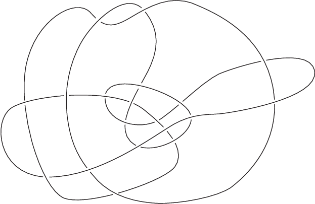
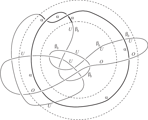
and 34; note that no move $C$ exists in this case.

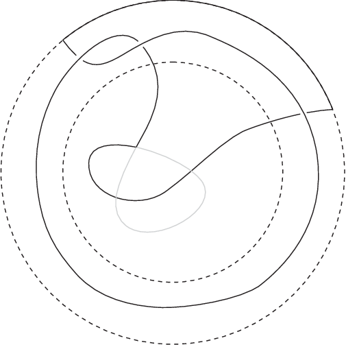
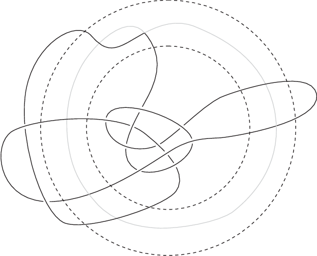
As for the move $C$, the construction implies that $c(D_{0})+c(D_{1})\leqslant c(D)$. Moreover, $c(D_{0})<c(D)$ and $c(D_{1})<c(D)$ except in situations, that one can easily avoid, where one of the $D_{i}$’s is actually $D$.

We conclude by remarking that we do not know whether ${\widetilde{C}}$ is actually essential: all the the knot diagrams we have used so far as tests for our algorithm were completely simplified in a monotonic fashion using the moves $Z_{1,2,3}$ and $C$ only. (For the diagram of Fig. 33 a $C$ appears after some $Z_{1,2,3}$.)

References

- [1] J. Birman, M. D. Hirsch, A new algorithm for recognizing the unknot, Geom. Top. 2 (1998), 175-220.
- [2] J. Birman, W. Menasco, Studying links via closed braids IV: Composite links and split links, Invent. Math. 102 (1990), 115-139.
- [3] J. Birman, W. Menasco, Studying links via closed braids V: Closed braid representatives of the unlink, Trans. Amer. Math. Soc. 329 (1992), 585-606.
- [4] H. Chuichiro, H. Miwa, Unknotting number and number of Reidemeister moves needed for unlinking, Topology Appl. 159 (2012), 1467-1474.
- [5] J.-W. Chung, X.-S. Lin, On the bridge number of knot diagrams with minimal crossings, Math. Proc. Camb. Philos. Soc. 137 (2004), 617-632.
- [6] A. Coward, M. Lackenby, An upper bound on Reidemeister moves, Amer. J. Math. 136 (2014), 1023-1066.
- [7] P. Cromwell, Embedding knots and links in an open book I: Basic properties, Topology Appl. 64 (1995), 37-58.
- [8] I. A. Dynnikov, Three-page link presentation and an untangling algorithm, In: “Proc. of the International Conference Low-Dimensional Topology and Combinatorial Group Theory, Chelyabinsk, July 31-August 7, 1999,” Kiev, 2000, pp. 112-130.
- [9] I. A. Dynnikov, Arc-presentations of links. Monotonic simplification, Fundam. Math. 190 (2006), 29-76.
- [10] A. Enrich, L. Kauffman, Unknotting unknots, Amer. Math. Monthly 121 (2014), 379-390.
- [11] B. Foley, Automated Reidemeister moves: a numerical approach to the unknotting problem, To appear in “Proceedings of Midstates Conference for Undergraduate Research in Computer Science and Mathematics”.
- [12] S. Galatolo, On a problem of effective knot theory, Atti Accad. Naz. Lincei Cl. Sci. Fis. Mat. Natur. Rend. Lincei (9) Mat. Appl. 9 (1998), 299-306.
- [13] H. Gruber, Estimates for the minimal crossing number, arXiv:math/0303273v3.
- [14] J. Hass, J. Lagarias, The number of Reidemeister moves needed for unknotting, J. Amer. Math. Soc. 14 (2001), 399-428 (electronic).
- [15] J. Hass, T. Nowik, Unknot diagrams requiring a quadratic number of Reidemeister moves to untangle, Discrete Computut. Geom. 44 (2010), 91-95.
- [16] A. Henrich, L. H. Kauffman, Unknotting unknots, Amer. Math Monthly 121 (2014), 379-390.
- [17] J. Hoste, The enumeration and classification of knots and links, In: “The Handbook of Knot Theory,” (W. W. Menasco, M. B. Thistlethwaite, eds.), Elsevier, Amsterdam, 2005, pp. 209-232.
- [18] J. Hoste, P. D. Shanahan, Boundary slopes of 2-bridge links determine the crossing number, Kobe J. Math. 24 (2007), 21-39.
- [19] L. H. Kauffman, S. Lambropoulou, Hard unknots and collapsing tangles, In: “Introductory Lectures on Knot Theory” (L. H. Kauffman et al., eds.) Series on Knots and Everything, Vol. 46, World Scientific, Hackensack, NJ, 2012, pp. 187-247.
- [20] A. Kazantsev, Monotonic simplification of arc-presentations of some satellite knots, Russ. Math. Surv. 65 (2010), 785-787.
- [21] S. King, Crossing number of links formed by edges of a triangulation, J. Knot Theory Ramifications 12 (2003), 281-286.
- [22] M. Lackenby, The crossing number of composite knots, J. Topol. 2 (2009), 747-768.
- [23] M. Lackenby, The crossing number of satellite knots, Algebr. Geom. Topol. 14 (2014), 2379-2409.
- [24] M. Lackenby, A polynomial upper bound on Reidemeister moves, arXiv:1302.0180v2, to appear in Ann. of Math.
- [25] Y. Ohyama, On the minimal crossing number and the braid index of links, Canad. J. Math. 45 (1993), 117-131.
- [26] V. V. Prasolov, A. B. Sossinsky, “Knots, Links, Braids and 3-Manifolds. An Introduction to the New Invariants in Low-Dimensional Topology,” Translations of Mathematical Monographs Vol. 154, American Mathematical Society, Providence, RI, 1997.
- [27] D. Rolfsen, “Knots and Links,” Publish or Perish, Berkeley, CA, 1976.
- [28] A. Stoimenow, Tait’s conjectures and odd crossing number of amphicheiral knots, Bull. Amer. Math. Soc. (NS) 45 (2008), 285-291.
- [29] A. Zanellati, www.zanellati.it, personal web page.
adolfo@zanellati.it
Dipartimento di Matematica
Università di Pisa
Largo Bruno Pontecorvo, 5
56127 PISA – Italy
petronio@dm.unipi.it