STFT Phase Retrieval: Uniqueness Guarantees and Recovery Algorithms
Abstract
The problem of recovering a signal from its Fourier magnitude is of paramount importance in various fields of engineering and applied physics. Due to the absence of Fourier phase information, some form of additional information is required in order to be able to uniquely, efficiently and robustly identify the underlying signal. Inspired by practical methods in optical imaging, we consider the problem of signal reconstruction from the Short-Time Fourier Transform (STFT) magnitude. We first develop conditions under which the STFT magnitude is an almost surely unique signal representation. We then consider a semidefinite relaxation-based algorithm (STliFT) and provide recovery guarantees. Numerical simulations complement our theoretical analysis and provide directions for future work.
Index Terms:
Short-Time Fourier Transform (STFT), Phase Retrieval, Super-Resolution, Semidefinite Relaxation.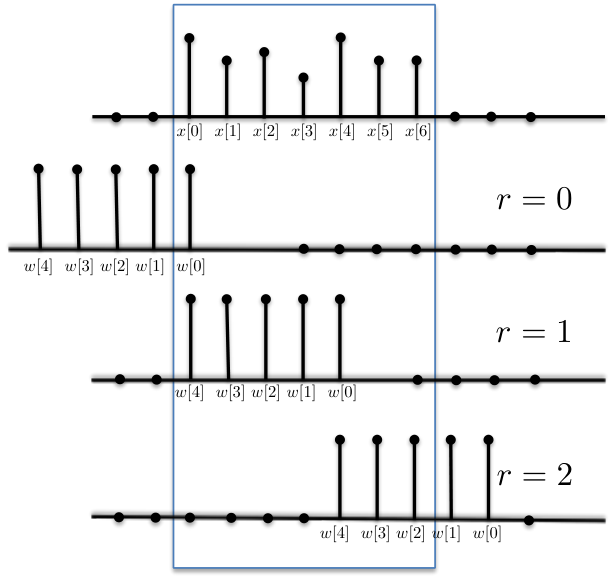
I Introduction
In many physical measurement systems, the measurable quantity is the magnitude-square of the Fourier transform of the underlying signal. The problem of reconstructing a signal from its Fourier magnitude is known as phase retrieval [1, 2]. This reconstruction problem is one with a rich history and occurs in many areas of engineering and applied physics such as optics [3], X-ray crystallography [4], astronomical imaging [5], speech recognition [6], computational biology [7], blind channel estimation [8] and more. We refer the readers to [9, 10, 11] for a comprehensive survey of classical approaches. Recent reviews can be found in [12, 13].
It is well known that phase retrieval is an ill-posed problem [14]. In order to be able to uniquely identify the underlying signal, various methods have been explored, which can be broadly classified into two categories: (i) Additional prior information: common approaches include bounds on the support of the signal [9, 10, 11] and sparsity constraints [17, 19, 24, 20, 18, 23, 21, 22]. (ii) Additional magnitude-only measurements: popular examples include the use of structured illuminations and masks [25, 26, 27, 24, 28, 29, 30], and Short-Time Fourier Transform (STFT) magnitude measurements [31, 34, 35, 33, 32, 37, 39, 36, 38].
We consider STFT phase retrieval, which is the problem of reconstructing a signal from its STFT magnitude. In some applications of phase retrieval, it is easy to obtain such measurements. One example is Frequency Resolved Optical Gating (FROG), which is a general method for measuring ultrashort laser pulses [31]. Fourier ptychography [32, 33, 34], a technology which has enabled X-ray, optical and electron microscopy with increased spatial resolution without the need for advanced lenses, is another popular example. In applications such as speech processing, it is natural to work with the STFT instead of the Fourier transform as the spectral content of speech changes over time [35]. The key idea, when using STFT measurements, is to introduce redundancy in the magnitude-only measurements by maintaining a substantial overlap between adjacent short-time sections. This mitigates the uniqueness and algorithmic issues of phase retrieval.
In this work, our contribution is two-fold:
(i) Uniqueness guarantees: Researchers have previously developed conditions under which the STFT magnitude uniquely identifies signals (up to a global phase). However, either prior information on the signal is assumed in order to provide the guarantees, or the guarantees are limited. For instance, the results provided in [37] require exact knowledge of a small portion of the underlying signal. In [39], the guarantees developed are for the setup in which adjacent short-time sections differ in only one index. These limitations are primarily due to a small number of adversarial signals which cannot be uniquely identified from their STFT magnitude. Here, in contrast, we develop conditions under which the STFT magnitude is an almost surely unique signal representation. In particular, we show that, with the exception of a set of signals of measure zero, non-vanishing signals can be uniquely identified (up to a global phase) from their STFT magnitude if adjacent short-time sections overlap (Theorem III.1). We then extend this result to incorporate sparse signals which have a limited number of consecutive zeros (Corollary III.1).
(ii) Recovery algorithms: Researchers have previously developed efficient iterative algorithms based on classic optimization frameworks to solve the STFT phase retrieval problem. Examples include the Griffin-Lim (GL) algorithm [38] and STFT-GESPAR for sparse signals [39]. While these techniques work well in practice, they do not have theoretical guarantees. In [36] and [43], a semidefinite relaxation-based STFT phase retrieval algorithm, called STliFT (see Algorithm 1 below), was proposed. In this work, we conduct extensive numerical simulations and provide theoretical guarantees for STliFT. In particular, we conjecture that STliFT can recover most non-vanishing signals (up to a global phase) from their STFT magnitude if adjacent short-time sections differ in at most half the indices (Conjecture IV.1). When this condition is satisfied, we argue that one can super-resolve (i.e., discard high frequency measurements) and reduce the number of measurements to , where is the length of the complex signal. Therefore, STliFT recovers most non-vanishing signals uniquely, efficiently and robustly, using an order-wise optimal number of phaseless measurements.
We prove this conjecture for the setup in which the exact knowledge of a small portion of the underlying signal is available (Theorem IV.1). For particular choices of STFT parameters, this portion vanishes asymptotically, due to which this setup is asymptotically reasonable. We also prove this conjecture for the case in which adjacent short-time sections differ in only one index (Theorem IV.2). We then extend these results to incorporate sparse signals which have a limited number of consecutive zeros (Corollary IV.1).
The rest of the paper is organized as follows. In Section 2, we mathematically formulate STFT phase retrieval and establish our notation. We present uniqueness guarantees in Section 3. Section 4 considers the STliFT algorithm and provides recovery guarantees. Numerical simulations are presented in Section 5. Section 6 concludes the paper.
II Problem Setup
Let be a signal of length and be a window of length . The STFT of with respect to , denoted by , is defined as:
| (1) |
for and , where the parameter denotes the separation in time between adjacent short-time sections and the parameter denotes the number of short-time sections considered.
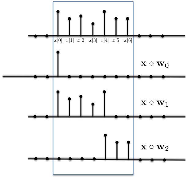
The STFT can be interpreted as follows: Suppose denotes the signal obtained by shifting the flipped window by time units (i.e., ) and is the Hadamard (element-wise) product operator. The th column of , for , corresponds to the point DFT of . In essence, the window is flipped and slid across the signal (see Figure 1 for a pictorial representation), and corresponds to the Fourier transform of the windowed signal recorded at regular intervals. This interpretation is known as the sliding window interpretation.
Let be the measurements corresponding to the magnitude-square of the STFT of with respect to so that . Let , for , be the diagonal matrix with diagonal elements . STFT phase retrieval can be mathematically stated as:
| (2) | ||||
for and , where is the conjugate of the th column of the point DFT matrix and is the inner product operator. In fact, STFT phase retrieval can be equivalently stated by only considering the measurements corresponding to and , for any parameter satisfying (see Section VII for details). This equivalence significantly reduces the number of measurements when , which is typically the case in practical methods. In Section 4, we further reduce the number of measurements per short-time section through super-resolution. In particular, we consider the setup with and .
We use the following definitions: A signal is said to be non-vanishing if for all . Similarly, a window is said to be non-vanishing if for all . Further, a signal is said to be sparse if it is not non-vanishing, i.e., for at least one .
| Uniqueness if the first samples are known a priori, and is non-vanishing [37] | |
|---|---|
| Non-vanishing signals { for all } | Uniqueness up to a global phase if , , coprime with and mild conditions on [39] |
| Uniqueness up to a global phase for almost all signals if and is non-vanishing [This work] | |
| Uniqueness for signals with at most consecutive zeros if the first samples, starting from the first non-zero sample, are known a priori, and is non-vanishing [37] | |
| Sparse signals { for at least one } | No uniqueness for most signals with consecutive zeros [39] |
| Uniqueness up to a global phase and time-shift for almost all signals with less than consecutive zeros if and is non-vanishing [This work] |
III Uniqueness Guarantees
In this section, we review existing results regarding the uniqueness of STFT phase retrieval and present our uniqueness guarantees. The results are summarized in Table I.
In STFT phase retrieval, the global phase of the signal cannot be determined due to the fact that signals and , for any , always have the same STFT magnitude regardless of the choice of . In contrast, in classic phase retrieval, signals which differ from each other by a global phase, time-shift and/ or conjugate-flip (together called trivial ambiguities) cannot be distinguished from each other as they have the same Fourier magnitude [17, 21, 12].
Observe that is a necessary condition in order to be able to uniquely identify most signals. If , then the STFT magnitude does not contain any information from some locations of the signal. When , adjacent short-time sections do not overlap and hence STFT phase retrieval is equivalent to a series of non-overlapping instances of classic phase retrieval. Since there is no way of determining the relative phase, time-shift or conjugate-flip between the windowed signals corresponding to the various short-time sections, most signals cannot be uniquely identified. For example, suppose is chosen such that and for all . Consider the signal of length . Signals and have the same STFT magnitude. In fact, more generally, signals and , for any , have the same STFT magnitude.
III-A Non-vanishing signals
For some specific choices of , it has been shown that all non-vanishing signals can be uniquely identified from their STFT magnitude up to a global phase. In [39], it is proven that the STFT magnitude uniquely identifies non-vanishing signals up to a global phase for if the window is chosen such that the point DFT of is non-vanishing, and is coprime with . In [37], the authors prove that if the first samples are known a priori, then the STFT magnitude can uniquely identify non-vanishing signals for any if the window is chosen such that it is non-vanishing and .
In this work, we prove the following result for non-vanishing signals:
Theorem III.1.
Almost all non-vanishing signals can be uniquely identified (up to a global phase) from their STFT magnitude if satisfy
- (i)
is non-vanishing
- (ii)
- (iii)
.
Proof.
The proof is based on a technique commonly known as dimension counting. The outline is as follows (see Section VIII for details):
Consider the short-time sections and . Since adjacent short-time sections overlap (due to ), there exists at least one index, say , where both and have non-zero values.
Since , there can be at most distinct windowed signals (up to a phase) that have the same Fourier magnitude [14]. Consequently, is restricted to values by the th column of the STFT magnitude (let denote the set of these values). Similarly, is restricted to values by the th column of the STFT magnitude (denote the set of these values by ).
By construction, as the STFT magnitude is generated by an underlying signal , i.e., . Using Lemma VIII.1 and Theorem VIII.1, we show that, for almost all non-vanishing signals, has cardinality one. In other words, is uniquely identified (up to a phase) almost surely.
Since adjacent short-time sections overlap, non-vanishing signals are uniquely identified up to a global phase from the knowledge of (up to a phase) for if is non-vanishing. ∎
III-B Sparse signals
While the aforementioned results provide guarantees for non-vanishing signals, they do not say anything about sparse signals. Reconstruction of sparse signals involves certain challenges which are not encountered in the reconstruction of non-vanishing signals.
The following example is provided in [39] to show that the time-shift ambiguity cannot be resolved for some classes of sparse signals and some choices of : Suppose is chosen such that , is a multiple of and for all . Consider a signal of length such that it has non-zero values only within an interval of the form for some integers and . The signal obtained by time-shifting by units (i.e., ) has the same STFT magnitude. The issue with this class of sparse signals is that the STFT magnitude is identical to the Fourier magnitude because of which the time-shift and conjugate-flip ambiguities cannot be resolved.
It is also shown that some sparse signals cannot be uniquely recovered even up to the trivial ambiguities for some choices of using the following example: Consider two non-overlapping intervals such that , and take a signal supported on and supported on . The magnitude-square of the STFT of and of are equal for any choice of . The difficulty with this class of sparse signals is that the two intervals with non-zero values are separated by a distance greater than because of which there is no way of establishing relative phase using a window of length .
These examples demonstrate the fact that sparse signals are harder to recover than non-vanishing signals in this setup. Since the aforementioned issues are primarily due to a large number of consecutive zeros, the uniqueness guarantees for non-vanishing signals have been extended to incorporate sparse signals with limits on the number of consecutive zeros. In [37], it was shown that if consecutive samples, starting from the first non-zero sample, are known a priori, then the STFT magnitude can uniquely identify signals with less than consecutive zeros for any if the window is chosen such that it is non-vanishing and .
Below, we extend Theorem III.1 to prove the following result for sparse signals:
Corollary III.1.
Almost all sparse signals with less than consecutive zeros can be uniquely identified (up to a global phase and time-shift) from their STFT magnitude if satisfy
- (i)
is non-vanishing
- (ii)
- (iii)
.
Proof.
The bound on consecutive zeros ensures the following: For sufficient pairs of adjacent short-time sections, there is at least one index among the overlapping and non-overlapping indices respectively, where the underlying signal has a non-zero value. We refer the readers to Section IX for details. ∎
IV Recovery Algorithms
The classic alternating projection algorithm to solve phase retrieval [9] has been adapted to solve STFT phase retrieval by Griffin and Lim [38]. To this end, STFT phase retrieval is reformulated as the following least-squares problem:
| (3) |
The Griffin-Lim (GL) algorithm attempts to minimize this objective by starting with a random initialization and imposing the time domain and STFT magnitude constraints alternately using projections. The objective is shown to be monotonically decreasing as the iterations progress. An important feature of the GL algorithm is its empirical ability to converge to the global minimum when there is substantial overlap between adjacent short-time sections. However, no theoretical recovery guarantees are available. To establish such guarantees, we rely on a semidefinite relaxation approach.
IV-A Semidefinite relaxation-based algorithm
Semidefinite relaxation has enjoyed considerable success in provably and stably solving several quadratic-constrained problems [40, 41, 42]. The steps to formulate such problems as a semidefinite program (SDP) are as follows: (i) Embed the problem in a higher dimensional space using the transformation , a process which converts the problem of recovering a signal with quadratic constraints into a problem of recovering a rank-one matrix with affine constraints. (ii) Relax the rank-one constraint to obtain a convex program.
If the convex program has a unique solution , then is the unique solution to the quadratic-constrained problem (up to a global phase). Many recent results in related problems like generalized phase retrieval [42] and phase retrieval using random masks [28, 29] suggest that one can provide conditions, which when satisfied, ensure that the convex program has a unique solution .
A semidefinite relaxation-based STFT phase retrieval algorithm, called STliFT, was explored in [36] and [43]. The details of the algorithm are provided in Algorithm 1. In the following, we develop conditions on which ensure that the convex program (4) has as the unique solution. Consequently, under these conditions, STliFT uniquely recovers the underlying signal up to a global phase.
Input: STFT magnitude measurements for and , .
Output: Estimate of the underlying signal .
- •
Obtain by solving:
(4) for and .
- •
Return , where is the best rank-one approximation of .
Based on extensive numerical simulations, we conjecture the following:
Conjecture IV.1.
The convex program (4) has a unique solution , for most non-vanishing signals , if
- (i)
is non-vanishing
- (ii)
- (iii)
.
The number of phaseless measurements considered can be calculated as follows: The total number of short-time sections is . For each short-time section, phaseless measurements are sufficient. Hence, the total number of phaseless measurements is . Consequently, when , this number is , which is order-wise optimal. In fact, in generalized phase retrieval, it is conjectured that phaseless measurements are necessary [45].
The proof techniques used in [28] and [42] are not applicable in the STFT setup. In [28] and [42], the measurement vectors are chosen from a random distribution such that they satisfy the restricted isometry property. Furthermore, the randomness in the measurement vectors is used to construct approximate dual certificates based on concentration inequalities. In the STFT setup, testing whether the given measurement vectors satisfy the restricted isometry property is difficult. Also, due to the lack of randomness in the measurement vectors, a different approach is required to construct dual certificates.
In the following, we develop a proof technique for the STFT setup, and use it to prove Conjecture IV.1, with additional assumptions.


Theorem IV.1.
The convex program (4) has a unique feasible matrix , for almost all non-vanishing signals , if
- (i)
is non-vanishing
- (ii)
- (iii)
- (iv)
for is known a priori.
Proof.
See Section X. ∎
While it is sufficient to show that (4) has a unique solution , observe that Theorem IV.1 ensures that (4) has a unique feasible matrix. This is a stronger condition, and as a consequence, the choice of the objective function does not matter in the noiseless setting. While this might suggest that the requirements of the setup are strong, we argue that it is not the case. In fact, this phenomenon is also observed in generalized phase retrieval (Section in [42]) and phase retrieval using random masks (Theorem in [28]).
Theorem IV.1 assumes prior knowledge of the first samples, i.e., half of the second short-time section is required to be known a priori. This is not a lot of prior information if , which is typically the case. When , the fraction of the signal that is required to be known a priori is less than , which tends to as .
Theorem IV.2.
The convex program (4) has a unique feasible matrix , for almost all non-vanishing signals , if
- (i)
is non-vanishing
- (ii)
- (iii)
- (iv)
.
Proof.
This is a direct consequence of Theorem IV.1. The value of (and hence , without loss of generality) can be inferred from the STFT magnitude if . ∎
When , the number of phaseless measurements is , which is again order-wise optimal. For example, when , at most phaseless measurements are considered. Unlike Theorem IV.1, no prior information is necessary.
Corollary IV.1.
The convex program (4) has a unique feasible matrix , for almost all sparse signals which have at most consecutive zeros, if
- (i)
is non-vanishing
- (ii)
- (iii)
- (iv)
Either or for is known a priori, where is the smallest index such that .
Proof.
See Section X. ∎
IV-B Noisy Setting
In practice, the measurements are contaminated by additive noise, i.e., the measurements are of the form
for and , where is the additive noise corresponding to the th short-time section and . STliFT, in the noisy setting, can be implemented as follows: Suppose for all . The constraints in the convex program (4) can be replaced by
| (5) |
for . We recommend the use of trace minimization as the objective function. Numerical simulations strongly suggest that STliFT can recover most non-vanishing signals stably in the noisy setting under certain conditions. The details of the simulations are provided in the following section.
V Numerical Simulations
In this section, we demonstrate the empirical abilities of STliFT using numerical simulations.
In the first set of simulations, we evaluate the performance of STliFT as a function of window and shift lengths. We choose , and vary . For each choice of , we consider phaseless measurements and perform trials. In every trial, we choose a random signal such that the values in each location are drawn from an i.i.d. standard complex normal distribution. We select the window such that for all . The probability of successful recovery as a function of is plotted in Fig. 2a.
Observe that STliFT successfully recovers the underlying signal with very high probability when and fails with very high probability when . The choice of uses only six short-time sections and STliFT recovers the underlying signal with very high probability, which, given the limited success of semidefinite relaxation-based algorithms in the Fourier phase retrieval setup, is very encouraging.
In the second set of simulations, we evaluate the performance of STliFT as a function of shift length and measurements per short-time section. We choose and , and vary . For each choice of , we perform trials as before. The probability of successful recovery as a function of is plotted in Fig. 2b. Observe that recovery is successful even in the regime.
In the third set of simulations, we evaluate the performance of STliFT in the noisy setting. We choose , the rest of the parameters are the same as the first set of simulations. The normalized mean-squared error, given by
| (6) |
is plotted as a function of SNR in Fig. 3. The linear relationship between them shows that STliFT stably recovers the underlying signal in the presence of noise. Also, it can be observed that the choices of which correspond to significant overlap between adjacent short-time sections tend to recover signals more stably compared to values of which correspond to less overlap, which is not surprising.
VI Conclusions and Future Directions
In this work, we considered the STFT phase retrieval problem. We showed that, if , then almost all non-vanishing signals can be uniquely identified from their STFT magnitude (up to a global phase), and extended this result to incorporate sparse signals which have less than consecutive zeros.
For , we conjectured that most non-vanishing signals can be recovered (up to a global phase) by a semidefinite relaxation-based algorithm (STliFT). When , through super-resolution, we reduced the number of phaseless measurements to . We proved this conjecture for the setup in which the first samples are known, and for the case in which . We argued that the additional assumptions are asymptotically reasonable when , which is typically the case in practical methods. We then extended these results to incorporate sparse signals which have at most consecutive zeros.
Natural directions for future study include a proof of this conjecture without the additional assumptions, and a stability analysis in the noisy setting. Also, a thorough analysis of the phase transition at will provide a more complete characterization of STliFT.
Acknowledgements: We would like to thank Mordechai Segev and Oren Cohen for introducing us to the STFT phase retrieval problem, and for many insightful discussions.
References
- [1] A. L. Patterson, “A Fourier series method for the determination of the components of interatomic distances in crystals,” Physical Review 46, no. 5 (1934): 372.
- [2] A. L. Patterson, “Ambiguities in the X-ray analysis of crystal structures,” Physical Review 65, no. 5-6 (1944): 195.
- [3] A. Walther, “The question of phase retrieval in optics,” Journal of Modern Optics 10, no. 1 (1963): 41-49.
- [4] R. P. Millane, “Phase retrieval in crystallography and optics,” JOSA A 7, no. 3 (1990): 394-411.
- [5] J. C. Dainty and J. R. Fienup, “Phase retrieval and image reconstruction for astronomy,” Image Recovery: Theory and Application (1987): 231-275.
- [6] L. Rabiner and B. H. Juang, “Fundamentals of speech recognition,” Prentice Hall (1993).
- [7] M. Stefik, “Inferring DNA structures from segmentation data,” Artificial Intelligence 11, no. 1 (1978): 85-114.
- [8] B. Baykal, “Blind channel estimation via combining autocorrelation and blind phase estimation,” IEEE Transactions on Circuits and Systems 51, no. 6 (2004): 1125-1131.
- [9] R. W. Gerchberg and W. O. Saxton, “A practical algorithm for the determination of the phase from image and diffraction plane pictures,” Optik 35 (1972): 237.
- [10] J. R. Fienup, “Phase retrieval algorithms: A comparison,” Applied Optics 21, no. 15 (1982): 2758-2769.
- [11] H. H. Bauschke, P. L. Combettes and D. R. Luke, “Phase retrieval, error reduction algorithm, and Fienup variants: A view from convex optimization,” JOSA A 19, no. 7 (2002): 1334-1345.
- [12] Y. Shechtman, Y. C. Eldar, O. Cohen, H. N. Chapman, J. Miao and M. Segev, “Phase retrieval with application to optical imaging,” IEEE Signal Processing Magazine 32, no. 3 (2015): 87-109.
- [13] K. Jaganathan, Y. C. Eldar and B. Hassibi, “Phase retrieval: An overview of recent developments,” arXiv:1510.07713 (2015).
- [14] E. M. Hofstetter, “Construction of time-limited functions with specified autocorrelation functions,” IEEE Transactions on Information Theory 10, no. 2 (1964): 119-126.
- [15] M. H. Hayes and J. H. McClellan, “Reducible polynomials in more than one variable,” Proceedings of the IEEE 70, no. 2 (1982): 197-198.
- [16] J. M. Ortega and W. C. Rheinboldt, “Iterative solution of nonlinear equations in several variables,” Vol. 30. Siam (1970).
- [17] Y. M. Lu and M. Vetterli, “Sparse spectral factorization: Unicity and reconstruction algorithms,” IEEE International Conference on Acoustics, Speech and Signal Processing (2011): 5976-5979.
- [18] A. Szameit, Y. Shechtman, E. Osherovich, E. Bullkich, P. Sidorenko, H. Dana, S. Steiner, E. B. Kley, S. Gazit, T. Cohen-Hyams, S. Shoham, M. Zibulevsky, I. Yavneh, Y. C. Eldar, O. Cohen and M. Segev, “Sparsity-based single-shot subwavelength coherent diffractive imaging,” Nature Materials [Online], Supplementary Info (2012).
- [19] S. Mukherjee and C. Seelamantula, “An iterative algorithm for phase retrieval with sparsity constraints: Application to frequency domain optical coherence tomography,” IEEE International Conference on Acoustics, Speech and Signal Processing (2012): 553Ð556.
- [20] Y. Shechtman, Y. C. Eldar, A. Szameit and M. Segev, “Sparsity based sub-wavelength imaging with partially incoherent light via quadratic compressed sensing,” Optics Express 19 (2011): 14807-14822.
- [21] K. Jaganathan, S. Oymak and B. Hassibi, “Recovery of sparse 1-D signals from the magnitudes of their Fourier transform,” IEEE International Symposium on Information Theory Proceedings (2012): 1473-1477.
- [22] K. Jaganathan, S. Oymak and B. Hassibi, “Sparse phase retrieval: Uniqueness guarantees and recovery algorithms,” arXiv:1311.2745 (2015).
- [23] Y. Shechtman, A. Beck and Y. C. Eldar, “GESPAR: Efficient phase retrieval of sparse signals,” IEEE Transactions on Signal Processing 62, no. 4 (2014): 928-938.
- [24] E. J. Candes, Y. C. Eldar, T. Strohmer and V. Voroninski, “Phase retrieval via matrix completion,” SIAM Journal on Imaging Sciences 6.1 (2013): 199-225.
- [25] Y. J. Liu et al. “Phase retrieval in X-ray imaging based on using structured illumination,” Physical Review A 78, no. 2 (2008): 023817.
- [26] I. Johnson, K. Jefimovs, O. Bunk, C. David, M. Dierolf, J. Gray, D. Renker and F. Pfeiffer, “Coherent diffractive imaging using phase front modifications,” Physical review letters 100, no. 15 (2008): 155503.
- [27] E. G. Loewen and E. Popov, “Diffraction gratings and applications,” CRC Press (1997).
- [28] E. J. Candes, X. Li, and M. Soltanolkotabi, “Phase retrieval from coded diffraction patterns,” Applied and Computational Harmonic Analysis (2014).
- [29] D. Gross, F. Krahmer, and R. Kueng, “Improved recovery guarantees for phase retrieval from coded diffraction patterns”, arXiv:1402.6286 (2014).
- [30] K. Jaganathan, Y. C. Eldar and B. Hassibi, “Phase retrieval with masks using convex optimization,” IEEE International Symposium on Information Theory Proceedings (2015): 1655-1659 .
- [31] R. Trebino, “Frequency-resolved optical gating: The measurement of ultrashort laser pulses,” Springer (2002).
- [32] M. J. Humphry, B. Kraus, A. C. Hurst, A. M. Maiden, J. M. Rodenburg, “Ptychographic electron microscopy using high-angle dark-field scattering for sub-nanometre resolution imaging,” Nature Communications 3 (2012).
- [33] J. M. Rodenburg, “Ptychography and related diffractive imaging methods,” Advances in Imaging and Electron Physics 150 (2008): 87-184.
- [34] G. Zheng, R. Horstmeyer and C. Yang, “Wide-field, high-resolution Fourier ptychographic microscopy,” Nature photonics 7, no. 9 (2013): 739-745.
- [35] J. S. Lim and A. V. Oppenheim, “Enhancement and bandwidth compression of noisy speech,” Proceedings of the IEEE 67.12 (1979): 1586-1604.
- [36] K. Jaganathan, Y. C. Eldar and B. Hassibi, “Recovering signals from the short-time Fourier transform magnitude,” IEEE International Conference on Acoustics, Speech and Signal Processing (2015).
- [37] S. H. Nawab, T. F. Quatieri, and J. S. Lim, “Signal reconstruction from short-time Fourier transform magnitude,” IEEE Transactions on Acoustics, Speech and Signal Processing 31, no. 4 (1983): 986-998.
- [38] D. Griffin and J. S. Lim, “Signal estimation from modified short-time Fourier transform,” IEEE Transactions on Acoustics, Speech and Signal Processing 32, no. 2 (1984): 236-243.
- [39] Y. C. Eldar, P. Sidorenko, D. G. Mixon, S. Barel and O. Cohen, “Sparse phase retrieval from short-time Fourier measurements,” IEEE Signal Processing Letters 22, no. 5 (2015): 638-642.
- [40] M. X. Goemans and D. P. Williamson, “Improved approximation algorithms for maximum cut and satisfiability problems using semidefinite programming,” Journal of the ACM (JACM), 42(6), 1115-1145 (1995).
- [41] I. Waldspurger, A. d’Aspremont and S. Mallat, “Phase recovery, maxcut and complex semidefinite programming,” Mathematical Programming 149.1-2 (2015): 47-81.
- [42] E. J. Candes, T. Strohmer, and V. Voroninski, “Phaselift: Exact and stable signal recovery from magnitude measurements via convex programming,” Communications on Pure and Applied Mathematics 66, no. 8 (2013): 1241-1274.
- [43] D. L. Sun and J. O. Smith, “Estimating a signal from a magnitude spectrogram via convex optimization,” arXiv:1209.2076 (2012).
- [44] L. R. Rabiner and R. W. Schafer, “Digital processing of speech signals,” Prentice Hall, (1978).
- [45] R. Balan, P. Casazza and D. Edidin, “On signal reconstruction without phase,” Applied and Computational Harmonic Analysis 20, no. 3 (2006): 345-356.
- [46] E. J. Candes and T. Tao, “Decoding by linear programming,” Information Theory, IEEE Transactions on 51, no. 12 (2005): 4203-4215.
- [47] E. J. Candes and B. Recht, “Exact matrix completion via convex optimization,” Foundations of Computational mathematics 9.6 (2009): 717-772.
- [48] B. Recht, M. Fazel and P. Parrilo, “Guaranteed minimum-rank solutions of linear matrix equations via nuclear norm minimization,” SIAM Review 52, no. 3 (2010): 471-501.
- [49] K. Jaganathan, S. Oymak and B. Hassibi, “Sparse phase retrieval: Convex algorithms and limitations,” Information Theory Proceedings (ISIT), IEEE International Symposium on (2013): 1022-1026.
- [50] R. A. Horn and C. R. Johnson, “Matrix analysis,” Cambridge university press (2012).
- [51] L. Vandenberghe and S. Boyd, “Semidefinite programming,” SIAM review (1996): 49-95.
Appendix
VII Equivalent definition of stft phase retrieval
Since we consider point DFT and satisfies , STFT phase retrieval can be equivalently stated in terms of the short-time autocorrelation [14]:
| (7) | ||||
| subject to | ||||
for and .
The knowledge of the short-time autocorrelation is sufficient for all the guarantees provided in this paper. Note that the th column of and the th column of are Fourier pairs. Hence, for a particular , if for is available, then for can be calculated by taking an inverse Fourier transform. The following lemma shows that phaseless measurements per short-time section are sufficient to infer the short-time autocorrelation.
Lemma VII.1.
for is sufficient to calculate for .
Proof.
If the window length is , then has non-zero values only in the interval and . Let be the signal obtained by circularly shifting by rows, so that has non-zero values only in the interval . Since the submatrix of the point DFT matrix obtained by considering the first columns and any rows is invertible (the Vandermonde structure is retained), for and for are related by an invertible matrix. Note that for can be trivially calculated from for . ∎
Consequently, if the point DFT is used and is satisfied, the affine constraints in (4) can be rewritten in terms of and as:
VIII Proof of Theorem III.1
The symbol is used to denote equality up to a global phase and time-shift44 4 For non-vanishing signals, there is no ambiguity due to time-shift.. We say that two signals and are distinct if , and equivalent if .
Let denote the set of all distinct non-vanishing complex signals of length . is a manifold of dimension , i.e., locally resembles a real dimensional space. This can be seen as follows: In order to discard the global phase of non-vanishing signals, we can assume that is real and positive at one index , without loss of generality. Hence, can take any value in , and , for each not equal to , can take any value in , due to the one-to-one correspondence between and .
Let be the set of distinct non-vanishing complex signals which cannot be uniquely identified from their STFT magnitude if is chosen such that it is non-vanishing and . We show that has measure zero in . In order to do so, our strategy is as follows:
We first characterize using Lemma VIII.1. In particular, we show that is a finite union of images of continuously differentiable maps from to . Since is a manifold of dimension , the following result completes the proof:
Theorem VIII.1 ([16], Chapter 5).
If is a continuously differentiable map, then the image of has measure zero in , provided .
We use the following notation in this section: If is a signal of length , then such that and outside the interval . The vector denotes the conjugate-flipped version of , i.e., . Let and denote the smallest and largest index where the windowed signal has a non-zero value respectively.
Lemma VIII.1.
Consider two signals of length which have the same STFT magnitude. If the window is chosen such that it is non-vanishing and , then, for each , there exists signals and , of lengths and respectively, such that
- (i)
- (ii)
- (iii)
and
where is the convolution operator. Further, there exists at least one such that
- (iv)
, is real and positive.
Proof.
In Lemma of [22], it is shown that if two non-equivalent signals of length have the same Fourier magnitude and if the DFT dimension is at least (this would imply that they have the same autocorrelation), then there exists signals and , of lengths and respectively, such that one signal can be decomposed as and the other signal can be decomposed as . For each , the th column of the STFT magnitude is equivalent to the Fourier magnitude of the windowed signal . The DFT dimension is , and the windowed signal length is (which is less than or equal to ). Since, for every , and have the same Fourier magnitude, the aforementioned result proves (i).
The conditions (ii) and (iii) are properties of convolution (see Lemma of [22] for details), and therefore hold for every .
Furthermore, if for all , then . Hence, for at least one . For this , since and have the same STFT magnitude, can be assumed to be real and positive without loss of generality. Hence, (iv) holds for at least one . ∎
Consequently, for each , condition (iv) of Lemma VIII.1 holds for at least one . Let denote the set of signals for which and 22 2 When , we consider the short-time section instead of . We show the detailed calculations for the case when short-time section is considered, the arguments are symmetric for .. It suffices to show that for each , and , there exists a set , which is the image of a continuously differentiable map from to .
We first show the arguments for the case as the expressions are simple and provide intuition for the technique. Then, we show the arguments for the case.
The set is constructed as follows: Consider the variables satisfying and , and for . The map from these variables to is the following:
| (8) |
Observe that, for , has two definitions. The variables can admit only those values for which the two definitions have the same value. In the following, we show that there is a one-to-one correspondence between the set of admissible values of the variables and a subset of .
Each , for , can be chosen from . The set of is a subset of , which can be seen as follows: is fixed (see Lemma VIII.1), there are other terms and each can be chosen from .
For each choice of , consider the set of excluding the terms and : is fixed, there are other terms and each can be chosen from . Hence, this set is a subset of .
Since the short-time sections and overlap in the index , and must be consistent in this index, i.e., must satisfy:
| (9) |
Due to Lemma VIII.1, and must also be consistent in this index up to a phase, i.e., must also satisfy:
| (10) |
Observe that is used in (10), due to the fact that the equality is only up to a phase. However, is real and positive (see Lemma VIII.1), due to which (10) fixes .
Consequently, the set of admissible values of the variables, excluding and , is a subset of , as . For each point in this set, and are uniquely determined. It is straightforward to check that the map from this set to is continuously differentiable. Consequently, is the image of a continuously differentiable map from to .
Consider the setup for which . The set of , as earlier, is a subset of .
The short-time sections and overlap in the interval . Let (the number of indices in the overlapping interval). Due to , we have . Hence, for each choice of , must satisfy:
| (11) | ||||
for . In addition, must also satisfy:
| (12) |
If , then the bilinear equations (11) can be written as , where has upper triangular structure with unit diagonal entries, due to which . The set of is a subset of . For each choice of , the terms are fixed by . The constraint (12) fixes the value of , as earlier. Each of the remaining terms of may be chosen from .
Hence, the set of admissible values of the variables, excluding and , is a subset of , due to the fact that (as ). For each point in this set, and are uniquely determined. The rest of the arguments are identical to those of .
If instead, then the bilinear equations (11) can be equivalently written as , the same arguments may be applied to draw the same conclusion. For the setup with , the same arguments hold for the short-time sections and , where is the largest integer such that the short-time sections and overlap (this ensures ).
IX Proof of Corollary III.1
We now extend Theorem III.1 to incorporate sparse signals. Let denote the set of all distinct complex signals of length with a support . Here, is a binary vector of length , such that whenever and whenever . Further, has less than consecutive zeros.
Let denote the set of signals which cannot be uniquely identified from their STFT magnitude if is chosen such that it is non-vanishing and . We show that has measure zero in .
In the proof of Theorem III.1, in order to show dimension reduction, we used the fact that for sufficient pairs of adjacent short-time sections and , the following holds:
(i) There is at least one index in the non-overlapping indices or where the signals and have a non-zero value. This ensures that is not constrained by in general. This condition can be ensured by imposing the constraint that the sparse signal cannot have consecutive zeros.
(ii) There is at least one index in the overlapping indices where the signals and have a non-zero value. This ensures that is constrained by (10) for signals which cannot be uniquely identified by their STFT magnitude. This condition can be ensured by imposing the constraint that the sparse signal cannot have consecutive zeros.
The only difference in the proof is the following: Unlike in the case of non-vanishing signals, there is time-shift ambiguity. Hence, the constraint (12) is replaced by:
| (13) |
for some . This fixes the value of to one of at most values, due to which there is a dimension reduction.
X Proof of Theorem IV.1
We first show the arguments for the case (short-time autocorrelation known) as the expressions are simple and provide intuition. Then, we show the arguments for the case (super-resolution).
The proof strategy is as follows: We begin by focusing our attention on short-time section . We show that the prior information available, along with the affine autocorrelation measurements corresponding to and the positive semidefinite constraint, will ensure that every feasible matrix of (4) satisfies for . We then apply this argument incrementally, i.e., we show that the affine measurements corresponding to short-time section , along with the entries of uniquely determined and the positive semidefinite constraint, will ensure that for , where and denote the smallest and largest index where has a non-zero value respectively. Consequently, the entries along the diagonal and the first off-diagonals of every feasible matrix of (4) match the entries along the diagonal and the first off-diagonals of the matrix . Since the entries are sampled from a rank one matrix with non-zero diagonal entries (i.e., ), there is exactly one positive semidefinite completion, which is the rank one completion [50].
Let be a length subsignal of , and be the submatrix of corresponding to the first rows and columns. We now show that is the only feasible matrix under the constraints of (4).
Since for is known a priori, we have for . Let denote these constraints due to prior information, along with the affine constraints corresponding to . In particular, denotes the following set of constraints:
For each feasible matrix , these set of measurements fix (i) the submatrix, corresponding to the first rows and columns, of (ii) the appropriately weighted sum along the diagonal and each off-diagonal of ( is implicitly used here).
Lemma X.1.
If satisfies , then it is the only positive semidefinite matrix which satisfies .
Proof.
Let be the set of Hermitian matrices of the form
and be its orthogonal complement. The set may be interpreted as the tangent space at to the manifold of Hermitian matrices of rank one. Influenced by [42], we use and to denote the projection of a matrix onto the subspaces and respectively.
Standard duality arguments in semidefinite programming show that the following are sufficient conditions for to be the unique optimizer of (4):
- (i)
Condition 1: .
- (ii)
Condition 2: There exists a dual certificate in the range space of obeying:
- •
- •
- •
.
- •
The proof of this result is based on KKT conditions, and can be found in any standard reference on semidefinite programming (for example, see [51]).
We first show that Condition 1 is satisfied. The set of constraints in due to prior information fix the entries of the first rows and columns of to . Since for some (due to ), we infer that for , for some real constant . Indeed, the equations of the form imply , for some real constant . The equations imply .
The set of constraints in due to the measurements corresponding to , along with for , imply for . Hence, for , implies , which in turn implies .
We next establish Condition 2. For simplicity of notation, we consider the case where for . For a general non-vanishing , the same arguments hold (the Toeplitz matrix considered is appropriately redefined with weights).
The range space of is the set of all matrices which are a sum of the following two matrices: The first matrix can have any value in the submatrix corresponding to the first rows and columns, and has a value zero outside this submatrix (dual of the set of constraints due to prior information). The second matrix has a Toeplitz structure (dual of the measurements corresponding to ).
Suppose is the vector containing the first entries of and is the vector containing the remaining entries of . Here, corresponds to the locations where we have knowledge of the entries and corresponds to the locations where the entries are not determined. Let be a lower triangular Toeplitz matrix satisfying . Such an always exists if is non-zero and the length of is greater than or equal to the length of . Let be any positive semidefinite matrix with rank satisfying . Again, such a always exists (any positive semidefinite matrix with eigenvectors perpendicular to ). Consider the following dual certificate:
| (14) |
Clearly, is in the range space of . Also, by construction. From the Schur complement, it is straightforward to see that and . ∎
We have shown that is the only positive semidefinite matrix which satisfies the prior information and the measurements corresponding to . Redefine and such that is the length subsignal of and is the submatrix of corresponding to the first rows and columns.
We already have for from above. Let denote these constraints, along with the affine constraints corresponding to . Due to , Lemma X.1 proves that is the only psd matrix which satisfies the prior information and the measurements corresponding to . Applying this argument incrementally, the entries along the diagonal and the first off-diagonals of every feasible matrix of (4) match the entries along the diagonal and the first off-diagonals of the matrix .
Sparse signals: The arguments can be seamlessly extended to incorporate sparse signals.
(i) The fact that there exists a unique positive semidefinite completion once the diagonal and the first off-diagonal entries are sampled from holds when has less than consecutive zeros.
(ii) Note that the length of is at most , as it corresponds to the locations in the window where the entries are not determined. Since we know for a priori, where is the smallest index such that , the length of is . Redefine so that it corresponds to the locations in the window where the entries are determined, starting from the smallest index which has a non-zero value in order to ensure . If has at most consecutive zeros, then the length of is at least . Hence, a lower triangular Toeplitz matrix , satisfying , always exists.
:
The range space of the dual certificate is the set of all matrices which are a sum of the following two matrices: The first matrix can have any value in the submatrix corresponding to the first rows and columns, and has a value zero outside this submatrix (dual of the set of constraints due to prior information). The second matrix has the form , where is real-valued for each (dual of the measurements corresponding to ).
Let be a vector that satisfies:
- (i)
,
- (ii)
for
- (iii)
.
These constraints together can be written as . When , the matrix is square or wide, and almost always (pseudo) invertible. This can be seen as follows: the determinant of is a polynomial function of the entries of , due to which it is either always zero or almost surely non-zero. By substituting and for , it is straightforward to check that the determinant is non-zero. Hence, such an almost always exists.
If the last row in (14) is chosen as , then we have: (i) The lower right block is an identity matrix. (ii) is satisfied. (iii) Since is a real vector, satisfies . Therefore, is in the range space of where is real-valued, due to which the resulting second matrix is in the range space of .
Therefore, satisfies all the requirements. The arguments are applied incrementally as earlier, with for .
![[Uncaptioned image]](1508.02820v3/kishore_photo.jpg) |
Kishore Jaganathan was born in Tamil Nadu, India, in 1989. He received the B.Tech degree from Indian Institute of Technology, Madras in 2010, and the M.S. degree from California Institute of Technology, Pasadena in 2011, both in electrical engineering. He has been with the California Institute of Technology since 2011, where he is currently pursuing his Ph.D. degree in electrical engineering, under the supervision of Prof. Babak Hassibi. At Caltech, he was awarded the Atwood Fellowship in 2010. He is also the recipient of the Qualcomm Innovation Fellowship, in 2014. His current research interests include signal processing, convex optimization and statistical machine learning. |
![[Uncaptioned image]](1508.02820v3/yonina_photo.jpg) |
Yonina C. Eldar (S’98—M’02—SM’07—F’12) received the B.Sc. degree in Physics in 1995 and the B.Sc. degree in Electrical Engineering in 1996 both from Tel-Aviv University (TAU), Tel-Aviv, Israel, and the Ph.D. degree in Electrical Engineering and Computer Science in 2002 from the Massachusetts Institute of Technology (MIT), Cambridge. From January 2002 to July 2002 she was a Postdoctoral Fellow at the Digital Signal Processing Group at MIT. She is currently a Professor in the Department of Electrical Engineering at the Technion - Israel Institute of Technology, Haifa, Israel, where she holds the Edwards Chair in Engineering. She is also a Research Affiliate with the Research Laboratory of Electronics at MIT and was a Visiting Professor at Stanford University, Stanford, CA. Her research interests are in the broad areas of statistical signal processing, sampling theory and compressed sensing, optimization methods, and their applications to biology and optics. Dr. Eldar has received numerous awards for excellence in research and teaching, including the IEEE Signal Processing Society Technical Achievement Award (2013), the IEEE/AESS Fred Nathanson Memorial Radar Award (2014), and the IEEE Kiyo Tomiyasu Award (2016). She was a Horev Fellow of the Leaders in Science and Technology program at the Technion and an Alon Fellow. She received the Michael Bruno Memorial Award from the Rothschild Foundation, the Weizmann Prize for Exact Sciences, the Wolf Foundation Krill Prize for Excellence in Scientific Research, the Henry Taub Prize for Excellence in Research (twice), the Hershel Rich Innovation Award (three times), the Award for Women with Distinguished Contributions, the Andre and Bella Meyer Lectureship, the Career Development Chair at the Technion, the Muriel & David Jacknow Award for Excellence in Teaching, and the Technions Award for Excellence in Teaching (two times). She received several best paper awards and best demo awards together with her research students and colleagues including the SIAM outstanding Paper Prize, the UFFC Outstanding Paper Award, the Signal Processing Society Best Paper Award and the IET Circuits, Devices and Systems Premium Award, and was selected as one of the 50 most influential women in Israel. She is a member of the Young Israel Academy of Science and Humanities and the Israel Committee for Higher Education, and an IEEE Fellow. She is the Editor in Chief of Foundations and Trends in Signal Processing, a member of the IEEE Sensor Array and Multichannel Technical Committee and serves on several other IEEE committees. In the past, she was a Signal Processing Society Distinguished Lecturer, member of the IEEE Signal Processing Theory and Methods and Bio Imaging Signal Processing technical committees, and served as an associate editor for the IEEE Transactions On Signal Processing, the EURASIP Journal of Signal Processing, the SIAM Journal on Matrix Analysis and Applications, and the SIAM Journal on Imaging Sciences. She was Co-Chair and Technical Co-Chair of several international conferences and workshops. She is author of the book Sampling Theory: Beyond Bandlimited Systems and co-author of the books Compressed Sensing and Convex Optimization Methods in Signal Processing and Communications, all published by Cambridge University Press. |
![[Uncaptioned image]](1508.02820v3/hassibi_photo.jpg) |
Babak Hassibi (M’08) was born in Tehran, Iran, in 1967. He received the B.S. degree from the University of Tehran in 1989, and the M.S. and Ph.D. degrees from Stanford University in 1993 and 1996, respectively, all in electrical engineering. He has been with the California Institute of Technology since January 2001, where he is currently the Gordon M Binder/ Amgen Professor Of Electrical Engineering. From 2008-2015 he was Executive Officer of Electrical Engineering, as well as Associate Director of Information Science and Technology. From October 1996 to October 1998 he was a research associate at the Information Systems Laboratory, Stanford University, and from November 1998 to December 2000 he was a Member of the Technical Staff in the Mathematical Sciences Research Center at Bell Laboratories, Murray Hill, NJ. His research interests include wireless communications and networks, robust estimation and control, adaptive signal processing and linear algebra. He is the coauthor of the books (both with A.H. Sayed and T. Kailath) Indefinite Quadratic Estimation and Control: A Unified Approach to H2 and H∞ Theories (New York: SIAM, 1999) and Linear Estimation (Englewood Cliffs, NJ: Prentice Hall, 2000). He is a recipient of an Alborz Foundation Fellowship, the 1999 O. Hugo Schuck best paper award of the American Automatic Control Council (with H. Hindi and S.P. Boyd), the 2002 National Science Foundation Career Award, the 2002 Okawa Foundation Research Grant for Information and Telecommunications, the 2003 David and Lucille Packard Fellowship for Science and Engineering, the 2003 Presidential Early Career Award for Scientists and Engineers (PECASE), and the 2009 Al-Marai Award for Innovative Research in Communications, and was a participant in the 2004 National Academy of Engineering “Frontiers in Engineering” program. He has been a Guest Editor for the IEEE Transactions on Information Theory special issue on “space-time transmission, reception, coding and signal processing” was an Associate Editor for Communications of the IEEE Transactions on Information Theory during 2004-2006, and is currently an Editor for the Journal “Foundations and Trends in Information and Communication” and for the IEEE Transactions on Network Science and Engineering. He is an IEEE Information Theory Society Distinguished Lecturer for 2016-2017. |