Particle Gibbs Split-Merge Sampling for Bayesian Inference in Mixture Models

We use bold letters for (random) vectors, and normal fonts for (random) scalars, sets, and matrices. For quantities such as an individual observation ${{y}}_{i}$, or a parameter ${{\theta}}$, which can be either scalars or vectors without affecting our methodology, we consider them as scalars without loss of generality. Given a vector $\mathbb{x}=(x_{1},x_{2},\dots,x_{n})$, and $i\leq j$, we use $\mathbb{x}_{i:j}$ to denote the sub-vector $\mathbb{x}_{i:j}=(x_{i},x_{i+1},\dots,x_{j})$. To simplify notation, we do not distinguish random variables from their realization. We define discrete probability distributions with their probability mass functions, and continuous probability distributions with their density functions with respect to the Lebesgue measure. A list of symbols is available in the Appendix.

Consider ${T}$ observations ${{\mathbb{y}}}\coloneqq\left({y}_{1},\ldots,{y}_{{T}}\right)$. A mixture model assumes that the observations indices $[{T}]\coloneqq\{1,\ldots,{T}\}$ are partitioned into subsets. This partition is called a clustering, ${{c}}\coloneqq\{{b}_{1},\ldots,{b}_{{{|c|}}}:{b}_{k}\subseteq[{T}]\}$ where ${{|c|}}$ denotes the cardinality of the set ${c}$ and each block ${b}$ in the partition is referred to as a cluster. Given the clustering ${c}$, we define the following likelihood for the data

where ${L}({\mathbb{y}}_{b})$ is the likelihood of the observations in cluster ${b}$

In this expression, ${L}({y}_{i}|{\theta})$ is a probability density function parametrized by ${\theta}$ and ${H}(\,\mathrm{d}{\theta})$ a prior measure over this parameter.

The clustering ${c}$ is unknown and is viewed as a random variable. Let ${{\tau}}({c})$ denote its prior probability, defined over the space of partitions of $[{T}]$ and assumed to factorize as

where ${{\tau_{1}}}:{\mathbb{N}}\rightarrow{\mathbb{R}}^{+}$ and ${{\tau_{2}}}:{\mathbb{N}}\rightarrow{\mathbb{R}}^{+}$ are arbitrary functions.

This assumption on the prior clustering distribution is not restrictive and includes several popular priors, such as:

Dirichlet process prior

(Ferguson, 1973) with parameter ${{{\alpha_{0}}}}>0$: ${{\tau_{1}}}(j)\propto{{\alpha_{0}}}^{j}$ and ${{\tau_{2}}}(j)\propto(j-1)!$.

Pitman-Yor process prior

(Pitman and Yor, 1997; Ishwaran and James, 2003) with parameters ${{\alpha_{0}}},{{d}}$ (${{\alpha_{0}}}>-{d},$ $0\leq{d}<1$): ${{\tau_{1}}}(j)\propto\prod_{j^{\prime}=1}^{j}\left\{{{\alpha_{0}}}+{d}\left(j^{\prime}-1\right)\right\}$ and ${{\tau_{2}}}(j)\propto\Gamma(j-{d})$, where $\Gamma(\cdot)$ is the Gamma function.

Finite Dirichlet mixture

with parameter ${{\alpha_{\textrm{Dir}}}}>0$ and ${{{{k}}_{0}}}$ components and symmetric concentration $\left({\alpha_{\textrm{Dir}}},\ldots,{\alpha_{\textrm{Dir}}}\right)$: ${{\tau_{1}}}(j)\propto{\mathbf{1}}\left[j\leq{{k}_{0}}\right]$ and ${{\tau_{2}}}(j)\propto\Gamma\left(j+{\alpha_{\textrm{Dir}}}\right)$.

The likelihood (1)-(2) and prior (3) define the following target posterior distribution

Since we view the observations as fixed, we drop the dependency on ${\mathbb{y}}$ from the notation throughout the paper. We detail in the following sections an original approach to sample from this posterior distribution.

Algorithm 1 allows us to break down the problem of sampling from the posterior into split-merge subproblems. We refer the reader to Figure 1 for an illustrative example of the notation used throughout this description.

The algorithm requires three inputs:

1. 1.

   ${c}$: the current clustering,

2. 2.

   ${h}({s})$: a distribution for proposing an unordered pair of anchors ${s}=\{i_{1},i_{2}\}\subset[{T}]$,

3. 3.

   ${K}_{c,s}({\overline{c}}^{\prime}|{\overline{c}})$: a Markov transition kernel over the space of partitions of ${\overline{s}}$. This kernel is assumed to be invariant with respect to the following target distribution:

   	$\displaystyle{{\overline{\pi}}}_{c,s}({\overline{c}}^{\prime})$	$\displaystyle\propto$	$\displaystyle{{\overline{\tau}_{1}}}(|{\overline{c}}^{\prime}|)\left(\prod_{{b}\in{\overline{c}}^{\prime}}{{\tau_{2}}}(|{b}|){L}({\mathbb{y}}_{b}){\mathbf{1}}\left[b\cap{s}\neq\emptyset\right]\right),$		(5)
   	$\displaystyle{\overline{\tau}_{1}}(j)$	$\displaystyle\coloneqq$	$\displaystyle{{\tau_{1}}}(j+{{|c|}}-|{\overline{c}}|).$

In the following, we drop the subscripts from the kernel ${K}$ and target ${\overline{\pi}}$ for simplicity.

The distribution ${\overline{\pi}}$ has a form similar to the posterior distribution defined in Equation (4) with two modifications. First, ${{\tau_{1}}}({{|c|}})$ is replaced by ${\overline{\tau}_{1}}(|{\overline{c}}^{\prime}|)$. Second, the support of the distribution is restricted so that each block in ${\overline{c}}^{\prime}$ must contain at least one anchor point. This also implicitly enforces the constraint that $|{\overline{c}}^{\prime}|\leq|s|=2$.

Algorithm 1 returns an updated clustering where only the allocation of points in ${\overline{s}}$ have changed; i.e. the updated clustering ${c}^{\prime}$ only potentially differs from ${c}$ at points which were initially clustered with the anchor points. The anchor proposal distribution ${h}$ obviously impacts the performance of this procedure. We empirically compare the performance of three anchor proposal distributions ${h}$ in Section 4.3.

This scheme has the following property:

Ideally, we would like to sample independently from ${\overline{\pi}}$ in Algorithm 1, that is we would like to have $K({\overline{c}}^{\prime}|{\overline{c}})={\overline{\pi}}({\overline{c}}^{\prime})$, but this is too computationally expensive if $|{\overline{s}}|$ is large. Our primary contribution is an original way to address this issue using SMC-based methods.

In principle, it would be possible to use SMC methods to obtain a sample approximately distributed according to ${\overline{\pi}}$ (Fearnhead, 2004). However, if we were to use this sample within Algorithm 1, the resulting invariant distribution would not be ${\pi}$. For this reason, we consider Particle MCMC (PMCMC) methods (Andrieu et al., 2009; Andrieu et al., 2010).

PMCMC methods allow us to use SMC ideas in a principled way within MCMC schemes. We will focus here on the PG sampler and show how one can use this methodology to obtain an efficient MCMC kernel ${K}$ targeting the distribution ${\overline{\pi}}$ given in Equation (5). The outcome of the PG sampling steps will be either to cluster all the points in ${\overline{s}}$ into one block or to break ${\overline{s}}$ into two clusters, with the restriction that each of the two blocks should contain one anchor. Interestingly, the form of the PG algorithm is the same no matter if the two anchors were previously together or apart before its execution. This contrasts with previous split-merge algorithms such as Jain and Neal (2004), which require a different treatment for split and merge moves.

To sample from ${\overline{\pi}}$, PG breaks the sampling of ${\overline{c}}^{\prime}$ into a sequence of ${{n}}\coloneqq|{\overline{s}}|$ simpler sampling problems. In this scenario, contrary to most applications of PG, there is no intrinsic time ordering of the observations. We randomize the order in which the points are included by introducing, conditionally on ${s}$ and ${\overline{s}}$, a random permutation ${{\boldsymbol{\sigma}}}\coloneqq({{\sigma}}_{1},\dots,{\sigma}_{n})$. This permutation is sampled using Algorithm 2.

In other words, ${\boldsymbol{\sigma}}$ is uniform over the permutations of the observation indices in ${\overline{s}}$ such that the members of ${s}$ appear in the first two entries. The variable ${\sigma}_{{t}}$ specifies the index of the observation ${y}_{{\sigma}_{t}}$ introduced into the PG algorithm at SMC iteration (“algorithmic” time) ${t}$ and ${{x}}_{t}$ is the corresponding allocation decision. A particle ${{\mathbb{x}}}_{{t}}$ is defined as a sequence of allocation decisions, ${\mathbb{x}}_{{t}}\coloneqq({x}_{1},\dots,{x}_{t})$, where ${x}_{t}\in{{\mathcal{X}}}$, ${t}\in\{1,\dots,{n}\}$.

Given ${\boldsymbol{\sigma}}$, we denote the SMC proposals used within PG by ${{q}}^{\boldsymbol{\sigma}}_{t}({x}_{t}|{\mathbb{x}}_{{t}-1})$, and the intermediate unnormalized target distributions, by ${{\gamma}}^{\boldsymbol{\sigma}}_{t}({\mathbb{x}}_{{t}})$. We remind the reader that both ${\gamma}^{\boldsymbol{\sigma}}_{t}$ and ${q}^{\boldsymbol{\sigma}}_{t}$ are allowed to depend on arbitrary subsets of the observations ${\mathbb{y}}$; see, e.g., (Del Moral et al., 2006). However, we omit this dependency for notational simplicity. Our methodology is flexible with respect to the choice of the proposals and the choice of the intermediate unnormalized target distributions. For our methodology to provide consistent estimates, only the following weak assumptions have to be satisfied.

Assumption 1 ensures that all the importance weights appearing in the SMC method are well-defined. Assumption 2 is a simple condition ensuring that we can consistently relabel the particles. Assumption 3 ensures that we target the desired distribution at algorithmic time $n$. Note that Assumption 3 only restricts the choice of ${\gamma}_{t}$ for the final SMC iteration, ${t}={n}$. We use this flexibility in Section 3.4. We show in the next section how to design ${q}^{\boldsymbol{\sigma}}$, ${\gamma}^{\boldsymbol{\sigma}}$, ${\phi}^{\boldsymbol{\sigma}}$ and ${\mathcal{X}}$ that satisfy these assumptions.

PG proceeds in a way similar to standard SMC algorithms, with the important difference that one of the ${{N}}$ particle paths is fixed. In our setup, this path is obtained using the inverse of the bijection described in Assumption 2, applied to the state of the restricted clustering ${\overline{c}}$ prior to the current PG step. As discussed in Chopin and Singh (2015), we can without loss of generality set the genealogy of the conditioning path ${\overline{c}}$ to $(1,...,1)$, i.e. we use the particle index ${{p}}=1$ for this conditioning path: ${\mathbb{x}}_{{n}}^{1}\coloneqq\left({\phi}^{\boldsymbol{\sigma}}\right)^{-1}({\overline{c}})$. This defines a path by taking a prefix of length ${t}$ of the vector ${\mathbb{x}}_{{n}}^{1}$ for ${\mathbb{x}}_{{t}}^{1}$, i.e. ${\mathbb{x}}_{{t}}^{1}=\left({\mathbb{x}}_{{n}}^{1}\right)_{1:{t}}$.

The final ingredient required to describe the PG algorithm is a conditional resampling distribution ${{r}}({{\boldsymbol{a}}}\mid{{\boldsymbol{w}}})$, where ${\boldsymbol{a}}\coloneqq({{a}}_{2},\dots,{a}_{N})$ denotes the resampling ancestors, ${a}_{p}\in\{1,\dots,{N}\}$, and ${\boldsymbol{w}}\coloneqq({{w}}^{1},\dots,{w}^{N})$ denotes a vector of probabilities. We limit ourselves to multinomial resampling:

More elaborate schemes can be used, see Andrieu et al. (2009); Andrieu et al. (2010). Instead of resampling at each time step as in vanilla SMC algorithms, we only resample when the relative Effective Sampling Size (ESS) criterion, which takes values between $0$ and $1$, is below a pre-specified threshold ${{\beta}}$, ${\beta}\in[0,1]$. The adaptive resampling procedure was proposed by Liu and Chen (1995) for standard particle methods and the correctness of this procedure for PG has been established in Lee (2011). The resulting procedure is described in Algorithm 3.

Most of Algorithm 3 is concerned with the creation of temporary auxiliary variables (lines 1–34). These auxiliary variables can all be discarded after the algorithm returns ${\overline{c}}^{\prime}$, as they can be resampled from scratch every time Algorithm 3 is run. The part of the algorithm that performs the actual split or merge is in lines 35 and 36. At this point of the execution of the algorithm, the particle population at SMC generation ${n}$ can be interpreted (via ${\phi}^{\boldsymbol{\sigma}}$) as a distribution over clusterings of ${\overline{s}}$, with some particles corresponding to merging all points in ${\overline{s}}$ into one block (i.e. when $|{\phi}^{\boldsymbol{\sigma}}({\mathbb{x}}^{\prime}_{n})|=1$), and others, to various way of splitting ${\overline{s}}$ into two blocks (when $|{\phi}^{\boldsymbol{\sigma}}({\mathbb{x}}^{\prime}_{n})|=2$).

Correctness of this procedure follows straightforwardly from the original PG argument (see Appendix B for details):

We detail here the construction of a set of proposal distributions ${q}^{\boldsymbol{\sigma}}$, unnormalized target distributions ${\gamma}^{\boldsymbol{\sigma}}$, and mappings ${\phi}^{\boldsymbol{\sigma}}$ satisfying Assumptions 1 to 3. We denote the space of possible allocation decisions at a given PG iteration by ${\mathcal{X}}$. Our construction is based on an encoding where the space ${\mathcal{X}}$ consists in the rectangles shown in Figure 2. We call the rectangles states for short. These states are used to build particles: recall that a particle ${\mathbb{x}}_{t}$ is defined as a list of local decisions, ${\mathbb{x}}_{{t}}\coloneqq({x}_{1},\dots,{x}_{t})$, ${x}_{{t}^{\prime}}\in{\mathcal{X}}$.

The state appended to a particle at time ${t}$ represents (a) the clustering restricted to the anchors (shown in the first line of each rectangle in Figure 2), and (b), the cluster joined by ${y}_{{\sigma}_{t}}$ (encoded by the anchor(s) contained in the joined cluster, second line in the same figure). As shown in Figure 2, the “merge state” (left) is an absorbing state, encoding the fact that following this local decision, all children particles are forced to join the unique block in the restricted clustering. The two “split states” (right), on the other hand, both have two outgoing transitions, encoding the fact that for each index in ${\overline{s}}\backslash{s}$, the corresponding observation needs to be allocated to one of the two blocks.

There is a bijection between the support of ${\overline{\pi}}$, and particles respecting the transition constraints defined by the arrows in Figure 2. More precisely, for each state ${x}\in{\mathcal{X}}$, we let ${\mathcal{S}}({x})$ denote the set of allowed transitions from ${x}$. We write ${\mathbb{x}}_{{t}}\in{\mathcal{S}}_{t}$ if (a) ${x}_{1}=\#1$, and (b) for all ${t}^{\prime}\in\{2,\dots,{t}\}$, ${x}_{{t}^{\prime}}\in{\mathcal{S}}({x}_{{t}^{\prime}-1})$. From this definition, we obtain the following result whose proof is given in Appendix C.

We use this bijection to define a sequence of intermediate target and proposal distributions. The intermediate target at time $t$ of support ${\mathcal{S}}_{t}$ is given by:

where ${\overline{c}}_{t}={\phi}^{\boldsymbol{{\sigma}}_{1:{t}}}({\mathbb{x}}_{t})$. By construction, we have that for ${t}={n}$, ${\gamma}^{\boldsymbol{\sigma}}_{n}({\mathbb{x}}_{{n}})\propto{\overline{\pi}}({\phi}^{\boldsymbol{\sigma}}({\mathbb{x}}_{{n}}))$ so Assumption 3 is satisfied.

We define as proposals:

where $({\mathbb{x}}_{{t}-1},{x}^{\prime}_{t})$ denotes the concatenation of ${x}^{\prime}_{t}$ to the vector ${\mathbb{x}}_{{t}-1}$, and ${\mathbb{x}}_{{t}}=({\mathbb{x}}_{{t}-1},{x}_{t})$. These definitions satisfy Assumption 1, and yield the following weight updates:

If $t>|{s}|$ then Equation (9) simplifies as follows

where

Here ${b}_{t}^{-}$ and ${b}_{t}^{+}$ encode the block in which a point is added to when transitioning from ${\mathbb{x}}_{{t}-1}$ to ${\mathbb{x}}_{t}$, the first being the block before the addition, and the second, the same block after the addition:

Depending on the form of the partition prior and likelihood it may be possible to simplify these quantities into more computationally efficient forms.

We now describe an improvement over the basic intermediate and proposal distributions presented in the previous section. This improvement addresses a “greediness” problem of the (conditional) SMC procedure. Consider a case where the ratio ${\overline{\tau}_{1}}(1)/{\overline{\tau}_{1}}(2)$ between a merge and a split is large. This can occur for example when the Dirichlet process concentration parameter ${{\alpha_{0}}}$ is small. In this case, the proposal in the first non-trivial step, ${q}^{\boldsymbol{\sigma}}_{2}$, will assign most of its mass to the transition from state $\#1$ to state $\#2$ (see Figure 2). However, the likelihood might overcome this prior when $|{\overline{s}}|$ is large. But proposing such split has low probability under the definitions given in the previous section, as $\#2$ is an absorbing state.

To overcome this issue, we build a new sequence of intermediate distributions, which delay the incorporation of the prior:

where ${\zeta}_{t}$ is a positive increasing annealing schedule such that ${\zeta}_{n}=1$. We use the following proposal based on these new intermediate distributions:

This yields the weight updates:

For simplicity, we pick ${\zeta}_{t}=\frac{{t}-2}{{n}-2}$. This choice simplifies ratios of intermediate distributions to:

where $\Delta{\zeta}\coloneqq({n}-2)^{-1}$.

To simplify the analysis of the running time, we make a few assumptions.

The next assumption holds for all the clustering priors reviewed in Section 2.

For example, with a Dirichlet process, this ratio is equal to $j!/(j-1)!=j$. Since $|{b}^{+}|=|{b}^{-}|+1$, Assumption 5 implies that the ratio $\frac{{{\tau_{2}}}(|{b}^{+}|)}{{{\tau_{2}}}(|{b}^{-}|)}$ in Equation (10) can be computed in constant time.

The running time result follows directly from the fact that $|{\mathcal{S}}(\cdot)|\leq 2$, and hence the sum in Equation (15) has a constant number of terms. The constant storage cost follows from the finite dimensionality of the sufficient statistics (see Assumption 4), and from $|{\mathcal{X}}|=4$.

We also remind the reader that for most resampling schemes, including the one in Equation (6), the computational cost as a function of the number of particles and SMC iterations is $O({N}{n})=O({N}|{\overline{s}}|)$ (Doucet and Johansen, 2011).

For simplicity, we have assumed so far that $|{s}|=2$, and hence, according to the auxiliary variable analysis of Appendix B, $|{\overline{c}}|\leq 2$. In fact, the same auxiliary variables with more than two anchor points can be used to construct novel sampling algorithms. Details are given in Appendix D.

This generalization loses some interpretability compared to the split-merge case ($|{s}|=2$), but can be useful in finite clustering models. In this case, it may only be possible to split a cluster if a merge is performed simultaneously. For this reason, we use $|{s}|=3$ in the finite Dirichlet mixture model examples in Section 4.3. For the Dirichlet Process, we did not observe notable improvements by going from $|{s}|=2$ to $|{s}|=3$, so we use the former setting for the non-parametric models.

We have implemented the following three Dirichlet Process (DP) clustering samplers in the same Python codebase: the PGSM method described in this work, the efficient Sequentially-Allocated Merge Split (SAMS) method of Dahl (2003), as well as the standard Gibbs sampler. The code and instructions allowing to reproduce the experiments are available at https://github.com/aroth85/pgsm. The implementation of the likelihood computations are the same for all samplers, thus the running times are comparable. We have tested the correctness of our computer implementations by computing the true posterior distribution on small examples via combinatorial enumeration, and verified that the Monte Carlo estimates converged to this distribution for all three methods.

Unless we state otherwise, we initialized the samplers with the single-cluster configuration. In datasets much smaller than those studied in this work, initializing the Gibbs sampler to the fully disconnected clustering is advantageous (Sudderth, 2006), but in larger datasets, the quadratic burn-in cost involved with this initialization is not scalable. However, we verified that after a long burn-in period the Gibbs method initialized to the fully disconnected clustering eventually reaches the same likelihood values in the synthetic examples. We also investigate the high cost of the fully disconnected initialization in the results shown in Figure 9.

To evaluate the performance of the samplers, we held-out a random but fixed 10% of each dataset. We collected samples and computed the predictive likelihood and V-measure (Rosenberg and Hirschberg, 2007) every 100 iterations. All experiments are replicated 10 times, and smoothed using a moving average with a window size of 20 for plotting.

In six of the synthetic experiments and the geolocation experiments discussed further in Section 4.3 and Section 4.4, we used a Normal-Inverse-Wishart conjugate likelihood model. In two of the synthetic experiments in Section 4.3 we used Bernoulli mixture models with 50 dimensions. Each dimension is an independent draw from a Bernoulli random variable with cluster specific parameters. We set a proportion of the dimensions to be uninformative as follows. Values for uninformative dimensions were drawn from Bernoulli variables with parameter 0.5 regardless of the cluster membership. Values for the remaining dimensions were drawn from cluster specific Bernoulli variables with parameters sampled from the Uniform distribution. For the cancer data discussed in Section 4.5, we use the application-specific PyClone likelihood model (Roth et al., 2014). The PyClone model uses genomic sequence data from tumours to identify mutations which co-occur in cells and estimates the proportion of cells harbouring the mutations. The model is not conjugate, so we apply a discretization that allows us to treat the model as conjugate. Complete details for each model are provided in Appendix E.

We use a DP prior with base measure given by the conjugate prior of the corresponding likelihood model in all experiments. We use a $\mbox{Gamma}(1,0.1)$ prior and resample the value of the concentration parameters $\alpha_{0}$ using a standard auxiliary variable method (Escobar and West, 1995). The value of $\alpha_{0}$ is initialized to 1.0.

We used four sources of synthetic data. First, the four datasets from Franti and Virmajoki (2006) denoted S1–4. Each of the four datasets consists in 5000 points generated from 15 bivariate Normal distributions with increasing amount of overlap between the clusters. Second, we created another synthetic dataset, which we call C1, shown in Figure 5, right. Third, we simulated two datasets with 5000 points from a Bernoulli mixture model with 50 dimensions and 16 clusters, where we set 25% (Ber-0.25) and 50% (Ber-0.5) of dimensions to be uninformative. Finally, we used 64 (DIM064) and 128 (DIM128) dimensional Normal datasets from Fränti et al. (2006) with 1024 data points and 16 clusters.

We started with a series of pilot experiments on S1 only, designed to assess the effect of various tuning parameters on the performance of PGSM. For all pilot experiments we use the unmixed PGSM sampler to isolate the effect of each tuning parameter. In practice it is usually better to alternate between one iteration of the PGSM sampler and one iteration of the Gibbs sampler. The effect of this mixing is explored later in this section.

We first explore the performance as we vary the number of particles used for each PGSM iteration (Figures 3 a and b). The curves with more particles take more time per iteration to run, however seem to achieve slightly better V-measure and predictive likelihood after the initial iterations. The performance difference are negligible and the PGSM sampler generally seems insensitive to the number of particles for this dataset. For subsequent experiments we used 20 particles.

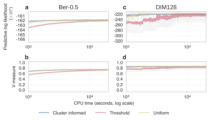
Next we compare the performance of different proposal distributions for the anchor auxiliary variables (Figures 3 c and d). For this experiment we kept the number of particles fixed at 20 and the resampling threshold at 0.5. We consider three proposal distributions.

Uniform:

Sample the anchors uniformly at random from the $\binom{{T}}{2}$ possibilities.

Cluster informed:

Sample the first anchor uniformly at random. Sample a cluster to draw the second anchor from with probability $\frac{1}{|c-1|}$ for the cluster containing the first anchor; otherwise proportional to

$$\frac{L(y_{\bar{b}\cup b})}{L(y_{\bar{b}})L(y_{b})}$$

where $\bar{b}$ is the cluster containing the first anchor and $b$ is the candidate cluster. Sample the second anchor uniformly from the chosen cluster.

Threshold informed:

Sample the first anchor uniformly at random and the second anchor from clusters that have Chinese restaurant attachment probabilities greater than a threshold of 0.01.

To ensure the adaptation of the informed proposals stops, and does not perturb the invariant distribution of the sampler, we only update the proposal distributions when the number of clusters instantiated breaks the previous record. Adaptation is guaranteed to terminate in finite time given there are only a finite number of points. This would usually take a long time, so in practice it is advantageous to stop adaptation after a fixed period of time. Detailed implementations of the cluster informed and threshold informed proposals are given in Appendix F. Our results suggest that performance is not strongly affected by the anchor proposal distribution ${h}$. We only saw a small advantage when using the informed proposal distributions for the auxiliary anchor variables in ${s}$. We also explored the effect of $h$ in higher dimensional datasets (Figure 4). Again we found the results are not sensitive to the choice of $h$. With the exception of the circle dataset, where we used the uniform proposal, we used the cluster informed prior for both the PGSM and SAMS samplers in subsequent experiments.

The frequency of the resampling step had a larger effect. A critical implementation point in order for the PGSM method to work is that resampling should be done adaptively by monitoring the ESS of the particle approximations in Algorithm 3 (Liu and Chen, 1995; Lee, 2011). We varied the relative ESS resampling threshold ${\beta}$ from 0 (never resample) to 1 (always resample) (Figures 3 e and f). We observed that the performance is markedly degraded if resampling is performed after each SMC iteration, but similar for all other resampling thresholds. We used a threshold of 0.5 in all other experiments.

Next, we used the dataset C1 to investigate the effectiveness of our method with the finite clustering model introduced in Section 2, with the number of clusters fixed to ${{k}_{0}}=5$. In this case, standard split-merge methods such as SAMS are less helpful since only merging can be performed when the maximum number of clusters has been allocated. The PGSM sampler does not have this restriction and naturally allows simultaneously splitting and merging while preserving the total number of clusters. Furthermore, the PGSM sampler can use more than two anchors, potentially allowing for large changes in configuration without altering the number of clusters. We compared the PGSM with two ($|s|=2$) and three ($|s|=3$) anchors to the Gibbs sampler. The PGSM method outperformed the Gibbs sampler, though increasing the number of anchors did not improve the performance (Figure 5 a). We plot the predictive densities (Figure 5 b, d, f) and cluster allocations (Figure 5 c, e, g) after running each sampler for 1000 seconds. At this point the PGSM sampler used a single cluster to model the points in the middle, while the Gibbs samplers used two clusters to model the central cluster.

In Figures 6 and 7 we show a series of experiments on the four datasets S1–4 describe in the previous section. We compare the PGSM to standard Gibbs and the SAMS method of Dahl (2003). We first compared pure kernels, where the split-merge samplers are not mixed with standard Gibbs moves (Figure 6). The pure PGSM kernel outperformed both Gibbs and SAMS on datasets S1 and S2. The Gibbs kernel and PGSM perform similarly for datasets S3 and S4, and both outperformed SAMS. When the split-merge moves are mixed with standard Gibbs moves, the split-merge methods outperformed Gibbs on datasets S1 and S2, with all methods showing similar performance on datasets S3 and S4 (Figure 7).

Finally, we explored the performance of the methods on four high dimensional datasets. The mixed PGSM and Gibbs samplers performed the best on the Bernoulli datasets, while the unmixed PGSM sampler is slower to reach the same predictive likelihood and V-measure (Figures 8 a-d). The mixed SAMS sampler failed to reach the same predictive likelihood as the PGSM and Gibbs methods, oscillating around lower values. The unmixed SAMS sampler appears to be trapped in a local mode, corresponding to poor predictive likelihood and V-measure. For the Normal datasets, the Gibbs sampler was trapped in a local mode and had markedly worse performance than other methods (Figures 8 e-h). The unmixed samplers outperformed the mixed equivalents on the 64 dimensional data. Furthermore, the unmixed PGSM method had a large performance advantage over all other methods on the 128 dimensional dataset.

We compared the performance of the three sampling methods on a geolocation dataset. The dataset, described in more detail in Fränti et al. (2010), consists of a subset of data collected by MOPSI, a Finnish mobile application where users can post their current geographic location via their mobile device. The subset we used consists of a list of 13,467 locations (latitude-longitude pairs) from users located in Finland until 2012. The data is freely accessible from http://cs.joensuu.fi/sipu/datasets/.

We use this data as a proxy for the estimation of mobile device user density. The DP mixture of Normal-Inverse-Wishart distributions provides a natural way to obtain a parsimonious estimate of population density, where the flexibility on the shape and number of clusters can accommodate a broad range of density variability factors ranging from densely populated cities to vast low-density rural areas.

We summarize the results in Figure 9. In Figures 9 a-c, we display quantitative results as measured by held-out predictive likelihood performance. In Figure 9 a, we show that mixed PGSM, mixed SAMS and Gibbs samplers perform similarly. In Figure 9 b, we show that the performance of SAMS is considerably degraded if SAMS is not mixed with a Gibbs kernel. In Figure 9 c, we show that the performance of PGSM is less degraded if not mixed with a Gibbs kernel.

In Figures 9 e-j, we visualize the posterior predictive density approximated using MCMC samples. We also show the raw data in Figure 9 d for reference. The following three pairs of density plots are included to illustrate the high computational cost of initializing a standard Gibbs sampler at a fully disconnected configuration. From left to right: the first pair shows the predictive density after one round of Gibbs sampling initialized at the fully disconnected configuration (Figures e and f); the second pair, after sampling with PGSM initialized at the fully connected configuration for the same time (Figures g and h); the third, after running the Gibbs sampler for $10^{5}$ seconds (Figures i and j). This demonstrates that our method can produce accurate and compact density estimates without relying on an expensive initialization phase.

The PyClone model (Roth et al., 2014) is designed to infer the proportion of cancer cells in a tumour sample which contain a mutation, which we refer to as the cellular prevalence of the mutation. The input data consists of a set of digital measurements of allelic abundance which is assumed to be proportional to the true abundance of the allele in the sample. The key factors which need to be deconvolved to convert this measurement to an estimate of cellular prevalence are that some cells derive from healthy (normal) tissue and the genomes of cancer cells contain multiple copies of a locus. The model assumes that mutations will group by cellular prevalence due to the expansion of populations of genetically identical cells. The number of populations is unknown, thus the PyClone model uses a DP prior with a Uniform($\left[0,1\right]$) base measure. The component parameters are interpreted as the cellular prevalence of the mutations associated with the component.

We show results on a dataset with 10,000 synthetic mutations in Figure 10. All methods except the pure SAMS kernel performed similarly in terms of predictive likelihood, while the pure SAMS kernel performed significantly worse (Figure 10 a). The pure PGSM and SAMS kernels outperformed the other methods in terms of V-measure, though the difference were small (Figures 10 b).

As observed in the other domains, the performance of SAMS critically depends on mixing the kernel with GIBBS moves. We show the data points for each replication of the pure split-merge kernels further supporting this point (Figure 10 c).

References

- Andrieu et al. (2009) C. Andrieu, A. Doucet, and R. Holenstein. Particle Markov chain Monte Carlo for efficient numerical simulation. In Monte Carlo and Quasi Monte Carlo Methods Conference 2008, Lecture Notes in Statistics, pages 45–60. Springer-Verlag, 2009.
- Andrieu et al. (2010) C. Andrieu, A. Doucet, and R. Holenstein. Particle Markov chain Monte Carlo methods. Journal of the Royal Statistical Society: Series B, 72(3):269–342, 2010.
- Caron and Doucet (2009) F. Caron and A. Doucet. Bayesian nonparametric models on decomposable graphs. In Advances in Neural Information Processing Systems, pages 225–233. 2009.
- Carvalho et al. (2010) C. Carvalho, H. Lopes, N. Polson, and M. Taddy. Particle learning for general mixtures. Bayesian Analysis, 5(4):709–740, 12 2010.
- Chang and Fisher III (2013) J. Chang and J. W. Fisher III. Parallel sampling of Dirichlet process mixutre models using sub-clusters splits. In Advances in Neural Information Processing Systems, pages 620–628, 2013.
- Chopin and Singh (2015) N. Chopin and S. S. Singh. On particle Gibbs sampling. Bernoulli, 21(3):1855–1883, 2015.
- Dahl (2003) D. B. Dahl. An improved merge-split sampler for conjugate Dirichlet process mixture models. Technical Report 1086, University of Wisconsin–Madison, 2003.
- Dahl (2009) D. B. Dahl. Modal clustering in a univariate class of product partition models. Bayesian Analysis, 4(2):243–264, 2009.
- Daumé III (2007) H. Daumé III. Fast search for Dirichlet process mixture models. In Proceedings of the International Conference on Artificial Intelligence and Statistics, 2007.
- Del Moral et al. (2006) P. Del Moral, A. Doucet, and A. Jasra. Sequential Monte Carlo samplers. Journal of the Royal Statistical Society: Series B, 68(3):411–436, 2006.
- Doucet and Johansen (2011) A. Doucet and A. M. Johansen. A tutorial on particle filtering and smoothing: Fifteen years later. In Oxford Handbook of Nonlinear Filtering. Oxford University Press, 2011.
- Escobar and West (1995) M. D. Escobar and M. West. Bayesian density estimation and inference using mixtures. Journal of the American Statistical Association, 90(430):577–588, 1995.
- Fearnhead (2004) P. Fearnhead. Particle filters for mixture models with an unknown number of components. Statistics and Computing, 14:11–21, 2004.
- Fearnhead and Clifford (2003) P. Fearnhead and P. Clifford. On-line inference for hidden Markov models via particle filters. Journal of the Royal Statistical Society: Series B, 65(4):887–899, 2003.
- Fearnhead and Meligkotsidou (2007) P. Fearnhead and L. Meligkotsidou. Filtering methods for mixture models. Journal of Computational and Graphical Statistics, 16(3):586–607, 2007.
- Ferguson (1973) T. S. Ferguson. A Bayesian analysis of some nonparametric problems. The Annals of Statistics, 1(2):209–230, 1973.
- Franti and Virmajoki (2006) P. Franti and O. Virmajoki. Iterative shrinking method for clustering problems. Pattern Recognition, 39(5):761–765, 2006.
- Fränti et al. (2006) P. Fränti, O. Virmajoki, and V. Hautamäki. Fast agglomerative clustering using a k-nearest neighbor graph. IEEE Trans. on Pattern Analysis and Machine Intelligence, 28(11):1875–1881, 2006.
- Fränti et al. (2010) P. Fränti, J. Kuittinen, A. Tabarcea, and L. Sakala. MOPSI location-based search engine: concept, architecture and prototype. In ACM Symposium on Applied Computing, volume 10, pages 872–873, 2010.
- Gal and Ghahramani (2014) Y. Gal and Z. Ghahramani. Pitfalls in the use of parallel inference for the Dirichlet process. In Proceedings of the 31st International Conference on Machine Learning, pages 208–216. JMLR Workshop and Conference Proceedings, 2014.
- Ge et al. (2015) H. Ge, Y. Chen, M. Wan, and Z. Ghahramani. Distributed inference for Dirichlet process mixture models. In Proceedings of the 32nd International Conference on Machine Learning, pages 2276–2284, 2015.
- Ishwaran and James (2001) H. Ishwaran and L. F. James. Gibbs sampling methods for stick-breaking priors. Journal of the American Statistical Association, 96:161–173, 2001.
- Ishwaran and James (2003) H. Ishwaran and L. F. James. Generalized weighted Chinese restaurant processes for species sampling mixture models. Statistica Sinica, 13:1211–1235, 2003.
- Jain and Neal (2004) S. Jain and R. M. Neal. A split-merge Markov chain Monte Carlo procedure for the Dirichlet Process mixture model. Journal of Computational and Graphical Statistics, 13:158–182, 2004.
- Johansen (2009) A. M. Johansen. SMCTC: Sequential Monte Carlo in C++. Journal of Statistical Software, 30(6):1–41, 2009.
- Jun et al. (2012) S. Jun, L. Wang, and A. Bouchard-Côté. Entangled Monte Carlo. In Advances in Neural Information Processing Systems, volume 25, pages 2735–2743, 2012.
- Kalli et al. (2011) M. Kalli, J. E. Griffin, and S. G. Walker. Slice sampling mixture models. Statistics and Computing, 21(1):93–105, 2011.
- Kantas et al. (2015) N. Kantas, A. Doucet, S. S. Singh, J. M. Maciejowski, and N. Chopin. On particle methods for parameter estimation in state-space models. Statistical Science, 30(3):328–351, 2015.
- Lee (2011) A. Lee. On auxiliary variables and many-core architectures in computational statistics. PhD thesis, Department of Statistics, Oxford University, 2011.
- Lee and Whiteley (2016) A. Lee and N. Whiteley. Forest resampling for distributed sequential Monte Carlo. Statistical Analysis and Data Mining, 9(4):230–248, 2016.
- Lee et al. (2010) A. Lee, C. Yau, M. Giles, A. Doucet, and C. Holmes. On the utility of graphics cards to perform massively parallel simulation of advanced Monte Carlo methods. Journal of Computational and Graphical Statistics, 19(4):769–789, 2010.
- Liang et al. (2007) P. Liang, M. I. Jordan, and B. Taskar. A permutation-augmented sampler for Dirichlet process mixture models. Proceedings of the International Conference on Machine learning, 24:545–552, 2007.
- Lindsten et al. (2014) F. Lindsten, M. I. Jordan, and T. B. Schön. Particle Gibbs with ancestor sampling. Journal of Machine Learning Research, 15:2145–2184, 2014.
- Liu and Chen (1995) J.S. Liu and R. Chen. Blind deconvolution via sequential imputation. Journal of the American Statistical Association, 90:567–576, 1995.
- MacEachern (1994) S. N. MacEachern. Estimating normal means with a conjugate style Dirichlet process prior. Communications in Statistics: Simulation and Computation, 23:727–741, 1994.
- MacEachern et al. (1999) S. N. MacEachern, M. Clyde, and J. S. Liu. Sequential importance sampling for nonparametric Bayes models: The next generation. Canadian Journal of Statistics, 27(2):251–267, 1999.
- Mansinghka et al. (2007) V. K. Mansinghka, D. M. Roy, R. Rifkin, and J. Tenenbaum. AClass: An online algorithm for generative classification. In Proceedings of the 11th International Conference on Artificial Intelligence and Statistics, volume 2, pages 315–322, 2007.
- Marin et al. (2005) J. Marin, K. L. Mengersen, and C. Robert. Bayesian modelling and inference on mixtures of distributions. In D. Dey and C.R. Rao, editors, Handbook of Statistics: Volume 25. Elsevier, 2005.
- Murray et al. (2016) L. Murray, A. Lee, and P. Jacob. Parallel resampling in the particle filter. Journal of Computational and Graphical Statistics, 25(3):789–805, 2016.
- Murray (2015) L. M. Murray. Bayesian state-space modelling on high-performance hardware using LibBi. Journal of Statistical Software, 67(10):1–36, 2015.
- Neal (2000) R. M. Neal. Markov chain sampling methods for Dirichlet process mixture models. Journal of Computational and Graphical Statistics, 9:249–265, 2000.
- Pitman and Yor (1997) J. Pitman and M. Yor. The two-parameter Poisson-Dirichlet distribution derived from a stable subordinator. Annals of Probability, 25(2):855–900, 1997.
- Richardson and Green (1997) S. Richardson and P. J. Green. On Bayesian analysis of mixtures with an unknown number of components. Journal of the Royal Statistical Society: Series B, 59:731–792, 1997.
- Rosenberg and Hirschberg (2007) Andrew Rosenberg and Julia Hirschberg. V-measure: A conditional entropy-based external cluster evaluation measure. In EMNLP-CoNLL, volume 7, pages 410–420, 2007.
- Roth et al. (2014) A. Roth, J. Khattra, D. Yap, A. Wan, E. Laks, J. Biele, G. Ha, S. Aparicio, A. Bouchard-Côté, and S. P. Shah. PyClone: statistical inference of clonal population structure in cancer. Nature methods, 11(4):396–398, 2014.
- Sudderth (2006) E. B. Sudderth. Graphical Models for Visual Object Recognition and Tracking. PhD thesis, Massachusetts Institute of Technology, Cambridge, Massachusetts, 2006.
- Ülker et al. (2010) Y. Ülker, B. Günsel, and A. T. Cemgil. Sequential Monte Carlo samplers for Dirichlet process mixtures. In Proceedings of the 13th International Conference on Artificial Intelligence and Statistics, volume 9, pages 876–883, 2010.
- Walker (2007) S. G. Walker. Sampling the Dirichlet mixture model with slices. Communications in Statistics - Simulation and Computation, 36(1):45–54, 2007.
- Wang and Dunson (2011) L. Wang and D. B. Dunson. Fast Bayesian inference in Dirichlet process mixture models. Journal of Computational and Graphical Statistics, 20(1):196–216, 2011.
- Whiteley (2010) N. Whiteley. Discussion on Particle Markov chain Monte Carlo methods. Journal of the Royal Statistical Society: Series B, 72:306–307, 2010.
- Whiteley et al. (2010) N. Whiteley, C. Andrieu, and A. Doucet. Efficient Bayesian inference for switching state space models using discrete particle Markov chain Monte Carlo methods. Technical Report 10:04, Bristol Statistics Research Report, 2010.
- Williamson et al. (2013) S. Williamson, A. Dubey, and E. Xing. Parallel Markov chain Monte Carlo for nonparametric mixture models. In Proceedings of the 30th International Conference on Machine Learning, pages 98–106, 2013.