Perturbing open cavities: Anomalous resonance frequency shifts in a hybrid cavity-nanoantenna system

The fact that a small perturbation of a potential can influence the distribution of a system’s energy levels is a well-known principle permeating various branches of physics. In quantum mechanics, for example, the effect of a perturbing potential $H^{\prime}$ on an eigenstate $\ket{\psi_{0}}$ is that it modifies its unperturbed energy $U_{0}$ by an amount $\delta U=\braket{\psi_{0}|H^{\prime}|\psi}$, where $\ket{\psi}$ is the new eigenstate and we assume $\braket{\psi_{0}|\psi}\approx 1$. In electrodynamics, a local change of potential (i.e. permittivity) can impact the frequency of a resonant cavity. This is at the basis of many applications that use the influence of a perturbing atom, molecule, or dielectric body to establish an interaction that can be exploited for optical sensing or control [1, 2, 3, 4, 5, 6, 7, 8]. The shift of a mode’s complex eigenfrequency $\omega=\omega_{\mathrm{c}}-\mathrm{i}\kappa/2$, with cavity resonance frequency $\omega_{\mathrm{c}}$ and linewidth $\kappa$, due to a local permittivity perturbation $\Delta\epsilon$ contained in a volume $\Delta V$ is given by $\delta\omega/\omega=-\int_{\Delta V}dV\left[\epsilon_{0}\Delta\epsilon\mathbf{E}_{0}^{\ast}\cdot\mathbf{E}_{p}\right]/4U_{0}$. Here $\mathbf{E}_{0}$ and $U_{0}$ represent the field and total energy of the unperturbed cavity mode, respectively, and $\mathbf{E}_{p}$ is the perturbed field [9, 10]. In particular, if $\Delta V$ is small enough such that the perturbing particle can be described in the dipole approximation, the complex frequency shift is directly related to the particle polarizability $\alpha$, reading $\delta\omega/\omega=-\alpha|\mathbf{E}_{0}|^{2}/4U_{0}$ [9]. However, this widely employed result of Bethe-Schwinger perturbation theory [10] is strictly only valid when radiation to the far field is negligible. In several recent developments, radiation loss proved decisive in determining a system’s eigenmode, e.g. for so-called ‘states bound in the continuum’ [11, 12, 13] and in describing complex plasmonic resonators [14, 15]. In that context, the question arises to what extent the conventional paradigm to determine perturbed cavity frequencies holds in practical, open, systems.

Here, we study the eigenfrequencies of a radiating optical cavity as it is perturbed by carefully designed resonant plasmonic nanoparticles. For a resonant perturbation with center frequency $\omega_{\mathrm{a}}$ and linewidth $\gamma$, the value of $\alpha$ strongly depends on the detuning $\Delta=\omega_{\mathrm{c}}-\omega_{\mathrm{a}}$. In absence of radiation, the cavity mode thus redshifts(blueshifts) at negative(positive) values of $\Delta$ and the linewidth broadens near $\Delta=0$, in direct response to Re[$\alpha$] and Im[$\alpha$], respectively (Fig 1a). Tuning $\omega_{\mathrm{a}}$ by varying the length of the (plasmonic) resonators allows to systematically study the induced cavity response as a function of detuning. Importantly, our experiment is designed such that radiation losses from the cavity mode and plasmonic resonators overlap. This, as we will show, leads to a strong additional contribution to $\delta\omega$ which is not captured by $\alpha$. We study this ‘radiation interaction’, as we will call the effect, in detail and show that it can induce strong eigenfrequency shifts that are opposite to, and even exceed, the effects based on the particles’ polarizability.

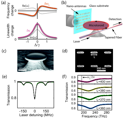
A sketch of the system is shown in Fig. 1b. The experiments are performed using a fundamental cavity mode (194.4 THz, Q$\sim$6.5$\times 10^{6}$, TE polarized) of a toroidal silica microcavity fabricated on the edge of a silicon chip ($\approx$36 $\mu$m diameter, Fig. 1c) [16, 17]. The cavity is perturbed by gold nanoantennas deposited on a glass substrate (Fig. 1d), which are controllably placed in the evanescent field of the cavity. The antennas (nanorods of length $L$, width 120 nm and thickness 40 nm) are aligned with their (long) principal dipole axis to the polarization of the cavity mode. A frequency-swept narrowband laser source ($\sim$0.7 $\mu$W) is coupled into a tapered fiber that is brought close to the cavity. The transmission spectrum through the fiber shows a Lorentzian dip around the cavity resonance frequency (Fig. 1e), from which we determine the (perturbed) resonance frequency $\omega_{\mathrm{c}}$ and linewidth $\kappa$ of the cavity mode. Independent normal-incidence transmission measurements (Fig. 1f) on the fabricated antenna arrays, in absence of the cavity, yield the normalized cavity-antenna detuning $\Delta/\gamma$. Notably, the presence of the glass substrate allows the cavity mode to radiate into the glass at a well defined angle just beyond the critical angle and, similarly, allows scattering of antenna radiation into the substrate [18]. As the antennas are coherently excited by the cavity field, from which also the cavity radiation originates, the zeroth-order diffraction by the array is expected to overlap with the cavity radiation.

To measure the change of the complex cavity resonance frequency due to the nanoantennas, we compare the frequency and linewidth of the cavity mode with and without the antenna array placed in the near-field of the cavity. Our measurement procedure [19] ensures that in both cases the sample is positioned at the same distance to the cavity. Figure 2a shows the results for two different arrays of nanoantennas: In the top figure, an antenna array ($L=360$, pitch 800(900) nm along the long(short) axes of the antennas) is seen to induce a broadening of the cavity linewidth, together with a blueshift of the frequency. The latter is clearly surprising, given the fact that $\Delta\approx-1.2\gamma$ for this sample [19], where one expects a redshift if one only considers the resonant particle’s polarizability (Fig. 1a). The bottom panel in Fig. 2a shows that for another array ($L=400$, pitch 800(1100) nm) with slightly positive detuning ($\Delta\approx 0.8\gamma$) again a blueshift is observed, but this time accompanied by narrowing of the cavity mode. Such a reduction of damping can obviously not be ascribed to the particle’s polarizability alone, as its imaginary part is necessarily positive (Fig. 1a).

To systematically study these effects, we gradually tune the resonance frequency $\omega_{a}$ by varying the length of the antennas (Fig. 1f). The array pitch is kept fixed at 800(1500) nm along the long(short) antenna axes, chosen such that inter-antenna coupling is negligible. Moreover, in all examples we show, Bragg-scattering between clockwise and counter-clockwise modes [20] is small enough such that mode splitting induced by the nanoantennas is smaller than the cavity linewidth. Figure 2b shows the resulting cavity frequency and linewidth changes, normalized to the cavity linewidth on glass to allow averaging multiple scans [19], as a function of $\Delta/\gamma$. For these negative detunings, a consistent increase of the resonance frequency (i.e. blueshift) is observed that slightly rises as the antenna frequency approaches that of the cavity. As such, both the sign and the trend of $\delta\omega_{\mathrm{c}}$ are incongruous with the expectation based on the polarizability (Fig. 1a). Moreover, the broadening of the cavity, observed for a detuning of $\Delta\approx-0.6\gamma$, quickly reduces as the – strongly scattering – antennas are tuned closer to the cavity resonance. We note that these trends are consistently observed also at other periodicities [19] and that the shifts cannot be explained by thermal heating, negligible at the employed powers.

To explore the origin of these surprising results, it is necessary to consider the complete Bethe-Schwinger cavity perturbation equation [10], derived without neglecting radiation:

This full expression, which is also valid in any open, non-Hermitian system [19], contains an additional integral term involving radiated fields at a surface $\delta V$ (with normal unit vector $\mathbf{\hat{n}}$), enclosing the same volume that was used to evaluate the total energy $U_{0}$. Here, $\delta\mathbf{E}$ and $\delta\mathbf{H}$ are the difference between the fields in the presence ($\mathbf{E}_{p}$, $\mathbf{H}_{p}$) and absence ($\mathbf{E}_{0}$, $\mathbf{H}_{0}$) of the perturbation, and can as such be associated with the field scattered by the perturbation. Thus, the cavity eigenfrequency is additionally modified by an energy flux that is evaluated by combining the fields of the perturbed and unperturbed eigenmodes; i.e, an overlap of scattering by the perturbation and direct cavity radiation. Remarkably, the integral is independent of the distance at which $\delta V$ is chosen, consistent with the fact that it can be associated with radiation of the system. To date, this far-field contribution has been omitted in practically all analyses of cavity perturbation. In a select number of experiments, a reduction of cavity linewidth was observed [21, 22, 23] and tentatively attributed to interference of radiation of the cavity and scattering by the perturbation. Importantly, the integral suggests that in principle also the resonance frequency (i.e., the real part of $\delta\omega$) can be affected by the same mechanism, if the phase difference between cavity and scattered radiation in the far field (captured in $\mathbf{E}_{0}$ and $\delta\mathbf{E}$, respectively) differs from 0 or $\pi$. So far, the frequency has been expected to rely only on the local variation of the applied potential [24, 25, 23, 26, 3, 18] as it is contained in the first term of (1).

To verify the importance of radiation in a complete description of the induced cavity response, we perform finite-element method eigenfrequency studies with and without antenna [19] in a similar two-dimensional system (Fig. 3a), from which we extract the fields $\mathbf{E}_{0}$, $\mathbf{H}_{0}$, $\delta\mathbf{E}$ and $\delta\mathbf{H}$. This allows the calculation of the individual terms of (1), displayed as a function of detuning in Fig. 3b. The first term (black crosses, ‘A’), contributes to $\delta\omega$ according to the expected behaviour for a perturbing resonator sketched in Fig. 1a: it produces a dispersive detuning dependence of $\delta\omega_{\mathrm{c}}$ and a dissipative trend for $\delta\kappa$. This immediately disqualifies this term as an explanation for the measured changes in cavity resonance and linewidth. The second term, i.e. the contribution to the change in eigenfrequency related to the radiation interaction (green stars, ‘B’), shows a dramatically different behavior: it causes distinct blueshifts and linewidth narrowing around $\Delta/\gamma=0$. Surprisingly, the magnitude of the blueshifts induced by this term can even exceed the contribution due to $\alpha$. This is a key point of our observation, stressing the importance of this new contribution in a model system. The sum of both terms (blue circles, A+B) yields the complete eigenfrequency shift of the perturbed cavity, which now qualitatively matches our experimental results; blueshifts and linewidth narrowing around $\Delta/\gamma=0$. These calculations thus confirm that radiation interactions in open systems can lead to both cavity blueshifts and linewidth narrowing and importantly, that this effect can even dominate the total change in eigenfrequency of a cavity mode.

It is essential to realize that a modification of the cavity resonance frequency (in contrast to the alteration of the linewidth) due to back-action via the radiation continuum only occurs when the phase $\delta\phi$ between cavity and antenna radiation is different from 0 or $\pi$ (Fig. 4a). The exact strength of this back-action, and as such the sum of direct (i.e. due to $\alpha$) and indirect (i.e. via the radiation continuum) coupling between cavity and antenna, will depend on the overlap between their radiation profiles and on the value of $\delta\phi$.

This phase difference and its physical connection to back-action can be captured in a simple model (Fig. 4b) based on temporal coupled-mode theory [27]. Let us assume for now that the cavity and antenna are coupled with complex coupling rate $\tilde{g}_{\mathrm{c}}=g_{\mathrm{c}}\,e^{\mathrm{i}\phi_{\mathrm{c}}}$ and can both interact with the environment (glass) with coupling rates $\tilde{g}_{\kappa}=g_{\kappa}\,e^{\mathrm{i}\phi_{\kappa}}$ and $\tilde{g}_{\gamma}=g_{\mathrm{\gamma}}\,e^{\mathrm{i}\phi_{\gamma}}$, respectively. We treat the joint environment as a separate mode to allow backaction, taking the limit of large decay rate $\zeta$ to mimic a broadband continuum. The cavity and antenna, considered separately, each decay via this continuum at a rate $\kappa_{1}=4|g_{\kappa}|^{2}/\zeta$ and $\gamma_{1}=4|g_{\mathrm{\gamma}}|^{2}/\zeta$, respectively. This is distinguished from decay into all other, non-overlapping, modes at rates $\kappa_{\mathrm{0}}$ and $\gamma_{\mathrm{0}}$, such that $\kappa_{\mathrm{0}}+\kappa_{1}=\kappa$ and $\gamma_{\mathrm{0}}+\gamma_{1}=\gamma$. Importantly, the phase difference between cavity radiation (blue path, Fig. 4b) and antenna scattering (orange path, Fig. 4b) in this model now directly relates to $\delta\phi$ via $\delta\phi=\pi+\Phi-\text{arg}[\Delta+\mathrm{i}\gamma/2]$, where $\Phi=\phi_{\mathrm{c}}+\phi_{\kappa}+\phi_{\gamma}$, and $\text{arg}[\Delta+\mathrm{i}\gamma/2]$ is the phase response of the antennas [19]. The natural mode of interest, with complex frequency $\omega$, of this hybrid system can be found by equating the determinant of the coupling matrix [19]

to zero. Solving for complex $\omega$ yields

which depends on the radiation overlap $\kappa_{1}\gamma_{1}$, (constant) phase $\Phi$ and the coupling rate $g_{\mathrm{c}}$. Because the overlap and phase $\Phi$ cannot be independently chosen, it is impossible to directly fit (3) to the experimental data. Therefore, we retrieve $\delta\phi$ from the finite element simulation and, using the relation between $\delta\phi$ and $\Phi$, obtain $\Phi=3.76\times 10^{-4}\pi$. Note that this value of $\Phi$ implies that $\delta\phi\approx\pi/2$ at $\Delta=0$, completely opposite to the conventionally assumed case where destructive interference ($\delta\phi=\pi$) only contributes to the linewidth of the cavity mode. Fixing $\Phi$ at this value and constraining the experimentally found values of $\kappa$, $\Delta$ and $\gamma$ (retrieved from independent spectroscopic measurements, Fig. 1), a fit of (3) yields excellent correspondence to our data in Fig. 2b (solid lines), resulting in an overlap of $\kappa_{1}\gamma_{1}/\kappa\gamma=0.68$ and coupling rate $g_{\mathrm{c}}/2\pi=21.6$ GHz.

Concluding, we have shown how coupling through the radiation continuum leads to cavity blueshifts and linewidth narrowing in a coupled cavity-antenna system. Surprisingly, the non-local, radiative effect on the cavity is larger than the induced cavity response due to local perturbations, and is not just an artefact of large radiation losses but can even manifest itself in a high-Q cavity such as studied here. Therefore, similar effects are expected in many other systems where cavity and perturbation can radiate into the same channels, such as photonic crystals [21, 22, 23, 28] and Fabry-Pérot etalons [29, 30, 31]. In addition, it was shown that there is a direct link between the phase $\delta\phi$ in the Bethe-Schwinger equation and the contributions to back-action in a coupled-mode model.

Interestingly, these results could also shed new light on radiative interactions in strongly radiating systems such as metamaterials and complex plasmonic resonators. In [14], it was postulated that radiation can be included in the coupling between two resonators by using a complex coupling rate, while in [32], a complex coupling rate was argued to originate from a complex-valued extinction cross-section. In fact, such a complex coupling rate between two resonators is easily derived from the coupled-mode model presented in this work [19]. Furthermore, it will be interesting to see how the concepts and theory established here relate to recently developed methods to relying on the normalization of leaky modes to describe the response of complex photonic systems [33, 34]. In a different context, recent advances in optomechanics using simultaneous dispersive and dissipative (i.e radiative) coupling [35, 36, 37] have been reported to enable on-resonance cooling [35] and sensitive readout of nanomechanical motion [36]. As such, we expect our work to be directly important to the design of novel optical devices such as sensors, for example, and benefit the understanding of the physics of open systems in optics and beyond.

This work is part of the research programme of the Foundation for Fundamental Research on Matter (FOM), which is part of the Netherlands Organisation for Scientic Research (NWO). EV gratefully acknowledges support from an NWO Vidi grant.

Supplementary Material

References

- [1] J. M. Raimond, M. Brune, and S. Haroche, Rev. Mod. Phys. 73, 565 (2001).
- [2] P. Lodahl, S. Mahmoodian, and S. Stobbe, Rev. Mod. Phys. 87, 347 (2015).
- [3] F. Vollmer and S. Arnold, Nat. Methods 5, 591 (2008).
- [4] X. Fan, I. M. White, S. I. Shopova, H. Zhu, J. D. Suter, and Y. Sun, Anal. Chim. Acta 620, 8 (2008).
- [5] M. Aspelmeyer, T. J. Kippenberg, and F. Marquardt, Rev. Mod. Phys. 86, 1391 (2014).
- [6] J. Zhu, S. K. Ozdemir, Y.-F. Xiao, L. Li, L. He, D.-R. Chen, and L. Yang, Nat. Photonics 4, 46 (2010).
- [7] J. D. Thompson, T. G. Tiecke, N. P. de Leon, J. Feist, A. V. Akimov, M. Gullans, A. S. Zibrov, V. Vuletić, and M. D. Lukin, Science 340, 1202 (2013).
- [8] A. Goban, C.-L. Hung, S.-P. Yu, J. D. Hood, J. A. Muniz, J. H. Lee, M. J. Martin, A. C. McClung, K. S. Choi, D. E. Chang, O. Painter, and H. J. Kimble, Nat. Commun. 5, 3808 (2014).
- [9] R. A. Waldron, Proc. IEE Part C Monogr. 107, 272 (1960).
- [10] H. A. Bethe and J. Schwinger, Perturbation theory for cavities (Massachusetts Institute of Technology, Radiation Laboratory, Cambridge, 1943).
- [11] H. Friedrich and D. Wintgen, Phys. Rev. A 32, 3231 (1985).
- [12] C. W. Hsu, B. Zhen, J. Lee, S.-L. Chua, S. G. Johnson, J. D. Joannopoulos, and M. Soljačić, Nature 499, 188 (2013).
- [13] F. Monticone and A. Alù, Phys. Rev. Lett. 112, 213903 (2014).
- [14] R. Taubert, M. Hentschel, J. Kästel, and H. Giessen, Nano Lett. 12, 1367 (2012).
- [15] N. Liu, L. Langguth, T. Weiss, J. Kästel, M. Fleischhauer, T. Pfau, and H. Giessen, Nat. Mater. 8, 758 (2009).
- [16] D. K. Armani, T. J. Kippenberg, S. M. Spillane, and K. J. Vahala, Nature 421, 925 (2003).
- [17] G. Anetsberger, O. Arcizet, Q. P. Unterreithmeier, R. Rivière, A. Schliesser, E. M. Weig, J. P. Kotthaus, and T. J. Kippenberg, Nat. Phys. 5, 909 (2009).
- [18] L. Novotny and B. Hecht, Principles of Nano-Optics (Cambridge University Press, Cambridge, 2012).
- [19] See Supplemental Material for detailed information about our measurement procedure, experimental setup and results for antenna arrays with different pitches, as well as details regarding the finite-element simulation and derivations of equations (1-3).
- [20] A. Mazzei, S. Götzinger, L. de S. Menezes, G. Zumofen, O. Benson, and V. Sandoghdar, Phys. Rev. Lett. 99, 173603 (2007).
- [21] A. F. Koenderink, M. Kafesaki, B. C. Buchler, and V. Sandoghdar, Phys. Rev. Lett. 95, 153904 (2005).
- [22] J. T. Robinson and M. Lipson, Phys. Rev. Lett. 100, 043902 (2008).
- [23] M. Burresi, T. Kampfrath, D. van Oosten, J. C. Prangsma, B. S. Song, S. Noda, and L. Kuipers, Phys. Rev. Lett. 105, 123901 (2010).
- [24] S. Vignolini, F. Intonti, F. Riboli, L. Balet, L. H. Li, M. Francardi, A. Gerardino, A. Fiore, D. S. Wiersma, and M. Gurioli, Phys. Rev. Lett. 105, 123902 (2010).
- [25] L. Lalouat, B. Cluzel, P. Velha, E. Picard, D. Peyrade, J. P. Hugonin, P. Lalanne, E. Hadji, and F. de Fornel, Phys. Rev. B 76, 041102 (2007).
- [26] S. Arnold, M. Khoshsima, I. Teraoka, S. Holler, and F. Vollmer, Opt. Lett. 28, 272 (2003).
- [27] W. Suh, Z. Wang, and S. Fan, IEEE J. Quant. Electron. 40, 1511 (2004).
- [28] M. Barth, S. Schietinger, S. Fischer, J. Becker, N. Nüsse, T. Aichele, B. Löchel, C. Sönnichsen, and O. Benson, Nano Lett. 10, 891 (2010).
- [29] A. Mitra, H. Harutyunyan, S. Palomba, and L. Novotny, Opt. Lett. 35, 953 (2010).
- [30] D. Chanda, K. Shigeta, T. Truong, E. Lui, A. Mihi, M. Schulmerich, P. V. Braun, R. Bhargava, and J. A. Rogers, Nat. Commun. 2, 479 (2011).
- [31] R. Ameling and H. Giessen, Laser Photon. Rev. 7, 141 (2013).
- [32] S. Bakhti, N. Destouches, and A. V. Tishchenko, ACS Photonics 2, 246 (2015).
- [33] C. Sauvan, J. P. Hugonin, I. S. Maksymov, and P. Lalanne, Phys. Rev. Lett. 110, 237401 (2013).
- [34] J. Yang, H. Giessen, and P. Lalanne, Nano Lett. 15, 3439 (2015).
- [35] A. Sawadsky, H. Kaufer, R. M. Nia, S. P. Tarabrin, F. Y. Khalili, K. Hammerer, and R. Schnabel, Phys. Rev. Lett. 114, 043601 (2015).
- [36] A. C. Hryciw, M. Wu, B. Khanaliloo, and P. E. Barclay, Optica 2, 491 (2015).
- [37] A. Xuereb, R. Schnabel, and K. Hammerer, Phys. Rev. Lett. 107, 213604 (2011).
- [1] R. A. Waldron, Proc. IEE Part C Monogr. 107, 272 (1960).
- [2] H. A. Bethe and J. Schwinger, Perturbation theory for cavities (Massachusetts Institute of Technology, Radiation Laboratory, Cambridge, 1943).
- [3] Due to the different (engineering) convention used in COMSOL, implementation of this formula requires to switch the sign in front of the surface integral from (-) to (+).
- [4] D. K. Armani, T. J. Kippenberg, S. M. Spillane, and K. J. Vahala, Nature 421, 925 (2003).
- [5] G. Anetsberger, O. Arcizet, Q. P. Unterreithmeier, R. Rivière, A. Schliesser, E. M. Weig, J. P. Kotthaus, and T. J. Kippenberg, Nat. Phys. 5, 909 (2009).
- [6] L. Novotny and B. Hecht, Principles of Nano-Optics (Cambridge University Press, Cambridge, 2012).
- [7] COMSOL personal communication.
- [8] W. Suh, Z. Wang, and S. Fan, IEEE J. Quant. Electron. 40, 1511 (2004).
- [9] Due to the different (engineering) convention used in COMSOL, implementation of this formula requires to place a (-) sign in front of the right-hand side of expression (S39) when analyzing COMSOL data.
- [10] F. J. García de Abajo, Rev. Mod. Phys. 79, 1267 (2007).