Quantum phase transitions and Berezinskii-Kosterlitz-Thouless temperature
in a two-dimensional spin-orbit-coupled Fermi gas

In this work, we use a functional-integral approach to calculate thermodynamic properties of the system. More specifically, we write the partition function as a sum over Grassmann fields $\bar{\psi}$ and $\psi$, weighted by the exponential of the action functional $S$

Here, $\textbf{r}=(x,y)$ and $\tau$ indicate position and imaginary time, respectively, while $s=\{\uparrow,\downarrow\}$ denotes the spin-state (spin-up and spin-down) of the spin-1/2 fermions. The action can be related to the Hamiltonian density $\mathcal{H}$ via a Legendre transformation

Our aim is to study a two-dimensional (2D) Fermi gas, where the spin-orbit coupling is a generic combination of Rashba and Dresselhaus terms. The Hamiltonian density of this system can be divided into three parts: $\mathcal{H}=\mathcal{H}_{\rm{0}}+\mathcal{H}_{\rm{S}}+\mathcal{H}_{\rm{I}}$. Note that for the remainder of this paper we use the units $\hbar=2m=k_{\rm{F}}=1$.
The first part of $\mathcal{H}$ is

corresponding to the single-particle sector. We work in the grand canonical ensemble, hence the use of the Lagrange multiplier $\mu_{s}$, which is interpreted as a spin-dependent chemical potential, thus allowing for population imbalance. Furthermore, $h_{z}$ denotes a Zeeman field perpendicular to the (x-y)-plane. Experimentally, this field corresponds to the intensity $\Omega$ of the Raman transition between different hyperfine states: $h_{z}=-\Omega/2$. Finally, $\sigma_{i}$ represents the $i^{th}$ Pauli matrix.
The second part of $\mathcal{H}$ is

corresponding to the spin-orbit terms. Here, we have defined $\alpha=(v_{\rm{R}}+v_{\rm{D}})/2$ and $\gamma=(v_{\rm{R}}-v_{\rm{D}})/2$, with $v_{\rm{R}}$ and $v_{\rm{D}}$ being the Rashba and Dresselhaus coupling strength, respectively. Moreover, $\hat{k}_{l}=-i(\partial/\partial l)$ is the momentum operator along the $l$-direction.
The third part $\mathcal{H}_{\rm{I}}$ describes the interaction between fermions. We consider s-wave scattering, thus only taking into account interaction between fermions in different spin states. For a general two-body potential $V(\textbf{r}-\textbf{r}^{\prime})$, the interaction term can be written as

However, in this work, we restrict ourselves to short-range interactions, which can be described by the contact potential $V(\textbf{r}-\textbf{r}^{\prime})=g\delta(\textbf{r}-\textbf{r}^{\prime})$.
Having set up the functional-integral formalism, we are ready to discuss the saddle-point approximation.

The Hamiltonian density of the system has four eigenvalues: two quasiparticle energies $\epsilon_{\rm{p}}^{(\pm)}(\textbf{k})$, shown in Eq. (16), and two quasihole energies $\epsilon_{\rm{h}}^{(\pm)}(\textbf{k})=-\epsilon_{\rm{p}}^{(\pm)}(\textbf{k})$. The structure of these excitation spectra can be used to distinguish different uniform superfluid (US) phases. Let us look more closely at the quasiparticle branches. The (+)-branch is always gapped, whereas the (-)-branch can have nodes depending on the system parameters. In the language of the generalized helicity basis, we can write the second quasiparticle energy as

Here, we have introduced the energy associated with the singlet channel $E_{\rm{S}}(\textbf{k})=\sqrt{\xi_{\textbf{k}}^{2}+|\widetilde{\Delta}_{\rm{S}}(\textbf{k})|^{2}}$, as well as an effective magnetic field $\textbf{h}_{\rm{eff}}(\textbf{k})=(h_{\bot}(\textbf{k}),h_{z})$ which is a combination of the spin-orbit and the Zeeman fields. This effective field can also be written as half the energy difference of the generalized helicity bands $|\textbf{h}_{\rm{eff}}|=[\xi_{\Downarrow}(\textbf{k})-\xi_{\Uparrow}(\textbf{k})]/2$, while the single-particle energy is equal to the average energy of the helicity bands $\xi_{\textbf{k}}=[\xi_{\Uparrow}(\textbf{k})+\xi_{\Downarrow}(\textbf{k})]/2$.
The lowest quasiparticle energy branch $\epsilon_{\rm{p}}^{(-)}(\textbf{k})$ has nodes whenever the following two conditions are satisfied simultaneously: 1) the effective magnetic field $\textbf{h}_{\rm{eff}}(\textbf{k})$ and the singlet energy $E_{\rm{S}}(\textbf{k})$ are equal in magnitude, and 2) the triplet component $\widetilde{\Delta}_{\rm{T}}(\textbf{k})$ of the order parameter is zero. In the ERD case, $\widetilde{\Delta}_{\rm{T}}(\textbf{k})=0$ leads to $k_{x}=0$, which together with $E_{\rm{S}}(\textbf{k})=|h_{\rm{eff}}(\textbf{k})|$ gives the relation $(k_{y}^{2}-\mu)^{2}+|\Delta|^{2}=h_{z}^{2}$, yielding the possibility of having nodes at non-zero momentum. By contrast, in the RO case, or any other combination of Rashba and Dresselhaus terms, no nodes are present at non-zero momentum.
The different possible phases in the ERD case are shown in Fig. 1. Let us describe these phases in more detail. When the Zeeman field is smaller than the order parameter ($h_{z}<|\Delta|$), two phases can be discerned: 1) If the chemical potential $\mu>0$, the system acquires an indirect gap at non-zero $|\Delta|$, and 2) if $\mu<0$ a direct gap at $k_{y}=0$ occurs. These phases are labeled i-US-0 and d-US-0, respectively. When the Zeeman field becomes larger than the order parameter ($h_{z}>|\Delta|$), the quasiparticle spectrum acquires a nodal structure, depending on the value of the chemical potential. If $\mu>\sqrt{h_{z}^{2}-|\Delta|^{2}}$, the spectrum has two pairs of nodes (US-2 phase). When $|\mu|<\sqrt{h_{z}^{2}-|\Delta|^{2}}$, one pair of nodes is removed from the spectrum at $k=0$ and only one pair remains (US-1 phase). Finally, when $\mu<-\sqrt{h_{z}^{2}-|\Delta|^{2}}$ the final pair of nodes also vanishes at $k=0$ and the system becomes directly gapped (d-US-0 phase). To summarize, the different topological phases can be classified as follows

To find out which of the aforementioned superfluid phases occur, we investigate the zero-temperature phase diagram as a function of the two-body binding energy $E_{\rm{B}}$ and Zeeman field $h_{z}$. More specifically, for a given $(E_{\rm{B}},h_{z})$-point, we minimize the saddle-point free energy $F_{\rm{sp}}=\Omega_{\rm{sp}}+\mu n$ with respect to the order parameter $|\Delta|$, while simultaneously solving the number equation $\partial\Omega_{\rm{sp}}/\partial\mu=-n$ in order to determine the chemical potential $\mu$. The resulting values of $|\Delta|$ and $\mu$ then determine which phase the system reaches, according to Eq. (25). In Fig. 2, the resulting $(E_{\rm{B}},h_{z})$-phase diagram is shown for several values of the spin-orbit coupling strength.

The scope of this work is to study the Berezinskii-Kosterlitz-Thouless (BKT) transition, in which phase fluctuations of the order parameter play a fundamental role. To introduce the phase, the complex field of the order parameter can be re-written as

Furthermore, we use the gauge transformation $\psi_{\textbf{r},\tau}\rightarrow\psi_{\textbf{r},\tau}e^{i\theta_{\textbf{r},\tau}/2}$ to make explicit the dependence of the action on the phase. Inserting Eq. (26) into the partition function of Eq. (1) after applying the Hubbard-Stratonovich transformation defined in Eq. (6) yields

where the different parts of the action (single-particle, spin-orbit coupling and interaction) are given by

Here, we used the symbol $s$ ambiguously: $s=\{\uparrow,\downarrow\}$ when used as an index and $s=\pm 1$ when used as a number.
Since phase fluctuations provide the dominant contribution to the physics in 2D, we ignore from this point on the contribution of amplitude fluctuations by assuming that the amplitude of the order parameter is constant: $|\Delta_{\textbf{r},\tau}|=|\Delta|$. This still leaves three functional integrals to be calculated for the partition function described in Eq. (27).

In principle, the fermionic functional integral in Eq. (27) can be calculated exactly because the action is quadratic in the fermionic fields. However, we need first to transform the action to reciprocal space in order to eliminate the space-time derivatives. At this point in the calculation, the functional-integral adiabatic approximation is used [43, 44, 53]. We assume that the phase field $\theta_{\textbf{r},\tau}$ varies slowly in space and time compared to a similar variation of the fermionic fields $\bar{\psi}_{\textbf{r},\tau,s}$ and $\psi_{\textbf{r},\tau,s}$. As a result, for a given configuration of the phase field, the configuration of fermionic fields can be coarse-grained by averaging over the ‘fast’ degrees of freedom.
Given this approximation, we can Fourier transform the partition function in Eq. (27) and calculate the fermionic functional integrals analytically. This procedure leads to

where the phase-only effective action is given by

In this expression, $\beta$ is the inverse temperature, $L^{2}$ is the area of the 2D system, k denotes the fermionic wave vector and $\omega_{n}=(2n+1)\pi/\beta$ is the fermionic Matsubara frequency. The matrix in Eq. (30) has dimensions $4\times 4$ and can be written in terms of the $2\times 2$ matrices

and $\mathbb{D}_{\pm}=\pm i\sigma_{y}|\Delta|$.
The kinetic terms in Eq. (31) have been divided into phase-independent and phase-dependent contributions, where we defined $\xi_{\textbf{k}}^{\theta}=\xi_{\textbf{k}}+\xi^{\theta}$. The phase-independent terms are $\xi_{\textbf{k}}=\textbf{k}^{2}-\mu$ and $h_{z}$. The phase-dependent terms are $\xi^{\theta}=\frac{i}{2}\frac{\partial\theta_{\textbf{r},\tau}}{\partial\tau}+\frac{1}{4}[\nabla_{\textbf{r}}(\theta_{\textbf{r},\tau})]^{2}$ and $\zeta_{\textbf{k}}^{\theta}=-\nabla_{\textbf{r}}(\theta_{\textbf{r},\tau})\cdot\textbf{k}$. The spin-flip terms also contain a phase-independent contribution corresponding to the spin-orbit coupling field $h_{\bot}(\textbf{k})=-2\gamma\hskip 1.42262ptk_{y}+2i\alpha\hskip 1.42262ptk_{x}$ and a phase-dependent contribution $h_{\bot}^{\theta}=-\gamma\frac{\partial\theta_{\textbf{r},\tau}}{\partial y}-i\alpha\frac{\partial\theta_{\textbf{r},\tau}}{\partial x}$.
In Eq. (30), the two final terms emerge by taking into account the anti-commuting nature of fermionic operators. This is done by Weyl-ordering these operators in second quantized form, before mapping them onto Grassmann variables.

The exact calculation of the partition function shown in Eq. (27) requires knowledge of the eigenvalues of the matrix described in Eq. (30). These eigenvalues are the solution of a quartic equation, and hence are too cumbersome to be used in any analytic solution for the effective action. Instead, we treat the spatial and temporal derivatives of the phase-field as a small perturbation and expand the effective action up to second order in terms of these derivatives.
Let us first introduce a shorter notation $\mathbb{A}_{\textbf{k},\omega_{n}}(\theta,\partial\theta)$ for the $4\times 4$ matrix in Eq. (30). By adding and subtracting the phase-independent part of the effective action, we re-write the trace-log of this matrix as ${\rm Tr}\left\{\ln[\mathbb{A}_{\textbf{k},\omega_{n}}(0,0)+\mathbb{F}_{\textbf{k}}(\theta,\partial\theta)]\right\}$, where

is the fluctuations part, with $\varepsilon^{\theta}_{\pm}(\textbf{k})=\pm\xi^{\theta}-\zeta_{\textbf{k}}^{\theta}$. Using this notation, the trace-log can be written as

where the first term on the right-hand side is the saddle-point contribution, and the second term is due to phase fluctuations. To preserve the readability of the paper we refer the details of the explicit calculation of $S_{\rm{eff}}$ to appendix A. Here, we just show the final expression for the effective action $S_{\rm{eff}}=S_{\rm{sp}}+S_{\rm{fl}}$, where $S_{\rm{sp}}$ is the saddle-point contribution and

is the fluctuation action with ${\nu=\{x,y\}}$.
Due to the presence of anisotropic spin-orbit coupling, the superfluid density tensor has unequal components $\rho_{xx}\neq\rho_{yy}$, except in the isotropic Rashba-only case (as well as the Dresselhaus-only case), where $\rho_{xx}=\rho_{yy}$. Using a simple scale transformation, the action in Eq. (34) can be written in a form that is equivalent to the action in the case without spin-orbit coupling:

where the effective superfluid density is now given by $\rho_{\rm{s}}=\sqrt{\rho_{xx}\rho_{yy}}$. The exact expressions for the compressibility $\mathcal{A}$ and the superfluid density components $\rho_{xx},\rho_{yy}$ are given in appendix A.

Finally, the fluctuation thermodynamic potential can be derived from the action given in Eq. (35). When calculating the functional integral defined in Eq. (29), one has to be careful not to double count the fields, since $\theta_{\textbf{q},\varpi_{m}}$ is a real field, hence $\theta^{*}_{\textbf{q},\varpi_{m}}=\theta_{-\textbf{q},-\varpi_{m}}$. Here, q is the bosonic wave vector and $\varpi_{m}=2\pi m/\beta$ is the bosonic Matsubara frequency. A way to circumvent this problem is to write the partition function over half the total q-space:

Now the known result of a Gaussian bosonic functional integral can be applied, which leads to

After performing the bosonic Matsubara summation, and using $\mathcal{Z}_{\rm{fl}}=\exp(-\beta\Omega_{\rm{fl}})$ we arrive at

In 2D, the integral in this expression can be calculated analytically, yielding

which corresponds to the additional pressure

created by exciting collective (sound) modes, to be discussed in the next section.

In the action shown in Eq. (34), the presence of spin-orbit coupling results in an anisotropic superfluid density tensor (except in the isotropic RO case). As a result, the sound velocities of the system become anisotropic. In the case without spin-orbit coupling, the sound velocity is equal to $c=\sqrt{\rho_{s}/\mathcal{A}}$, where $\mathcal{A}$ is the compressibility and $\rho_{\rm{s}}$ is the superfluid density. In the present case, the sound velocities in the x- and y-direction are given by

respectively.

The anisotropy of the superfluid density also has repercussions on the vortex and antivortex structure of the system. The vortex solutions are found by extremizing the fluctuation action (35) in the static case ($\tau=0$). This leads to Laplace’s equation $\nabla^{2}(\theta_{\textbf{r}})=0$, which has singular, vortex-like solutions that are given by $\theta_{\pm}(x,y)=\pm\arctan(y/x)$. However, since the original fluctuation-action is given in Eq. (34), we still need to transform the solution in order to reflect the rescaling that was performed in order to transform Eq. (34) into Eq. (35). This leads to the solution

for a vortex($+$)/antivortex($-$) located at $(x=0,y=0)$. This shows that the vortices(V) and antivortices(A) present in the system become elliptical, rather than circular, in the presence of ERD spin-orbit coupling. For the isotropic Rashba-only case, vortices remain circular.
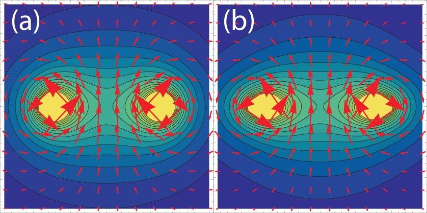
The general solution for a vortex-antivortex (VA) pair is found by taking the sum of two vortex-solutions with opposite winding number, leading to

where $\tilde{x}=x/\tilde{\rho}$, $\tilde{y}=y\tilde{\rho}$ and $\tilde{a}=a/\tilde{\rho}$, with $\tilde{\rho}=(\rho_{xx}/\rho_{yy})^{1/4}$. The parameter $a$ indicates the distance between the cores of a vortex and an antivortex located at $(x=-a,y=0)$ and $(x=a,y=0)$, respectively. Plots of the solution given by Eq. (42) are shown in Fig. 5(a) for the RO case and in 5(b) for the ERD case. The parameters used in this figure are $E_{\rm{B}}/E_{\rm{F}}=0.01$ and $h_{z}/E_{\rm{F}}=0.2$. We chose these parameters to enhance visualization, as the ratio of $\rho_{yy}/\rho_{xx}$ is larger for smaller binding energy.
The emergence of elliptic vortices and the structure of the VA pairs in a 2D Fermi superfluid constitute important signatures for the experimentally relevant ERD case. These signatures could be detected during a time-of-flight expansion of the trapped system, or via Bragg spectroscopy, which is also sensitive to the direction of rotation of the supercurrents [43].
Having discussed the emergence of vortex-antivortex pairs, we investigate next the BKT transition temperature, where vortex-antivortex unbinding occurs.

In this section, we turn to the analysis of the Berezinskii-Kosterlitz-Thouless critical temperature ($T_{\rm{BKT}}$). In order to determine this transition temperature, three equations need to be solved self-consistently: (1) the order parameter equation, determined by the condition $\partial\Omega_{\rm{sp}}/\partial|\Delta|=0$, (2) the number equation $-\partial\Omega_{\rm{sp}}/\partial\mu=n$, and (3) the generalized Kosterlitz-Thouless condition [54] $T_{\rm{BKT}}=\frac{\pi}{2}\rho_{\rm{s}}(T_{\rm{BKT}})$, where $\rho_{\rm{s}}=\sqrt{\rho_{xx}\rho_{yy}}$. The first two equations define the saddle-point (mean-field) ‘transition’ temperature $T_{\rm{MF}}$, at which the system changes from its normal phase with $|\Delta|=0$ to its paired phase with $|\Delta|\neq 0$. However, the transition to a true superfluid phase (quasi-condensate) occurs at $T_{\rm{BKT}}<T_{\rm{MF}}$, which is greatly affected by phase fluctuations. Determining this critical temperature requires the simultaneous solution of all three aforementioned equations.
Here we note that although the equation $T_{\rm{BKT}}=\frac{\pi}{2}\rho_{\rm{s}}(T_{\rm{BKT}})$ was derived originally in the framework of the phase-only XY-model, it is still justified to use it in the present case with spin-orbit coupling. The reason being that the form of the phase-only action with spin-orbit coupling (34), can be re-scaled to the phase-only action without spin-orbit coupling (35). All the effects of spin-orbit coupling are then contained in the ‘effective’ superfluid density $\rho_{\rm{s}}=\sqrt{\rho_{\rm{xx}}\rho_{\rm{yy}}}$. Because the resulting action is still of the same form as the action for the XY-model, the system with and without spin-orbit coupling fall within the same universality class, when the phase transition is continuous. As such, a simple renormalization group analysis leads to the relation $T_{\rm{BKT}}=\frac{\pi}{2}\rho_{\rm{s}}(T_{\rm{BKT}})$, where $\rho_{\rm{s}}$ is the effective superfluid density, defined above.
In Fig. 6, the BKT temperature is shown as a function of the three main system parameters: the spin-orbit coupling strength in (a) and (b), the binding energy in (c) and (d) and the Zeeman field in (e) and (f). Both the equal-Rashba-Dresselhaus (ERD) case and the Rashba-only (RO) case are shown, in the left and right column, respectively. The parameters $v_{\rm{R}},v_{\rm{D}},E_{\rm{B}},h_{z}$ are the main energy scales of the system, and as such their relative magnitude will significantly affect $T_{\rm{BKT}}$, as is discussed in detail below.
We begin by looking at the effect of the spin-orbit coupling strength on the critical temperature. In Fig. (6)(a) and (b), $T_{\rm{BKT}}$ is shown as a function of the spin-orbit coupling strength in the ERD case ($v_{\rm{R}}=v_{\rm{D}}=v$) and the RO case, respectively, for several values of the Zeeman field $h_{z}$. Let us first consider the case without Zeeman field (blue filled circles). In this situation, the spin-orbit strength has no influence on the critical temperature in the ERD case. By contrast, in the RO case, the critical temperature is lowered with increasing spin-orbit coupling. The origin of this difference lies in the nature of the spin-orbit coupling itself. In both the ERD and the RO case, the spin-orbit Hamiltonian can be seen as introducing a gauge field, which leads to orbital motion of the fermions. This makes pairing with opposite momenta harder (orbital frustration), thus suppressing superfluidity.

However, in the ERD case, this gauge field can be removed by a gauge transformation, provided that $h_{z}=0$.
Subsequently, we consider the case of non-zero Zeeman field. In the absence of spin-orbit coupling, it is known that Zeeman fields suppress singlet pairing and thus superfluidity. As shown in Fig.(6)(a) and (b), the introduction of spin-orbit coupling increases the critical temperature compared to the case $v_{\rm{R}}=v_{\rm{D}}=0$. The reason for this is that a triplet pairing component is introduced by the presence of spin-orbit coupling, as was demonstrated in section II.3 where the generalized helicity basis was discussed. This triplet component cannot be suppressed by the Zeeman field.
In the ERD case, $T_{\rm{BKT}}$ rises monotonically and converges to its limiting value without spin-orbit coupling and Zeeman field in the limit $v\rightarrow\infty$. This occurs because in the limit $v\rightarrow\infty$, $h_{z}$ becomes negligible and the effect of ERD spin-orbit coupling can be gauged away. In the RO case, however, the situation is more complex. For $h_{z}=0$, the maximum lies at $v_{\rm{R}}=0$. For low values of $h_{z}$, $T_{\rm{BKT}}$ rises for small values of $v_{\rm{R}}$, reaches a maximum, and then decreases for increasing values of $v_{\rm{R}}$. For high values of $h_{z}$, $T_{\rm{BKT}}$ is a monotonically increasing function of $v_{\rm{R}}$ that never exceeds the limiting value of $T_{\rm{BKT}}$ at $v_{\rm{R}}\rightarrow\infty$.
In Fig. 6(a) and (b) we have encircled two points. These points indicate that the nature of the critical temperature is different there. All other points indicate $T_{\rm{BKT}}$, meaning that the generalized Kosterlitz-Thouless condition $T_{\rm{BKT}}-\pi\rho_{\rm{s}}/2$ is positive for $T>T_{\rm{BKT}}$ and negative for $T<T_{\rm{BKT}}$. However, at these special locations, the situation is different: $T_{\rm{BKT}}-\pi\rho_{\rm{s}}/2$ is still negative for temperatures below this point, but at higher temperatures, the order parameter amplitude $|\Delta|$ is zero, meaning that the mean-field temperature $T_{\rm{MF}}$ has been reached.
In Fig. 6 (c) and (d) the Berezinskii-Kosterlitz-Thouless critical temperature is shown as a function of the binding energy $E_{\rm{B}}$, for different values of the Zeeman field $h_{z}$, for the ERD and the RO cases, respectively. In both figures, the cases with spin-orbit coupling are indicated by symbols, whereas the cases without spin-orbit coupling are indicated by dashed lines. Notice that $T_{\rm{BKT}}$ increases monotonically with increasing binding energy, regardless of the value of the spin-orbit coupling strength. This is as expected, since a larger binding energy leads to more strongly bound fermion pairs, thus strengthening superfluidity. In the asymptotic limit of infinite binding energy, $T_{\rm{BKT}}$ converges to its limiting value: $T_{\rm{BKT}}/T_{\rm{F}}=0.125$, regardless of the strength of the Zeeman field or spin-orbit coupling. This limiting value can be derived from the generalized Kosterlitz-Thouless condition: $T_{\rm{BKT}}=\pi\rho_{\rm{s}}/2$. The superfluid density can at most reach half the total density, where the latter in 2D and in units $\hbar=2m=k_{\rm{F}}=1$ is given by $1/2\pi$. This then leads to $T_{\rm{BKT}}\leq 1/8$. However, when the pairs become bosonic in nature with pair size $\xi_{\rm{pair}}$ much smaller than the interparticle spacing $k_{\rm{F}}^{-1}$, logarithmic corrections due to boson-boson interactions may actually reduce $T_{\rm{BKT}}$, asymptotically [55, 56].
We deliberately chose not to include these logarithmic corrections to the BKT-critical temperature in the present treatment. Including these corrections involves a more complicated calculation, which lies beyond the scope of the present paper. It is important, however, to make sure that we do not reach the regime where logarithmic corrections are relevant. To this end, we have calculated the pair size for the case without spin-orbit coupling (Eq. (19) in [57]) and compared it with the average interparticle distance, given by $k_{F}^{-1}$. In our paper, the latter quantity equals 1 because of our choice of units. In our case, without spin-orbit coupling, for $h_{z}/E_{F}=\{0.01,0.21,0.41\}$ and $E_{B}/E_{F}$ varying between 0.03 and 0.35, the pair size varies between 3.32 and 0.84. Thus, at these values of the binding energy, the regime where $\xi_{\rm{pair}}<<k_{F}^{-1}$ has not been reached, validating our approach.
In the ERD case, we see again that without a Zeeman field, the situations with and without spin-orbit coupling (blue filled circles and blue dashed line, respectively) are exactly equal. When $h_{z}$ becomes non-zero, however, the effect of spin-orbit coupling on the critical temperature is clear, as $T_{\rm{BKT}}$ is significantly increased. The effect is greater where $h_{z}$ is larger. Notice also that while $T_{\rm{BKT}}$ is a smooth curve in the presence of spin-orbit coupling, a jump occurs in the case without spin-orbit coupling, due to a first order phase transition.
The RO case, shown in Fig. 6(d) is qualitatively similar to the ERD case. The main difference is that in the ERD case, at fixed $h_{z}$, spin-orbit coupling increases $T_{\rm{BKT}}$ for all values of the binding energy compared to the case without spin-orbit coupling. By contrast, in the RO case, this increase with respect to zero spin-orbit coupling occurs only at low binding energy, while at large binding energy $T_{\rm{BKT}}$ decreases, because of the aforementioned orbital frustration. The binding energy at which $T_{\rm{BKT}}$ crosses the critical temperature without spin-orbit coupling becomes larger with increasing Zeeman field.
Finally, we study the critical temperature as a function of the Zeeman field $h_{z}$, shown in Fig. 6(e) and (f). The main point of these two figures is the fact that the Clogston limit (i.e. the critical Zeeman field at which the order parameter becomes zero) [58] becomes infinite: the BKT critical temperature only becomes zero in the limit $h_{z}\rightarrow\infty$. This finding is consistent with the zero-temperature behavior, as discussed in section II.5. There, it was shown that the US-1 phase survives all finite values of the Zeeman field. Because our fluctuation theory only describes the 2D system at non-zero temperature it is comforting that the $T\rightarrow 0$ limit is recovered. In the following section, we connect the zero-temperature phase diagram and its quantum phase transition lines to the Berezinskii-Kosterlitz-Thouless critical temperature.

In Fig. 7, we show the finite temperature three-dimensional phase diagram as a function of the two-body binding energy and Zeeman field. This figure connects the zero-temperature phase diagram to the Berezinskii-Kosterlitz-Thouless critical temperature, in the ERD case. The zero-temperature phase diagram is plotted in the $(E_{\rm{B}},h_{z})$-plane. This phase diagram contains three uniform superfluid phases: i-US-0 (red circles), US-2 (blue diamonds) and US-1 (green six-point stars). The BKT critical temperature as a function of $E_{\rm{B}}$ and $h_{z}$ is given by the red translucent surface. This surface only reaches $T=0$ in the limit $h_{z}\rightarrow\infty$ (for all values of $E_{\rm{B}}$), as mentioned in the previous section.
Finally, we have extended the quantum phase transition lines to non-zero temperature. The ‘transition’ between i-US-0 and US-2 is given by the blue surface, and is defined as the finite temperature locus where the quasiparticle nodes of the US-2 phase merge at non-zero momentum, leading to the i-US-0 phase. We find that this ‘transition’ has a small temperature dependence: between $T=0$ and $T_{\rm{BKT}}$ this transition line is displaced by an amount on the order of $0.1h_{z}$. Similarly, the ‘transition’ between US-2 and US-1 is given by the green surface, which has a negligible dependence on temperature.
To the best of our knowledge, no accurate theory exists to calculate the behavior of these lines at non-zero temperature. Here, we obtain these lines based on the quasiparticle description at finite temperatures. This can be regarded as an extrapolation between the zero-temperature results and the Berezinskii-Kosterlitz-Thouless temperature, both of which are known to be qualitatively accurate. Therefore, in the absence of a full theory, it is difficult to claim that these ‘transition’ lines are truly thermodynamic phase boundaries between topologically distinct phases, rather than crossover lines ending at topological phase transition lines at $T=0$. We call them ‘transition’ lines because finite temperature topological invariants can be defined on either side of these lines, provided that a quasiparticle component is still present.