Finite Element Procedures for Enzyme, Chemical Reaction and ’In-Silico’ Genome Scale Networks
Martins, R.C.1, Fachada, N.2
1 Life and Health Sciences Research Institute (ICVS) and
ICVS/3B’s - PT Government Associate Laboratory, Braga/Guimarães, Portugal
Universidade do Minho, Campus of Gualtar, 4710-057 Braga-Portugal
2 ISR – Institute for Systems and Robotics, Instituto Superior Técnico,
Av. Rovisco Pais, 1, 1049-001 Lisboa, Portugal
E-mail: rui.martins@ecsaude.uminho.pt
Abstract
The capacity to predict and control bioprocesses is perhaps one of the most important objectives of biotechnology. Computational simulation is an established methodology for the design and optimization of bioprocesses, where the finite elements method (FEM) is at the state-of-art engineering multi-physics simulation system, with tools such as Finite Element Analysis (FEA) and Computational Fluid Dynamics (CFD).
Although FEA and CFD are currently applied to bioreactor design, most simulations are restricted to the multi-physics capabilities of the existing sofware packages. This manuscript is a contribution for the consolidation of FEM in computational biotechnology, by presenting a comprehensive review of finite element procedures of the most common enzymatic mechanisms found in biotechnological processes, such as, enzyme activation, Michaelis Menten, competitive inhibition, non-competitive inhibition, anti-competitive inhibition, competition by substrate, sequential random mechanism, ping-pong bi-bi and Theorel-Chance.
Most importantly, the manuscript opens the possibility for the use of FEM in conjunction with «in-silico» models of metabolic networks, as well as, chemical networks in order to simulate complex bioprocesses in biotechnology, putting emphasis into flux balance analysis, pheno-metabolomics space exploration in time and space, overcoming the limitations of assuming chemostat conditions in systems biology computations.
Keywords: Finite element analysis, enzyme kinetics, ’in-silico’, genome scale networks
Introduction
Predicting the behavior of bioprocesses is one of the major goals of biotechnology. Computational simulation is today a valuated tool for predicting, monitoring and controlling the status of fermentations, as well as, for optimizing fermentation conditions, minimizing trial and error experimental procedures.
Computational design is recognized as a standard prototyping tool outside the bioengineering area (e.g. automotive and aviation), where it significant reduces costs during design, prototyping and testing phases. All of these, generally involve high experimental load and trained personnel in different areas of research and engineering. The same is also becomming a reality in biotechnology with the advent of systems and synthetic biology.
Traditional experimental methods are limited by the number of recorded parameters for a holistic systems characterization. The conjunction of high-throughput methods (e.g. mass spectroscopy, microarrays, sequencing, spectroscopy and electrochemistry) are today elected for validation of state-of-the-art ’in-silico’ chemical and genome scale models (GSM). Computational simulation provides detailed information in time and space. The Finite Element Method (FEM) is of the ”heart” of many Finite Element Analysis (FEA) and Computational Fluid Dynamics (CFD) software for simulating physical phenomena, such as, heat transfer, mass transfer, radiation, fluid dynamics, structural and elasticity, but it can also be used in biotechnology for simulation of chemical, biochemical reactions, and cellular dynamics [1, 2].
FEM was not initially developed for computational biology and bioprocesses simulation. It has been devoted to industrial prototyping of biotech machinery [3, 4, 5]. It is not yet usual the application of FEM for the simulation of complex biological or chemical systems [6, 7, 8, 9]. In sophisticated developments, FEM has been used to compute microscopic properties, such as: i) the study of membrane elasticity [10]: ii) electrostatic interactions between proteins [11]; iii) mechanical modeling of ion channels [12]; iv) applying FEM in microscopy for physical properties estimation [13]. FEM has also been applied to the study of enzyme kinetics by continuous diffusional biomolecular systems given by the Smoluchwski equation. It has proven to be a good alternative to the traditional spherical criterion model, by allowing to study the complex enzyme geometries [14, 15, 16, 17, 18].
The continuity of FE facilitates the inclusion of other phenomena such as, fluid flow, heat/mass transfer, electromagnetic field, forces and elasticity. The computational cost is less when computing large scale problems described by differential equations, where continuous solutions are common in physical phenomena even at small scales (e.g. force fields, diffusion, heat transfer) [19, 20, 21, 22].
The main steps in FEA involve: i) Pre-processing; ii) Resolving the PDEs or ODEs in the physical-time domain; and iii) post-processing. Pre-processing generally involves: i) ensure that PDEs and ODEs are interactive for multi-physics and chemical, biochemical and microbiological models; ii) ensure that the solution is stable and accurate in the physical-time domain by optimizing the mesh refinement and time steps from computer assisted design software [23, 24, 25] or in more complex geometrics (e.g. biological tissues) by digital scanning and 2D/3D reconstruction methods. This methodology has a number of advantages, such as the treatment of problems on complex irregular shapes, non-uniform meshing to reflect different levels of multi-scale detail, treatment of boundary conditions using continuous solutions and the construction of higher-order approximations to improve accuracy of numerical solutions. Both biological materials, as well as, bioreators display irregular geometries and non-homogeneous physical-chemical properties, which makes difficult to sustain a chemostat hypothesis. FEM not only overcomes such hurdle, but when used in conjunction with inverse problems makes possible to minimizing the error between simulation and experimental datasets obtained in discrete positions of space, to improve model predictions [26, 27, 28]. As biological processes implie multi-physics and multi-scale simulations, it becomes essential to: i) develop the correct relationship between physical-chemical, biochemical and microbiological models; ii) ensure that all used model parameters are correctly determined against experimental data by inverse methods and statistical analysis [29].
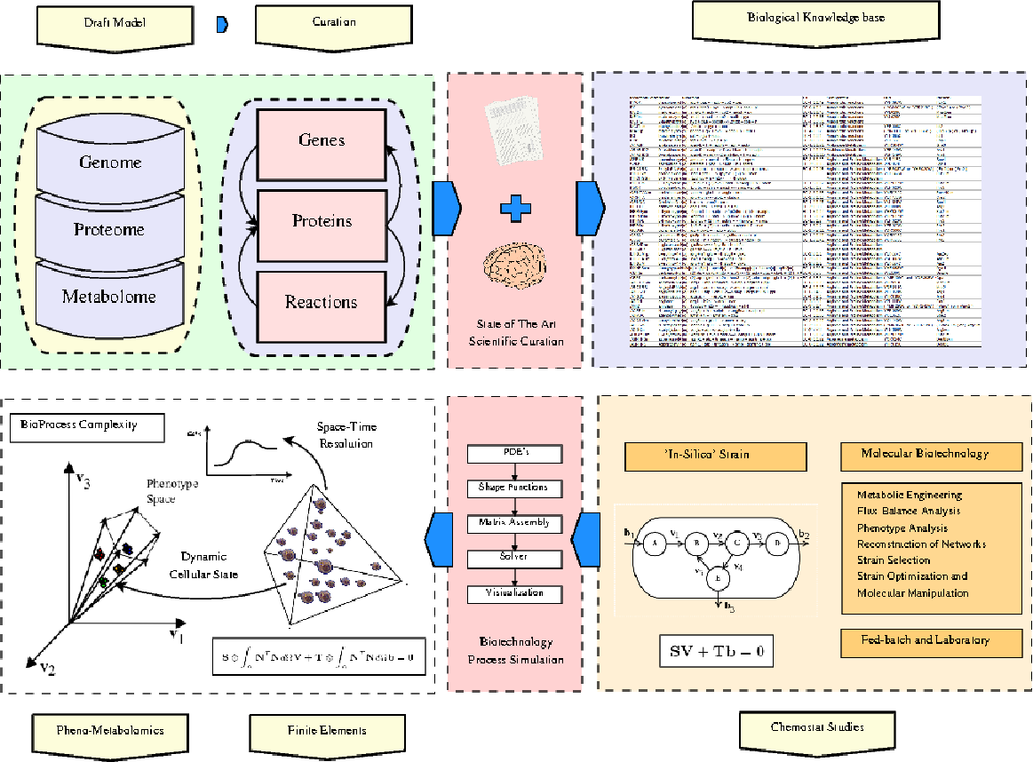
High-throughput molecular biology and analytical chemistry technologies are exponentially increasing chemical and biological ’omics’ information databases (e.g. genomics, metabolomics, transcriptomics, proteomics and protein interactions) (see Figure 1). The available information allowed the emergence of the annotation of gene, protein and metabolic functions, as well as, regulatory mechanisms, so that, network reconstructions of complex biological systems are today feasible. Network models gave rise to the development of ’in-silico’ network organisms, reconstructed from curing the information present in both databases and publications [30, 31], allowing the analysis of network properties and topology, as well as, the comprehensive analysis of cellular functions by systems biology approaches [32].
Connecting all mathematical models on a multi-scale and multi-physics strategy is one of the most important challenges for understanding the complexity of chemical and biological systems [29]. This manuscript is a contribution for the basis of the use of the finite element method procedures for the integration of enzyme kinetics, chemical and genome scale network models (’in-silico’ strains) as a complex systems multi-scale and multi-physics computational modeling research area. This communication is not a comprehensive presentation of the finite elements method, and therefore background on numerical modeling is necessary to make use of the presented equations.
Materials and Methods
The finite elements method
The FEM is considerably different from the most common discretization methodologies, such as Finite Differences (FD), Finite Volumes (FV) and Lattice-Boltzmann (LB) methods. Although elements are geometrically equal, FEM ensures that the solution is continuous inside each element, solved by a weak solutions to a variational optimization of a quadratic problem, being the solution inside a physical given by a piecewise continuity - the shape function.
The following steps resume the FEM methodology: i) Passing from global to local coordinates for the shape function of such element; ii) Variational analysis - determining the solution to the variational problem by weakening the solution inside the finite element; iii) matrix assembly of all equations; and iv) solving [33, 34, 35, 36, 37, 38, 26, 27] and rendering results into graphical mode [37, 28, 39].
The variational method
Changing a Partial Differential Equation (PDE) or an Ordinary Differential Equation (ODE) into the variational form is the main procedure for any FEM discretization. The simplest form of a variational (), states for two continuous functions and :
| (1) |
which means that , a weighting or testing function, can be chosen to force the residuals to be zero inside the finite element interval . The variational problem is posed in the finite element space (). The variational can be solved by the direct substitution of the residuals function () and weighting function () and minimization (Garlekin’s method) or by the minimization of a linear functional (functional method) [34, 40, 41, 42]. The variational method states that there is a solution to the problem of eq. 1 given by:
| (2) |
which satisfies the solution , for any trial function (or shape function). is a bi-linear functional dependent upon the original and trial function and a linear functional dependent only of the trial function. The condition above is only possible to be obtained if the following functional is minimized in the case of 1st order differential equations:
| (3) |
Shape Functions and Elements
Shape function is the continuous approximate solution to the variational problem inside the finite element space. The shape function is only dependent upon the type and shape of the finite element. Elements can be grouped into their different interpolation functions: i) first order - linear elements; ii) second order - quadratic elements, and iii) third order - cubic elements (higher order shape functions are unusual).
The most common FE shape functions are presented in Table 1. These describe a piecewise solution to the variational problem in the physical domain. The FEM is generally used in the natural coordinate system [35]. For example, the subtract concentration inside a linear rectangular element:
| (4) |
where is the enzyme concentration in each of the physical positions inside the element, and , , , at the nodal presents , , and respectively, , , and are the shape coefficients and are dependent on the elements coordinates [34, 40, 41].
The shape function can be presented in the compact matrix format:
| (5) |
where … are the shape coefficients and … the enzyme concentrations at the element nodes to , respectively. The discretization presented in this manuscript can be further extended to the different types of elements using similar mathematical reasoning.
Reaction Models
Reactions in space-time
Diffusion dependent enzyme reactions are well described by the 2nd Fick law:
| (6) |
where is the specimen concentration (), the mass diffusivity (), the force vector and the reaction rate of per unit value (). The simplest reaction term to be added to eq 6 is the first order kinetic:
which can be described by:
| (7) |
where the kinetic rate () is a function of temperature given the modified Arrhenius law. Such states that the decay of is proportional to the probability of finding () molecule inside the finite element space, that is . Consequently, the first order reaction is proportional to its concentration inside the finite element. For the sake of simplicity, lets assume this reaction is occurring inside a linear triangle where is given by:
| (8) |
which is the space distribution of probabilities of finding () inside the finite element space. Therefore, , and map the random movements of molecules inside the finite elements, proportional to speciemens concentration.
Once formulated the variational problem is possible to obtain:
| (9) |
Under these circumstances the variational can be solved by using a linear functional which holds the true solution after the minimization of the bilinear functional :
| (10) |
where the functionals and are given by:
| (11) |
and therefore the functional takes the form of:
| (12) |
Substituting the element functions in the first term of eq. 12, yields:
| (13) |
That once minimised for the node , holds:
| (14) |
The same minimization is necessary to be made in terms of and , to obtain all the elements of the final matrix . After algebraic manipulation, the stiffness matrix () is possible to be described in the matrix format by:
| (15) |
where is the column vector , and the kinetic rate inside the finite element is given by . If one considers as a row vector, than the solution is , since these are symmetric matrices. Similarly, for the second term of eq. 12:
| (16) |
That once minimised in terms of yields:
| (17) |
The same kind of minimization is necessary for and , to obtain the final matrix that will enable the method computation. After algebraic manipulation, the full minimization of the variational is possible to be presented in the matrix format:
| (18) |
Therefore, the chemical reaction can be computed accross the physical domain by:
| (19) |
where presents the probabilities of random movements of the molecule in any direction inside the finite element and the probabilities of effective conformational changes of across the finite element. An important assumption in this discretization, is the fact that kinetic rate is not constant across the physical domain. Such occurs in non-homogeneous biological materials. If one considers constant kinetics, than , where is a constant kinetic rate. For more chemical reaction mechanisms, please consult [2].
Although the 1st order reaction kinetics is the most simplest mechanism, it is still the most widely used to represent both systems chemistry and ’in-silico’ organisms, where single steps are considered uni-molecular, and in the last case, catalyzed by an enzyme, being possible to be used in conjunction with reaction networks and GSM.
Second order kinetics
The simplest form of reaction given by molecular colisions, is the second order reaction kinetic:
where,
| (20) |
and are the concentrations of and specimens inside the finite element. In this case, reaction only occurs once there are effective collisions between and . Therefore, inside any linear finite element the variational form is presented as follows:
| (21) |
where , and vary consistently inside the finite element, taking the form:
| (22) |
which minimizing for node , and , attains:
| (23) |
Which after the variational minimization, the solution yields:
| (24) |
where, , and is the column vector . expresses the frequency of and to react inside the finite element. Afterwards, both equations for and solution must be computed with both equations. Moreover, the term expresses all possible collision probabilities between and specimens inside the finite element. The same is possible to derive for auto-catalyzed reactions (), being possible to show that the solution is held by: .
Results and Discussion
Enzymatic models
Enzyme activation
The enzymatic activation/inactivation is an example of fractional conversion model [43], that describes an equilibrium between two species and , which correspond to inactive and active enzymes, respectively.
In this case, the concentration of and is established by a dynamical equilibrium by:
| (25) | |||
| (26) |
After manipulations, the following finite element formulation inside the linear finite element for inactive and active enzymes, respectively:
Reaction chain
Consider the following reaction chain:
where is the i’th specimen in the reaction chain. By direct comparison with previous formulations it is simple to derive the FEM formulation for each specimen:
The full reaction chain is computed by joining all the specimens equation matrixes.
Michaelis-Menten model
The most widely known enzymatic model is the Michaelis-Menten mechanism:
which can be expressed by a balance to each species:
| (27) |
| (28) |
| (29) |
| (30) |
which inside the finite element can be expressed as:
| (31) |
| (32) |
| (33) |
Inhibition of enzymatic activity
Enzyme inactivation is both a control mechanisms, as well as, a lowering yield factor by an inhibitor (natural or synthetic) which interacts with the enzyme, decreasing the catalytic activity.
Competitive inhibition
Competitive inhibition occurs when an inhibitor () (Figure 2) competes with the substrate for the active center, being represented by:
which can be expressed by a balance to each species:
| (34) |
| (35) |
| (36) |
| (37) |
| (38) |
| (39) |
and after solving the variational problem, the solution can be expressed as:
| (40) |
| (41) |
| (42) |
| (43) |
| (44) |
| (45) |
where and express the frequency of E-S and E-I to react inside the finite element.
Non-competitive inhibition
Non-competitive inhibition occurs when an inhibitor () reversibly establishes a chemical bound with the enzyme which is not the active site, but nevertheless affects its catalytic activity, being possible to be expressed by the mechanism:
which can be expressed by a balance to each species:
| (46) |
| (47) |
| (48) |
| (49) |
| (50) |
| (51) |
| (52) |
which inside the finite element can be expressed as:
| (53) |
| (54) |
| (55) |
| (56) |
| (57) |
| (58) |
| (59) |
where , , , express colliding probabilities of , , and .
Anti-competitive inhibition
When an inhibitor links itself reversibly to enzyme-substrate complex and not to the free enzyme, this is known as anti-competitive inhibition mechanism:
which can be expressed by a balance to each species:
| (60) |
| (61) |
| (62) |
| (63) |
| (64) |
| (65) |
which inside the finite element can be expressed as:
| (66) |
| (67) |
| (68) |
| (69) |
| (70) |
| (71) |
where and express the frequency of and colisions the finite element.
Ping-Pong Bi-Bi mechanism
In Ping-Pong Bi-Bi mechanisms, one of the substrates connects to the enzyme and one of the resulting products releases before the second substrate can connect:
which can be expressed by a balance to each species:
| (72) |
| (73) |
| (74) |
| (75) |
| (76) |
| (77) |
| (78) |
| (79) |
| (80) |
| (81) |
| (82) |
| (83) |
| (84) |
| (85) |
| (86) |
| (87) |
where , , expresses the collision probabilities of , , and , respectively.
| (88) |
| (89) |
| (90) |
| (91) |
where , , expresses the collision probabilities of , , and , respectively.
| (92) |
| (93) |
| (94) |
| (95) |
| (96) |
| (97) |
| (98) |
| (99) |
| (100) |
| (101) |
where , , expresses the collision probabilities of , , and , respectively.
Ping-Pong Bi-Bi with parallel pathway
In some cases, parallel pathways as in Ping-Pong Bi-Bi, such as for DD-carboxypeptidases [44], being an important reaction pattern to be discretized into FEM.
the finite element formulation is presented as:
| (102) |
| (103) |
| (104) |
| (105) |
| (106) |
| (107) |
| (108) |
| (109) |
| (110) |
| (111) |
| (112) |
| (113) |
| (114) |
| (115) |
where , , express the collisions probabilities of , and .
Ternary-complex mechanisms
Ternary-complex mechanism is also common in cellular processes (e.g. DNA polymerase). In this type of enzyme, two substrates need to link to the enzyme to form a ternary complex, either in sequence or random, with the following set of reactions:
which inside the finite element can be expressed as:
| (116) | |||
| (117) |
| (118) |
| (119) |
| (120) |
| (121) |
| (122) |
| (123) |
| (124) |
| (125) |
| (126) |
| (127) |
where , , , express the colision probabilities of , , and , respectively.
Rapid-equilibrium random mechanism
In this mechanism, the enzyme is capable to randomly link to four different substrate (A, B, D) to form the complex EDA or EDB, producing the different molecules P, T and C [45], as follows:
which inside the finite element can be expressed as:
| (128) |
| (129) |
| (130) |
| (131) |
| (132) |
| (133) |
| (134) |
| (135) |
| (136) |
| (137) |
| (138) |
| (139) |
where expresses the frequency of reaction of metabolisms inside the finite element.
Chemical networks
When reactions are put together to describe a chemical system, it can be formalized as a graph, where reactions are links or edges and specimens are nodes (Figure 4). Take for example the following chemical set of reactions:
that can be represented by the graph in Figure 4 (a). In this network, all reactions involve a second order reaction kinetics mechanism, following the FEM discretization presented in section Second order kinetics. If no spacial variation is considered, the differential equation for the presented reaction network is as follows:
| (140) |
where is the reaction rate and the stoichiometry matrix derived from both stoichiometry and reaction graph. For this reaction network, the following system of equations is obtained:
| (141) |
which must be solved by optimization methods. The reaction network can also be represented by an incidence matrix (speciemens relationships) to be used for network topology characterization [46, 47, 48, 49, 50].
Once the chemical system is assumed to be in steady-state, ():
| (142) |
where is the stoichiometric matrix and the specimens flux vector (). The same problem can be derived for the mass-balance of each specimen:
| (143) |
| (144) |
where it can be shown that is equivalent to the 2nd term of eq 141 being therefore an equivalent way of presenting reaction networks. If one considers the concentrations formulation, the reaction network dynamical system across the physical domain is given by:
| (145) |
or for a 1st order reaction kinetics:
| (146) |
or by joining different mechamisms:
| (147) |
Where and handle all the stoichiometric relationships between specimens.
In chemical systems, network reconstruction is harder to cure when compared with biochemical data. Information is still scattered throughout publications and less efforts have been put into reconstructing chemical systems, such as in atmospheric science and foods. For example, Figure 4 (b) presents part of known ascorbic acid (AA) degradation pathways [51, 52]. The full understanding of the AA degradation has major impact on both nutrition and quality of foods, but it still lacks the major mechanistic steps and thermodynamics. The same is valid for many important aging and degradation mechanism which involve oxidation [53]. The reconstruction of this network implies the existence of high-throughput analytical chemistry dedicated facilities and bioinformatics, so that complex systems approaches can be applied to this research area [2].
As there is incomplete information, network simulation has to rely on flux analysis and measurements of flux rates instead of concentrations, kinetic rates, catalysis and Arrhenius activation energies. Considering that fluxes inside a triangular finite element is given by the shape function:
| (148) |
where, , and are the specimen flux at nodal positions , and ; and the variational problem is resumed to:
| (149) |
that once minimised for the node , helds:
| (150) |
and performing for all nodal positions and chemical specimens, is possible to conclude the final matrix format:
| (151) |
Where all stoichiometric relationships inside the FE space are respected, because:
| (152) |
| (153) |
where is a zero squared matrix, and expands into a colum vector (21,1):
| (154) |
Where all fluxes can be computed for any region of space.
The same problem can be discretized using the stoichiometric matrix in eq 141, where in complex chemical systems can be assembled from a knowledge base database table (Figure 4), where reactions, specimens, stoichiometric factors, presence of catalysts, flux code and activation energies are cataloged, to obtain a linear system , where in this example, , and , and , respectively.
It can shown that inside any finite element, the set of equations became:
| (155) |
where for a triangular finite element,
| (156) |
Being the solution for any given chemical network solve accross the physical domain as:
| (157) |
In many cases, reaction mechanisms are not fully understood and incomplete analytical chemistry may not allow to derive all time-course dependencies in chemical systems. For engineering purposes, empirical pseudo-reaction steps can be assumed in incomplete reaction networks, such as for the ascorbic acid oxidation presented in Figure 4 (b). The same formulation is possible to be presented to the pseudo-mechanistic network while there is not total knowledge about all reaction mechanisms (e.g. computational shelf-life dating [29]).
Effect of temperature and catalysts
Pure chemical systems can be considered ’auto-regulated’ by thermodynamics, that is, mechanical properties, kinetic and equilibrium constants, activation energies and presence of catalysts. Chemical reactions dependence on temperature are generally modeled by the Arrhenius relationship:
| (158) |
where and are the kinetic rates at temperature and (K), respectively; the Arrhenius activation energy (). The effect of catalysts can be reflected in the decrease of , allowing the same reactions to occur at faster rates at lower temperatures.
In order to reflect the effect of both temperature and catalysts, a weight matrix is possible to be deduced, as the fraction of the kinetic rate of a reaction step by it’s reference kinetic rate:
| (159) |
demonstrating that under steady state the integration is given by , with the corresponding finite element formulation:
| (160) |
where . Furthermore, when the reaction step is deleted (e.g. deletion of a catalyst), reactions are slower than the reference temperature, and otherwise, enabling to study chemical systems under different environmental conditions.
’In-Silico’ genome scale networks
Modeling cellular growth had a significant impact on biotechnology in the pre-genomic era. Models with macroscopic assumptions, also know as ’predictive microbiology’ (e.g. [54, 55, 56]) are still used due to their simplicity of assumptions and availability of information on kinetic data. FEM formulations were already derived for many of these models and can be found in [2].
The implementation of high-throughput methodologies in molecular biology (e.g. genome sequencing, electrophoresis, protein sequencing, mass spectroscopy, NMR), automated cellular manipulation (e.g. gene knock-out) [57] and the emergence of bioinformatics, provide that gene functions, protein specificity and partial metabolic networks are available in several species (e.g. ecoli, yeast and human) in databases such as, BioCyc [58], SGD [59], KEGG [60] , Reactome [61], UniProt [62]. With the increasing datasets, the development and update of holistic ’in-silico’ genome-scale network draft models (GSM) has became possible to be automated [63, 64] for further validation by human experts to provide ’in-silico’ model organisms (Figure ).
There are three main types of ’in-silico’ GSM models: i) interaction network models; ii) steady-state stoichiometric networks; and iii) dynamical models (e.g. ECELL [65]). The latest are yet less used because of the lack of reliable ’in-vivo’ kinetic data, and therefore, interaction and steady state models are dominant in bioinformatics and systems biology analysis. Genome scale models can be further classified into non-compartmentalized and compartmentalized models (e.g. IND750 [30], IMM940 [66]). The second class, accounts for metabolic networks contained in the different organelles and transport reactions between organelles, cytoplasm and extracellular space. Substantially complete models are available for ecoli (1260 genes, 2077 reactions, 690 of transport, 1039 metabolites), s. cerevisiae (e.g.IND750, 750 genes, 648 metabolites, 1149 reactions, 297 of transport) and many other organisms in the BIGG database [67].
0.0.1 Flux-Balance Analysis
Considering the example network inside an organism presented in Figure , at any given position of space inside a finite element domain, the concentration of metabolites of the ’in-silico’ organism can be given by:
| (161) |
where is the stoichiometric matrix, the metabolite flux (mol/s), the growth rate (). In most conditions, as kinetic constants are not available ’in-vivo’, these models use the flux instead of the traditional kinetic constants. However, , where at a given time or space position. Moreover, network studies assume pseudo steady-state conditions at a given time, that is, fluxes considered stable under short time periods, when compared to population growth and concentration of metabolites. The problem resumes to:
| (162) |
which for the network model is:
| (163) |
Taking into consideration a consistent spacial gradient of the flux at any position, the solution is given by the minimization of the variational:
| (164) |
and therefore, for a given metabolite , the spacial solution is given by:
| (165) |
where all network reactions are taken into account inside the finite element space by using the Kronecker product with the stoichiometric matrix. Note that is a column vector that spawns all vertices’s fluxes, such as, for a triangular finite element .
This simple formulation allows to perform FBA in conjunction with multi-physics FEM or CFD simulation in any biotechnological processes. In this sense, a state-of-the-art genome scale model analysis can be performed now with spatio-temporal resolution and in the complex scenario that modelers want to set-up for simulation, by integrating FEM solutions with systems biology to provide a genome scale diagnostic at any point of the FE mesh, such as the functionalities presented in [68].
State-of-the-art GSM were designed to assist molecular biology research, assuming chemostat conditions, and not for bioprocess or complex systems simulations. Today’s GSM cannot cope with: i) complex enzymatic mechanics; ii) kinetics and temperature effect; iii) dynamical states; iv) concentrations of metabolites; v) temporal and spacial resolution; vi) multi-physics phenomena are not taken into account (e.g. heat transfer, diffusion, fluid flow) and v) pathways are always assumed to be optimal, where control or thermodynamic restrictions are implemented by flux constrains.
GSM provide today many applications in biotechnology, such as: i) flux balance analysis (FBA) for strain optimization; ii) network topological analysis, reliability, viability, structural homology; iii) derivation of phenotype spaces for the exploration of biodiversity and biotechnological potential (Figure 5). As these models do not hold a particular solution, both null space, convex analysis and optimization methods are applied to explore the solution space in chemostat conditions (e.g. MOMA, ROOM, genetic algorithms) [68]. Furthermore, as solutions may converge into different regions of the phenotype, being necessary to develop new space basis, such as, the development of elementary flux analysis [69, 70, 71] and extreme pathways [72, 73, 74].
The integration of GSM with FEM allows to overcome many of the previously mentioned barriers, allowing to perform genome-scale analysis of cells in the context of spatio-temporal conditions in a multi-physics environment [2]. Figure 5 exemplifies the integration. GSM are a set of incidence matrices, computationally derived from databases and cured with publications and expert analysis, relating genes to enzymes, enzymes and reactions, and, reactions to metabolites which given the stoichiometric relationships can be expressed as internal and boundary fluxes of metabolites.
When deriving the GSM inside the finite element, the ’in-silico’ organism becomes dependent on the external conditions of nutrients, temperature, fluid flow, as well as, being affected by neighboring cells in any part of the physical and time domains. FEM considers that GSM is continuously discretized across the physical domain; at any point of the physical domain all metabolite fluxes and phenotype space is possible to be characterized, such as, for example the coordinates inside the convex hull given by the extreme pathways (see Figure 5, with limitless applications in biotechnology.
Compartimented models
In fully compartmentalized GSM models, each cellular organelle has an internal metabolic network, enzymes and associated genes. Common metabolites among compartments are linked by transport fluxes [30, 66]. In this reasoning, steady state equations resume to:
| (166) |
where is the transport incidence matrix and the boundary fluxes. After concatenation of all organelles metabolism and transport equations, cellular state inside a FE space is given by:
| (167) |
Being by this equation characterizes ’in-silico’ compartimentalized organisms at any region of the finite element space .
Pheno-metabolomics
Pheno-metabolomics plays a major role in post-genomic biotechnology. The exploration of the phenotype and metabolic capacities of organisms with the aid of both high-throughput methods in conjunction with genome scale models and complex systems simulation tools lies at the heart of pheno-metabolomics bioinformatics. Our research center has an important biodiversity yeast biobank, with especial emphasis on Saccharomyces cerevisiae isolates, and has been working in the characterization of S. cerevisiae over the last decade of yeast from different ecological contexts and geographical origins for their phenotype potential [75, 76].
The pheno-metabolome of species is highly diversified, but most particular solutions of GSM have been restricted to the validation of simple, controlled experimental conditions [30] which do not reflect the complexity of real-world bioprocess and natural conditions where yeasts evolved, lacking the design of new tools to both detect and derive new mechanisms as well as to cope with the dynamical complexity of cells. The use of GSM has been restricted to the assessment of the phenotype space derived from the stoichiometric matrix, being necessary to develop new approaches to fully explore the biodiversity of biobanks, evolution and adaptation mechanisms, as well as, the discovery of unknown mechanism by integration of GSM with both high-throughput signal processing, statistical computing, process analytical technology and computational simulation in order to be possible do derive the most correct definition of the phenotype space.
One of the first approaches to define the phenotype of species was proposed as a non-negative linear combination of all relationships present in the stoichiometric matrix, holding all non-negative possible solutions of , when all fluxes [77]. Such geometry is defined by the non-negative combination of a new vector basis, forming a convex hull defined by extreme rays (or pathways):
| (168) |
where is the convex space (see Figure 1) delimited by the extreme pathways and the coordinates projected into each . Note that is not an orthogonal basis, and only delimits the solution space of , being the vectors presented in Figure 1 in the natural basis of , which is not a practical visualization method once most GSM are hyper-dimensional. can be obtained by the methodology presented in [77], and hold important properties for the interpretation of the phenotype space: i) primary metabolism linked to boundary fluxes; ii) futile cycles with link to boundary fluxes; and iii) internal cycles.
Inside a FE, the convex hull coordinates of any point are possible to be described by the element shape function (or in any other basis):
| (169) |
allowing to apply finite element analysis (FEA) techniques do diagnose space differentiation in phenotype and metabolic state on the extreme pathways vector basis .
Spacio-temporal analysis
Spacio-temporal analysis is perhaps one of the major advantages of joining FEM and GSM, becaming possible to analyze how the metabolic state evolves throughout space-time, as well as, to access how different phenotypes respond to different environment conditions. Previous sections already presented how to include fluxes () and pheno-metabolome coordinates () on a finite element domain. Such allows to analyze emergent patterns in cell communities and perform systems biology analysis [68] at each region of space the cause of phenotype differences. Such tool will become more and more important, as cellular morphology may became manageable inside bioreactors [78, 79].
For instance, the use of the FEM allows to derive space vector gradients of both fluxes and phenotypes:
| (170) |
where is the gradient property to be analysed across the physical domain.
FEA may be used to further explore the phenotype dynamics, where for example the space derivate allows to determine geometrical changes in phenotypes across the FE domain (e.g. change rate () and acceleration ()):
| (171) | |||
| (172) |
Allowing to explore dynamically the molecular biology of different phenotypes, such as, the determination of the most important pathways and cellular functions at different stages, understand enzyme efficiency and metabolic rates, regulation mechanisms and transcription rates in different contexts of cellular growth, as well as, understanding accelerations in phenotype changes or metabolic states as adaptations to changes in the environment. Figure 5 resumes the use of the phenotype coordinates with FEM.
As the solution of GSM equations is in many cases stochastic [68], it is also important to be able to visualize the statistics of predictions in the FE domain. For example, is possible to derive both expected phenotype and corresponding variance on a surface:
| (173) |
| (174) |
where is the finite element surface area () [2].
As this new approach may provide many possible solutions in the phenotype space, and therefore inverse FEM methods coupled with real-time and high-throughput experimental methods in molecular biology will be necessary to fine tune the numerical results of FEA analysis. Table 2 presents analogies between FEM-GSM and biological implications. Moreover, as dynamical results can be complex in terms of interpretation, pattern recognition recurring to compressed space coordinates may be more appropriate than direct visualization of fluxes and phenotype coordinates.
The integration of FEM with reaction networks and genome scale networks will play an important role in the simulation and diagnostic of complex biological systems in the near future. Systems biology and systems chemistry lacked the possibility of integrating systems knowledge with multi-physics and multi-scale physics with 4D discretization that may enable in the future the computational assessment of phenotype tests, such as diagnostic the metabolic states under different growth media, emergence effects of gene deletion and stress factors, as well as bioengineering issues such as, reactor temperature, must composition and bioreactor design. This kind of tools will also open new possibilities in deriving and exploring the phenotype space for effective exploration of biobanks, providing critical informations for the decision of strain selection or improvement for a given biotechnological process. This manuscript is an introduction to the endless possibilities that are open for both study of complexity by FEM and network models and use of this methodology for the exploration of phenotypes, diagnosis, modeling, simulation and control of complex bioprocesses.
Acknowledgments
This work was finantially supported by the Fundação para a Ciência e Tecnologia, projects OpenMicrobio (PTDC/BIO/69310/2006) - A framework for the simulation of cellular communities during bioprocess engineering, Phenomet (PTDC/AGR-ALI/103392/2008 FEDER/COMPETE). The funders had no role in study design, data collection and analysis, decision to publish, or preparation of the manuscript.
References
- 1. Martins R (2006) Finite volumes and finite element procedures for foods quality and safety simulations. Journal of Food Engineering 73: 327-338.
- 2. Martins R, Lopes V, Vicente A, Teixeira J (2009) Numerical solutions: Finite element and finite volume methods. In: Erdogdu F, editor, Optimization in Food Engineering. London, England: CRC Press, pp. 377-418.
- 3. Davidson K, Sushil S, Eggleton C, Marten M (2003) Using computational fluid dynamics software to estimate circulation time distributions in bioreactors. Biotechnology Progress 19(5): 1480-1486.
- 4. Ghadge R, Patwardhan A, Joshi J (2006) Transport in a grooved perfusion flat-bed bioreactor for cell therapy applications. Biotechnology Progress 22(3): 660-672.
- 5. O-Charoen S, Srivannavit O, Gulari E (2007) Simulation and visualization of flow pattern in microarrays for liquid phase oligonucleotide and peptide synthesis. Biotechnology Progress 23(3): 755-761.
- 6. Geller S, Krafczyk M, Tölke J, Turek S, Hron J (2006) Benchmark computations based on lattice-boltzmann, finite element and finite volume methods for laminar flows. Computers & Fluids 35: 888-897.
- 7. Kashid M, Agar D, Turek S (2007) Cfd modelling of mass transfer with and without chemical reaction in the liquid-liquid slug flow microreactor. Chemical Engineering Science 62: 5102-5109.
- 8. Munthe O, Langtangen H (2000) Finite elemetns and object-oriented implementation techniques in computational fluid dynamics. Computer Methods in Applied Mechanics and Engineering 190: 865-888.
- 9. Shepel S, Smith B (2006) New finite-element/finite-volume level set formulation for modelling two-phase incompressible flows. Journal of Computational Physics 218: 479-494.
- 10. Hansen J, Skalak R, Chien S, Hoger A (1997) Influence of network topology on the elasticity of the red blood cell membrane skeleton. Biophysics Journal 72: 2369-2381.
- 11. Zhou H (1993) Boundary element solution of macromolecular electrostatics: interaction energy between two proteins. Biophysics Journal 65: 955-963.
- 12. Tang Y, Cao G, Chen X, Yoo J, Yethiraj A (1999) A finite element framework for studying the mechanical response of macromolecules: application to the gating of the mechanosensitive channel mscl. Biophysics Journal 91(4): 1248-1263.
- 13. Charras G, Horton M (2002) Determination of cellular strains by combined atomic force microscopy and finite element modeling. Biophysics Journal 83: 858-879.
- 14. Elcock A, Putter M, Mathews D, Knighton J DR McCammon (1999) Electrostatic channeling in the bi-functional enzyme dihydrofolate redutase-thymidylase synthase. Journal of Molecular Biology 262: 370-374.
- 15. Elcock A, Sept D, McCammon J (2001) Computer simulation of protein-protein interactions. Journal of Physical Chemistry B 105: 1504-1518.
- 16. Gadzouline R, Wade R (1998) Brownian dynamics simulation of protein-protein diffusional encounter. Methods 14: 329-341.
- 17. Tara S, Elcock A, Kirchhoff P, Briggs J, Radic Z, et al. (1998) Rapid binding of a cationic active site inhibitor to wild type and mutant mouse actetylcholinestrease: Brownian dynamics simulation including diffusion in the active site gorge. Biopolimers 46: 465-479.
- 18. Radic Z, Kirchhoff P, Quinn D, McCammon J, Taylor P (1997) Electrostatic influence on the kinetics of ligand bindings to acetylcholinesterase - distintions between active center ligands and fasciculin. Journal of Biological Chemistry 272(37): 23265-23277.
- 19. Drury J, Dembo M (1999) Hydrodynamics of micropipette aspiration. Biophysics Journal 76: 110–128.
- 20. Sachs F (1999) Practical limits on the maximal speed of solution exchange for patch clamp experiments. Biophysics Journal 77: 682-690.
- 21. Song Y, Zhang Y, Bajaj C, Baker N (2004) Continuum diffusion reaction rate calculations of wild-type and mutant mouse acetylcholinesterase: Adaptive finite element analysis. Biophysics Journal 87: 1558-1566.
- 22. Watanabe H, Sugiura S, Kafuku H, Hisada T (2006) Multiphysics simulation of left ventricular filling dynamics using fluid-structure interaction finite element method. Biophysics Journal 87: 2074-2085.
- 23. Fluent (2004). Fluent, the right answer in cfd. URL http://www.fluent.com/.
- 24. Ansys (2004). Ansys multyphysicsTM 8.0. URL http://www.ansys.com/.
- 25. CFX (2004). Computational fluid dynamics software and services. URL http://www-waterloo.ansys.com/cfx/.
- 26. Chen Z (2005) Finite element methods and their applications. New York: Springer-Verlag. 414p.
- 27. Thomeé V (2006) Garlekin finite element methods for parabolic problems. Heidelberg: Springer-Verlag, 2nd edition. 382p.
- 28. Nakasone Y, Yoshimoto S, Stolarski T (2006) Engineering analysis with ANSYS. Amsterdam: Elsevier. 473p.
- 29. Martins R, Lopes V, Vicente A, Teixeira J (2008) Computational shelf-life dating: Complex systems approaches to food quality and safety. Food Bioprocess Technology 1: 207-222.
- 30. Duarte N, Herrgard M, Palsson B (2004) Reconstruction and validation of Saccharomyces cerevisiae ind750, a fully compartimentalized genome-scale metabolic model. Genome Research 14: 1298-1309.
- 31. Herrgard M, Fong S, Palsson B (2006) Identification of genome-scale metabolic network models using experimentally measured flux profiles. PLoS ComputBiol 2(7): e72. DOI: 10.1371/journal.pcbi.0020072.
- 32. Nielsen J, Jewett M (2008) Impact of systems biology on metabolic engineering of sacharomyces cerevisiae. FEMS Yeast Research 8: 122-131.
- 33. Strang G, Fix G (1997) An Analysis of the Finite Element Method. New Jersey: Prentice Hall Inc.
- 34. Segerlind L (1984) Applied Finite Element Analysis. New York: Macmillan Press, LTD, 2 edition.
- 35. Henwood D, Bonet J (1996) Finite Elements, A Gentle Introduction. London, England: Macmillan Press, LTD.
- 36. Braess D (1997) Finite Elements. Theory, Fast Solvers, and Applications in Solid Mechanics. Cambridge: Cambridge University Press.
- 37. Moaveni S (1999) Finite element analysis - theory and applications with ANSYS. Amsterdam: Elsevier. 272p.
- 38. Hutton DV (2004) Fundamentals of finite element analysis. London, England: McGraw-Hill Book Co. 505p.
- 39. VTK (2007). The visualisation toolkit. URL http://www.vtk.org/.
- 40. Rozanov Y (1998) Random Fields and Stochastic Partial Differential Equations. London, England: Kluwer Academic Publishers. Mathematics and Its applications.
- 41. Ghanem R (1991) Stochastic Finite Elements: a Spectral Approach. New York: Springer-Verlag.
- 42. Nicolai BM, Scheerlink N, Verboen P, Baerdemaker JP (2000) Stochastic perturberation analysis of thermal food process with random fields parameters. Transactions of the ASAE 43(1): 131-138.
- 43. Villota R, Hawkes J (1992) Reaction kinetics in food systems. In: Valentas K, Rotstein E, Singh R, editors, Handbook of Food Engineering. New York: Marcel Dekker, Inc, pp. 39–144.
- 44. Frére J (1973) Enzymatic mechanims involving concomitant transfer and hydrolysis reactions. Biochemistry Journal 135: 469-481.
- 45. Alberty B (2009) Determination of rapid equilibrium kinetic parameters of ordered and random enzyme catalyzed reaction a + b = p + o. Journal of Chemical Physics 113: 10043–10048.
- 46. Albert R, Barabasi A (2002) Statistical mechanics of networks. Reviews of Modern Physics 74: 47–97.
- 47. Dorogovtsev S, Mendes J (2003) Evolution of networks: from biological nets to the internet and www. Oxford: Oxford University Press.
- 48. Barabasi A, Bonabeau E (2003) Scale-free networks. Scientific American 288: 50–59.
- 49. Barabasi A (2007) The architecture of complexity. IEEE Control Systems Magazine 27(4): 33–42.
- 50. Barabasi A (2009) Scale-free networks - a decade and beyond. Science 325: 412–413.
- 51. Bauernfeind J, Pinkert D (1970) Food processing with added ascorbic acid. Adv in Food Research 18: 219–315.
- 52. Tannenbaum S (1985) Vitamins and minerals. New York: Marcel Dekker, Inc, pp. 477-544.
- 53. Martins ea (2008) Oxidation management of white wines using cyclic voltammetry and multivariate process monitoring. J Agric Food Chem 56(24): 12092 – 12098.
- 54. McKellar R (1997) A heterogeneous population model for the analysis of bacterial growth kinetics. International Journal of Food Microbiology 36: 179-186.
- 55. Baranyi J, Pin C (1999) Estimating bacterial growth parameters by means of detection times. Applied and Environmental Microbiology 65: 732–736.
- 56. McKellar RC, Knight KP (2000) Combined discrete-continuous model describing the lag phase of Listeria monocytogenes. International Journal of Food Microbiology 54: 171–180.
- 57. King Rea (2011) The automation of science. Science 324: 85–89.
- 58. BioCyc (2012). Biocyc - a collection of 1690 pathway/genome databases. URL: http://biocyc.org/.
- 59. SGD (2012). Yeast genome database. URL: http://www.yeastgenome.org/.
- 60. KEGG (2012). Kyoto encyclopedia of genes and genomes. URL: http://www.genome.jp/kegg/.
- 61. Reactome (2012). Curated knowledgebase of biological pathways in humans. URL: http://www.reactome.org/.
- 62. UniProt (2012). Comprehensive, high-quality and freely accessible resource of protein sequence and functional information. URL: http://www.uniprot.org/.
- 63. DeJongh M, Formsma K, Boillot P, Gould J, Rycenga M, et al. (2007) Toward the automated generation of genome-scale metabolic networks in the seed. BMC Bioinformatics 8: 139.
- 64. DeJongh M, Formsma K, Boillot P, Gould J, Rycenga M, et al. (2010) High-throughput generation, optimization and analysis of genome-scale metabolic models. Nature Biotechnology 28: 977–982.
- 65. Takashi K, Ishikawa N, Sadamoto Y, Sasamoto H, Ohta S, et al. (2003) E-cell 2: Multi-platform e-cell simulation system. Bioinformatics 19: 1727–1729.
- 66. Mo ML, Palsson BO, Herrgåard MJ (2003) Connecting extracellular metabolomic measurements to intracellular flux states in yeast. BMC Systems Biology 3: 37.
- 67. Schellenberger J, Park JO, Conrad TC, Palsson B (2010) Bigg: a biochemical genetic and genomic knowledgebase of large scale metabolic reconstructions. BMC Bioinformatics 11: 213.
- 68. Schellenberger J, Que R, M FR, Thiele I, D OJ, et al. (2011) Quantitative prediction of cellular metabolism with constraint-based models: the cobra toolbox v2.0. Nature Protocols 6(9): 1290–1307.
- 69. Gayen K, Venkatesh KV (2006) Analysis of optimal phenotypic space using elementary modes as applied to corynebacterium glutamicum. BMC Bioinformatics 7: 445.
- 70. Kim JI, Varner JD, Ramkrishna D (2006) A hybrid model of anaerobic e. coli gjt001: combination of elementary flux modes and cybernetic variables. Biotechnol Progress 24(5): 993-1006.
- 71. Beurton-Aimar M, Beauvoit B, Monier A, Vallée F, Dieuaide-Noubhani M, et al. (2003) Comparison between elementary flux modes analysis and 13c-metabolic fluxes measured in bacterial and plant cells. BMC Systems Biology 5: 95.
- 72. Papin JA, Price ND, Palsson BO (2002) Extreme pathway lengths and reaction participation in genome-scale metabolic networks. Genome Research 12(12): 1889-1900.
- 73. Price ND, Reed Rl, Famili I, Palsson BO (2003) Analysis of metabolic capabilities using singular value decomposition of extreme pathway matrices. Biophysics Journal 84: 794-804.
- 74. Famili I, Mahadevan R, Palsson BO (2005) k-cone analysis: Determining all candidate values for kinetic parameters on a network scale. Biophysics Journal 83(3): 1616–1625.
- 75. Schuller D, Casal M (2007) The genetic structure of fermentative vineyard-associated Saccharomyces cerevisiae populations revealed by microsatellite analysis. Antonie van Leeuwenhoek 91(2): 137-150.
- 76. Franco-Duarte R, Umek L, Zupan B, Schuller D (2009) Computational approaches for the genetic and phenotypic characterization of a saccharomyces cerevisiae wine yeast collection. Yeast 26(12): 675-692.
- 77. Schilling CH, Letscher D, Palsson BO (2000) Theory for the systemic definition of metabolic pathways and their use in interpreting metabolic function from a pathway-oriented perspective. Journal of Theoretical Biology 203(3): 229–248.
- 78. Castro C, Silva J, Lopes V, Martins R (2009) Yeast metabolic state identification by fiber optics spectroscopy. BioSignals 2009 1: 1-12.
- 79. Silva R, Silva J, Teixeira J, Martins R (2009) In-situ, real-time bioreactor monitoring by fiber optic sensors. BioSignals 2009 1: 12-24.



| Element | Interpolation Polynomial | Shape Function |
|---|---|---|
| Linear Beam | ||
| Linear Triangle | ||
| Linear Quadrilateral | ||
| Linear Tetrahedron | ||
| Linear Cube | ||
| Quadratic Beam | ||
| Quadratic Triangle | ||
| Quadratic Quadrilateral | ||
| Quadratic Tetrahedron | ||
| Quadratic cube | ||
| Finite Element | Biology | |
|---|---|---|
| Phenotype spacial distribution | ||
| Phenotype statistical distribution | ||
| Rate of cellular differentiation | ||
| Rate of cellular adaptation | ||
| Phenotype spacial differentiation vector |