Minority population in the one-dimensional Schelling model of segregation Thanks: Authors are listed alphabetically. Barmpalias was supported by the 1000 Talents Program for Young Scholars from the Chinese Government, and the Chinese Academy of Sciences (CAS) President’s International Fellowship Initiative No. 2010Y2GB03. Additional support was received by the CAS and the Institute of Software of the CAS. Partial support was also received from a Marsden grant of New Zealand and the China Basic Research Program (973) grant No. 2014CB340302. Lewis-Pye was supported by a Royal Society University Research Fellowship. We would like to thank Pan Peng and Zhang Wei from the Institute of Software of the CAS, for helpful discussions.
Abstract
The Schelling model of segregation looks to explain the way in which a population of agents or particles of two types may come to organise itself into large homogeneous clusters, and can be seen as a variant of the Ising model in which the system is subjected to rapid cooling. While the model has been very extensively studied, the unperturbed (noiseless) version has largely resisted rigorous analysis, with most results in the literature pertaining to versions of the model in which noise is introduced into the dynamics so as to make it amenable to standard techniques from statistical mechanics or stochastic evolutionary game theory.
We rigorously analyse the one-dimensional version of the model in which one of the two types is in the minority, and establish various forms of threshold behaviour. Our results are in sharp contrast with the case when the distribution of the two types is uniform (i.e. each agent has equal chance of being of each type in the initial configuration), which was studied in [BIKK12, BELP14].
George Barmpalias
State Key Lab of Computer Science,
Institute of Software, Chinese Academy of Sciences, Beijing, China.
School of Mathematics, Statistics and Operations Research,
Victoria University of Wellington, New Zealand.
E-mail: barmpalias@gmail.com.
Web: http://barmpalias.net
Richard Elwes
School of Mathematics,
University of Leeds, LS2 9JT Leeds, United Kingdom.
E-mail: r.h.elwes@leeds.ac.uk.
Web: http://richardelwes.co.uk
Andy Lewis-Pye
Department of Mathematics,
Columbia House, London School of Economics,
Houghton Street, London, WC2A 2AE, United Kingdom.
E-mail: A.Lewis7@lse.ac.uk.
Web: http://aemlewis.co.uk
1 Introduction
The economist Thomas Schelling introduced his model of segregation in [Sch69] (developed later in [Sch71a, Sch71b]), with the explicit intention of explaining the phenomenon of racial segregation in large cities. Perhaps the earliest agent-based model studied by economists, since then it has become an archetype of agent-based modelling, prominently featuring in libraries of modelling software tools such as NetLogo [Wil99] and often being the subject of experimental analysis and simulations in the modeling and AI communities [CMGP13, CM11, Fos06, GB02, Sch07, YÖ09, HCSB11, dSGL07, EA96]. Many versions of the model have been analysed theoretically, from a number of different viewpoints and disciplines: statistical mechanics [DCM08, CFL09] and [Ber12, Section 3.1], evolutionary game theory [You98, Zha04a, Zha04b, Zha11] the social sciences [CF08, Cla91, SSD00], and more recently computer science and AI [CACP07, BMR14, BIKK12, BELP14]. It was observed in [BIKK12], however, that despite the vast amount of work that has been done on the Schelling model in the last 40 years, rigorous mathematical analyses in the previous literature generally concern altered versions of the model, in which noise is introduced in the dynamics, i.e. where one allows that agents may make non-rational decisions that are detrimental to their welfare with small probability. The introduction of such ‘perturbations’ may be justifiable from a ‘bounded rationality’ standpoint.
The model (which will be formally defined shortly) concerns a population of agents arranged geographically, each being of one of two types. Each agent has a certain neighbourhood around them that they are concerned with, and also an intolerance parameter which we shall assume here to be the same for all agents. An agent’s behaviour is dictated by the proportion of the agents in their neighbourhood which are of its own type. So long as this proportion is the agent may be considered ‘happy’ and will not move. Starting with a random configuration, one then considers a discrete time dynamical process. At each stage unhappy agents may be given the opportunity to move, swapping positions with another agent, so as to increase the proportion of their own type within their neighbourhood. Now one might justify a perturbed version of these dynamics, in which agents will occasionally move in such a way as to decrease their utility (i.e. the proportion of their own type within their neighbourhood) by arguing, for example, that it is reasonable to suppose that only incomplete information about the make-up of each neighbourhood is available to the agents. It is a fact, however, that
- (a)
the methods used for the analysis of the perturbed models do not apply to the unperturbed model;
- (b)
the segregation that occurs in the perturbed models is often very different than in the unperturbed model.
In the unperturbed models the underlying Markov chain does not have the regularities that are found in the perturbed case (e.g. the Markov process is irreversible). The presence of a large variety of absorbing states means that entirely different and more combinatorial methods are now required. Beyond the basic aim of a rigorous analysis for these unperturbed models, which have been so extensively studied via simulations, further motivation is provided by the fact that the Schelling model is part of a large family of models, arising in a broad variety of contexts—spin glass models, Hopfield nets, cascading phenomena as studied by those in the networks community—all of which look to understand the discrete time dynamics of competing populations on underlying network structures of one kind or another, and for many of which the unperturbed dynamics are of significant interest. The hope is that techniques developed in analysing unperturbed Schelling segregation may pave the way for similar analyses in these variants of the model.
The first rigorous analysis of an unperturbed Schelling model was described by Brandt, Immorlica, Kamath, and Kleinberg in [BIKK12]. In this work it was also demonstrated that the eventual state of the process differs significantly from the stochastically stable states of the perturbed models. This study focused on the one-dimensional Schelling model and provided an asymptotic analysis, in the sense that the results hold with arbitrarily high probability for all sufficiently large neighbourhoods and population. More significantly, however, it dealt only with the symmetric case where intolerance parameter (i.e. an agent is happy when at least 50% of the agents in its neighbourhood are of its own type). In [BELP14] a much more general analysis of the unperturbed one-dimensional Schelling model for was provided. In fact it was shown there that various forms of surprising threshold behaviour exist. A significant symmetry assumption underlying the results in [BIKK12, BELP14] is that the populations of the two types of agents are assumed to be uniform (i.e. each agent has equal chance of being of each type in the initial configuration). Indeed, there is no rigorous study of the unperturbed spacial proximity model with swapping agents for the rather realistic case where the distribution of the two types of agents is skewed. In fact, the question as to what type of segregation occurs with a skewed population distribution was raised by Brandt, Immorlica, Kamath, and Kleinberg in [BIKK12, Section 4] as well as in popular expositions of the Schelling model like [Hay13].
The purpose of the present work is to give an answer to this question. We show that complete segregation is the likely outcome if and only if the intolerance parameter is larger than . Moreover in the case that the minority type is at most 25%, there is a dichotomy between complete segregation and almost complete absence of segregation.
Parameter Symbol Range Population Neighbourhood radius Tolerance threshold Expected/Actual minority proportion / Process parameters Segregation & Negligible & Negligible & Negligible & Complete
1.1 Definition of the model
Schelling’s model of residential segregation belongs to a large family of agent-based models, where a system of competitive agents perform actions in order to increase their personal welfare, while possibly decreasing the welfare of other individuals. This phenomenon roughly corresponds to the so-called spontaneous order approach11 1 This contrasts the mechanism design approach which studies the exogenous (a priori) design of regulations in order to achieve desired properties in a system of interacting agents. in economics literature, which studies the emergence of norms from the endogenous agreements among rational individuals.
The Schelling model that we study is a direct generalisation of that in [BIKK12] and also that studied by the authors in [BELP14]. The one-dimensional model with parameters (as listed in Table 1) is defined as follows. We consider individuals which occupy an equal number of sites (ordered clockwise) on a circle. Each of the individuals belongs to one of the two types and . The type assignment of individuals is independent and identically distributed (i.i.d.), with each individual having probability of being type . Without loss of generality we always assume that , i.e. that the individuals of type are the expected minority (so long as ). This random type assignment takes place at stage 0 of the process, and defines the initial state. At the end of stage 0, we let be the actual proportion of the individuals that are of type .
Unless stated otherwise, addition and subtraction on indices for sites are performed modulo . Given two sites in any configuration of the individuals on the circle, the interval consists of the individuals that occupy sites between and (inclusive). For example, if then we let denote the set of nodes (while is, of course, understood in the standard way). When we talk about a particular configuration, we identify each individual with the site it occupies, referring to both entities as a node. The neighbourhood of node consists of the interval where is a parameter of the model that we call the (neighbourhood) radius. The tolerance threshold is another parameter of the model that reflects how tolerant a node is to nodes of different type in its neighbourhood. We say that a node is happy if the proportion of the nodes in its neighbourhood which are of its own type is at least .


Given the initial type assignment (colouring) of the nodes, the Schelling process then evolves dynamically in stages as follows. At each stage we pick uniformly at random a pair of unhappy nodes of different type, and we swap them provided that in both cases the number of nodes of the same type in the new neighbourhood is at least that in the original neighbourhood. If at some stage there are no further legal swaps the process terminates. If at some stage all nodes of the same type are grouped into a single block, we say that at that stage we have complete segregation.
This completes the definition of the Schelling process with parameters and , which we denote by the tuple . The process can be seen as a Markov chain with states corresponding to the configurations that we get by varying the type of each node between and . A state is called dormant if either all -nodes are happy, or all -nodes are happy. We shall be interested in the case that is large, and that is large compared to . In this context it will turn out that the absorbing states of the Schelling process are exactly the dormant states and, in fact, the only recurrence classes of the Schelling process are the dormant states and complete segregation. Note that the number of nodes of type and of type does not change between transitions, once the initial state has been chosen.
1.2 Our results
Given the Schelling process we wish to determine with high probability the type of equilibrium that will eventually occur in the system. Moreover, we are interested in asymptotic results, i.e. statements that hold with arbitrarily high probability for all sufficiently large and all sufficiently large compared to . We denote this quantification on by ‘ and ’ respectively (and write ‘’ for the combined statement). The following definition encapsulates the type of asymptotic statements about the Schelling process that we are interested in establishing.
Definition 1.1 (Properties with high probability and static processes).
Suppose that is a property which may or may not be satisfied by any given run of the Schelling process , and is a property of the parameters . By the sentence “if , then with high probability ” we mean that, provided that satisfy , for every and all , the process satisfies with probability at least . We say that the process is static if, given , with high probability the number of nodes that ever change their type in the entire duration of the process is .
By [BIKK12, BELP14], the asymptotic behaviour of the process is known for (except perhaps on the threshold ). The present work is dedicated to the case where one type of node is the minority, i.e. when . We show that with probability 1 the process will either reach complete segregation or reach a dormant state. Complete segregation is, strictly speaking, a a recurrence class of the process, consisting of the rotations of the two blocks, one consisting of all the -nodes and the other consisting of all the -nodes. Hence, modulo symmetries, we may regard complete segregation as an absorbing state. Dormant states are a different kind of absorbing state, as the process actually stops when it hits a dormant state. We show that when the highly probable outcome is complete segregation. Moreover, in many cases when the outcome is negligible segregation (i.e. the process is static). Let and be the unique solutions of and respectively in .
Theorem 1.2 (Main result).
If , and , then with high probability the Schelling process reaches complete segregation. The process is static (with high probability) if
| [ & ] or [ & ] or [ & ] |
or, more generally, if .
Metric Symbol Dynamics Social welfare Positive (strictly if ) Mixing index mix Negative (strictly if ) No. of unhappy nodes Approximately negative if ——"—— -nodes Ambiguous Stage Stopping time for ,
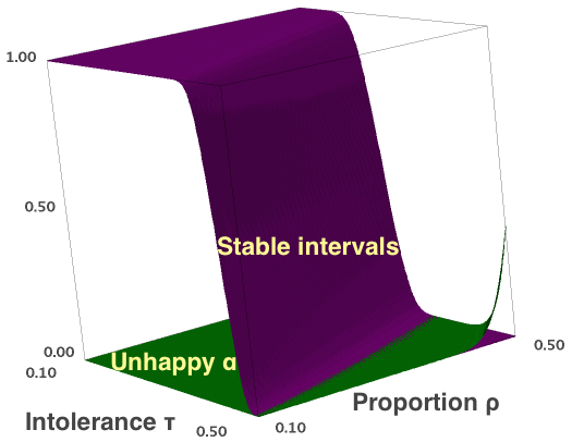
The values of for which we show that the process is static, correspond to the yellow area of the first diagram (or, equivalently, the collapsed part of the surface of the third diagram) of Figure 2. The case when presents a remarkable contrast as crosses the boundary of . In this case, when exceeds the threshold , the process changes from static to the other extreme of complete segregation.
Case Condition Happy Happy Balanced happiness , Unbalanced happiness ,
Corollary 1.3 (Phase transition on ).
If , then with high probability the process
- •
converges to complete segregation if ;
- •
is static, if .
Moreover with high probability it reaches its final state in time , if and time , if .
We display these results in the second item of Table 1. In Sections 2–4 we present the argument that proves these results. This argument uses a number of smaller results which are stated without proof, and are the building blocks of the proof of Theorem 1.2. It is our intention that the reader gets a fairly good understanding of our analysis in this part of the paper, without the burden of having to verify some of the more technical parts of the proof. Section 5 is an appendix with detailed proofs of all the facts that were used in Sections 2–4, and completes the proofs of Theorem 1.2 and Corollary 1.3.
Our proof of Theorem is nonuniform, and the analysis is roughly divided in the two cases displayed in Table 4: balanced and unbalanced happiness. Here happiness refers to the numbers of initially happy nodes of the two types, and determines the dynamics that drives the process to an equilibrium. Of the two cases, unbalanced happiness is the most challenging to deal with, and the dynamics is driven by small number of unhappy -nodes against the large number of unhappy -nodes, which in fact is preserved throughout a significant part of the process.
2 Metrics and reaching complete segregation
One of the most challenging problems in the analysis of the segregation process is the large number of absorbing states. In order to understand which transitions are possible, we use certain metrics that describe the current state.

2.1 Welfare, mixing, and expectations
We define global metrics that reflect the welfare of the entire population. An obvious choice is the number of happy nodes at a given state. It is not hard to devise transitions of the process which reduce the total number of happy nodes (see the second plot of Figure 5). However it is possible to show that if the total number of happy nodes is approximately non-decreasing (in the sense that it is for some nondecreasing function on the stages, where the underlying constant depends only on ). Let the utility of a node (at a certain state) be the number of nodes of the same type in its neighborhood. A better behaved global metric of welfare of a state is the sum of the utilities of the nodes in the state. We call this parameter the social welfare of the state and denote it by . A consequence of the transition rule and the definition of utility is that the social welfare does not decrease along the stages of the process. Furthermore, if , every transition of the process strictly increases the social welfare. Let the mixing index of a node be the number of nodes in its neighbourhood that are of different type. The mixing index mix of a state is the sum of the mixing indices of the -nodes in that state. The mixing index of a state is also equal to the sum of the mixing indices of the -nodes in that state. The relationship between the two metrics is
Hence the mixing index is non-increasing along the transitions. Note that a single swap cannot decrease the mixing index by more than . On the other hand, by linearity of expectation we can calculate that
| the expectation of the mixing index in the initial state of is . |
The mixing index of complete segregation (in nontrivial cases) is . Since , this means that (with high probability) the process can reach complete segregation only after stages, i.e. stages. On the other hand, a case analysis shows that if , each step in the process decreases the mixing index by at least 4. This means that if and the process is static, then it reaches its final state within stages. This happens because each time a swap occurs, the mixing index decreases by at least 4 (so its not possible that the same few nodes swap more than times). We have shown that the second clause of Corollary 1.3 (concerning the time to the final state) follows from the first clause.
As another measure of mixing, we may consider the number of maximal -blocks in the state. These are the contiguous -blocks that are maximal, in the sense that they cannot be extended to a larger contiguous -block. Let be the number of unhappy nodes in a state. It is not hard to show that if then and in particular
| (2.1.1) |
This means that the number of unhappy nodes at a certain state reflects the progress of the process towards segregation. More precisely, the metrics mix, , are mutually proportional when , where the analogy coefficient depends on (see Figure 5). In Table 3 we display these global metrics of welfare, along with their dynamics. A function (on the stages of the process) has positive dynamics if it is non-decreasing and approximately positive dynamics if it is for some nondecreasing function , where the multiplicative constant does not depend on . Similar definitions apply for ‘negative’. The first clause of Theorem 1.2 (the case when ) is the hardest to prove. It turns out that in this case we can deduce a non-trivial lower bound on the mixing index of dormant states.
Lemma 2.1 (Mixing in dormant states).
Consider the process with . The mixing index in a dormant state is more than , as long as .
The case is further divided in two cases, which reflect the proportions of happy nodes in the initial state. We display these in Table 4, along with the corresponding expectations for the numbers of happy nodes of each type. Lemma 2.1 is crucial for the proof of the first clause of Theorem 1.2 (in particular the case ).
2.2 Accessibility of dormant states and complete segregation
We show the case of Theorem 1.2 where and . This argument consists of two parts. First, we show that in this case with high probability the initial state is such that every state with the same number of -nodes has unhappy nodes of both types (i.e. it is not dormant). Hence under these conditions, no accessible state is dormant. The second part consists of showing that from every state there is a sequence of transitions to either a dormant state or complete segregation. Moreover the latter fact holds in general, for any values of , so it can be reused for the case when , in Section 3. This latter case is more challenging, as it can be seen that there are permutations of the initial state which are dormant.
Lemma 2.2 (Existence of unhappy nodes).
Suppose that , and is sufficiently large. Then for every and all sufficiently large , every state of the process has more than unhappy -nodes. If in addition , every state also has more than unhappy -nodes.
Given , by the law of large numbers with high probability (tending to 1, as tends to infinity) will be arbitrarily close to . Hence we may deduce the absence of dormant states (with high probability) in the case that .
Corollary 2.3 (Absence of dormant states when and ).
If and then with high probability none of the accessible states of the process is dormant.
It remains to show the accessibility of either a dormant state or complete segregation, from any state of the process. An inductive argument can be used in order to prove this fact.
Lemma 2.4 (Complete segregation or dormant state).
From any state of the process with there exists a series of transitions to complete segregation or to a dormant state.
Here is a sketch of the proof. If the mixing index is strictly decreasing through the transitions, so it is immediate that the process will reach a dormant state (indeed, 0 is a lower bound for the mixing index). For the case where (which we assume for the duration of this discussion) we can argue inductively, in four steps. An interval of nodes of the same type is called a contiguous block. First we show that from a stage with few unhappy nodes of one type (here is a convenient upper bound of what we mean by ‘few’, which is by no means optimal) there is a series of transitions which lead to either a state with a contiguous block of length or a dormant state. Second, from a state with a contiguous block of length there is a series of transitions to complete segregation or to a dormant state. Third, any state which has at least unhappy nodes of each type, there is a series of transitions to a state with a contiguous block of length at least . Finally from a state that has a contiguous block of length and at least unhappy nodes of opposite type from the block, there is a series of transitions to a state with a contiguous block of length . The combination of these four statements constitutes a strategy for arriving to a dormant state or a state of complete segregation, from any given state. We illustrate this strategy in Figure 6, where two arrows leaving a node indicate that at least one of these routes are possible.

3 Reaching complete segregation when and
This case of Theorem 1.2 is challenging because we need to show that the process avoids accessible dormant states, until it reaches a safe state i.e. a state from which no dormant state is accessible. The reason for this avoidance is (in contrast with the case of Section 2.2) the dynamics of the process with the given parameters. The methodology we use is based on a martingale argument, which involves a great deal of the analytical tools (e.g. the metrics of social welfare) and their properties that were developed in the previous sections. Having shown that dormant states are avoided until the process reaches a safe state, Lemma 2.4 gives Theorem 1.2 (for the case where and ). An overview of this argument is given in Figure 8.
3.1 The persistence of large contiguous -blocks
According to our plan, we wish to establish the existence of unhappy nodes of both types until a safe state is reached. By Lemma 2.2, we do not have to worry about the existence of unhappy -nodes. One device that guaranties the existence of unhappy -nodes is a contiguous block of -nodes, of length at least . Such a block exists in the initial random state (with high probability). One way to argue for its preservation in subsequent stages is to consider the ratio of the unhappy nodes of the two types. Even more relevant is the ratio between the number of unhappy -nodes, and the number of -nodes which are not just unhappy, but actually sufficiently unhappy that they can swap with any unhappy -node.
Definition 3.1 (Very unhappy -nodes).
Given a stage of the process, a node of type is very unhappy if there are at least nodes of type in its neighbourhood. The number of very unhappy -nodes is denoted by .
In the case that we study ( and ) initially, the number of very unhappy -nodes is while the number of unhappy -nodes is . The following lemma says that as long as this imbalance is preserved, it is very likely that a sufficiently long contiguous block of -nodes is preserved.
Lemma 3.2 (Persistent -block).
Consider the process with and let be the least stage where the ratio between the very unhappy -nodes and the unhappy -nodes becomes less than (putting if no such stage exists). Then with high probability there is a -block of length at all stages of the process.
Since a -block of length at least is a guarantee for unhappy -nodes, we get the following corollary.
Corollary 3.3 (Conditional existence of unhappy -nodes).
Under the hypotheses of Lemma 3.2, with high probability there are unhappy -nodes at all stages of the process.
It remains to construct an elaborate martingale argument in order to show that the imbalance between and persists for a sufficiently long time (until the process reaches a safe state).
3.2 Infected area view of the Schelling process
In the case of unbalanced happiness (i.e. when , , see Table 4) the unhappy -nodes are initially very rare, so the interesting activity (namely -to- swaps) occurs in small intervals of the entire population (at least in the early stages). These intervals contain the unhappy -nodes, and gradually expand, while outside these intervals all -nodes are very unhappy. Figure 11 shows the development of this process, where the height of the nodes (perpendicular lines) is proportional to the number of -nodes in their neighborhood and the horizontal black line denotes the threshold where an -node becomes unhappy. Hence nodes with high proportion of -nodes in their neighbourhood will be higher than the nodes with low proportion of -nodes in their neighbourhood. The three horizontal bars are snapshots of the process, and show cascades forming, originating from the initially unhappy -nodes. Figure 7 shows the same process, with the current state in the outer circle, and with swaps represented by a dot at a distance from the center which is proportional to the stage where the swap occurred. These cascades that spread the unhappy -nodes are due to the following domino effect. An unhappy -node moves out of a neighbourhood, thus reducing the number of -nodes in that interval. This in turn often makes another -node in the interval unhappy, which can move out at a latter stage, thus causing another -node nearby to be unhappy, and so on. The expanding intervals are the infected segments which start their life as incubators. For the sake of simplicity, we omit the formal definitions of these notions, which can be found in the appendix. Roughly speaking, incubators are a small intervals that surround the unhappy -nodes in the initial state. Moreover they are defined in such a way that, every -node that is outside the incubators is very unhappy in the initial state. During the process, as we discussed above, these expand into larger infected segments, so that at each stage every unhappy -node is inside an infected segment. The union of all infected segments is called the infected area. At any stage, every -node outside the infected area is very unhappy and every -node outside the infected area is happy. It is not hard to show that if , the probability that a node belongs to an incubator is . Hence with high probability the number of incubators as well as the number of nodes belonging to incubators of the process is .
It turns out that the number of unhappy -nodes in an interval of nodes, is conveniently bounded in terms of the number of -nodes in the interval. This means that if the number of -nodes in the infected area remains , then the number of unhappy -nodes in the infected area also remains . In order to give a clear sketch of the argument depicted in Figure 8 (for the current case when and ) let us define the global variables in Table 9 (for the current discussion we will not be concerned with or its definition). Note that Since . A combinatorial argument can be used in order to show that . Hence
| (3.2.1) |
By (2.1.1) we know that a stage where the number of unhappy nodes is less than is a safe stage. Hence we wish to show that (with high probability) the process will arrive at a stage where each of the three summands in (3.2.1) are at most . We know that can be bounded appropriately. Our main argument will show how to obtain a similar bound for . Note that plays a different role, since it is initially large and shrinks monotonically (as the infected area expands monotonically). In order to find a stage where becomes sufficiently small, it is instructive to consider what is a typical swap in the process. At the start of the process the infected area is a very small proportion of the entire ring. The vast majority of unhappy -nodes occur outside the infected area, while all unhappy -nodes are inside the infected area. It follows that with high probability a swap will involve an -node in the infected area and a -node outside the infected area. A bogus swap is a swap is one that is not of this kind.
Definition 3.4 (Bogus swaps).
A swap which involves a -node currently inside the infected area is called bogus. Given an infected segment , a bogus swap in is a swap that moves an -node into .
-nodes in infected area Unhappy -nodes in infected area Anomalous nodes in infected area Probability of a bogus swap -nodes outside infected area. Nodes inside the incubators
Note that any swap which is not bogus, reduces by at least 1. Hence if we show that the bogus swaps have small probability throughout a significant part of the process, we can ensure that becomes sufficiently small. In order to be more precise, recall the stopping time from Lemma 3.2. We introduce a few more stopping times, all of which will turn out to be earlier than (with high probability). These basically concern the satisfaction of conditions which will ensure that the mixing index is sufficiently low as to guarantee a safe state. By (2.1.1) we have and in order to ensure a safe state (by Lemma 2.1) we want . So we want at some stage of the process. Let be the first stage which satisfies this condition. Similarly, consider the stopping times of the second part of Table 3 (for simplicity, we will not consider in the present discussion). We use an elaborate martingale argument in order to show the following.
Lemma 3.5 (Bounding the -nodes in the infected area).
If and , with high probability we have and for all .
This lemma in combination with Corollary 3.2 implies that . Hence every stage up to involves a swap. Then it follows from the second clause of Lemma 3.5 that (since is reduced by at least 1 at every non-bogus swap). Hence by (3.2.1) we have established (with high probability) the existence of a stage such that
Hence by (2.1.1) we have , which means that by stage a safe state has been reached. Then by Corollary 2.4 the process will reach complete segregation, with probability .
Corollary 3.6 (Safe state arrival).
Suppose that . Then with high probability the process reaches a safe state by stage , and eventually complete segregation.
This argument (with the full details given in Section 5) concludes the proof of Theorem 1.2 for the case . It remains to deal with the case .
Property Probability Distribution Likelihood Stable -interval high if , low if Unhappy -node always rare
4 The case when intolerance is at most 50%
In this case the behaviour of the process is very different, since the mixing index is strictly decreasing. This means that the process is bound to arrive to a dormant state, with absolute certainty. Note that if then complete segregation is a dormant state, but it can be shown that the final state is never complete segregation. We show that in most typical cases for , the outcome is static when . We assume that because the case has already been analysed in [BIKK12, BELP14] and the case is symmetric. Hence on the hypothesis we have and by Table 4 the unhappy -nodes are an arbitrarily small proportion of the -nodes as . In any case, since we have , so the probability that an -node is unhappy is much smaller than the probability that a -node is unhappy. However what matters in the analysis for is the relationship between the likelihood of stable intervals and unhappy -nodes. This analysis is a reminiscent of the work in [BELP14], but has some new features.

Definition 4.1 (Stable intervals).
A stable interval is an interval of nodes of length which contains at least nodes of one or the other type. An interval is -stable if it contains at least nodes of type .
The -stable intervals are defined analogously. Note that no -node which is inside an -stable interval can swap during the process. The reason is that such -nodes are happy just because of the presence of the other -nodes in the same interval. Then a simple induction shows that they will continue to be happy throughout the process, thereby remaining immune to swaps and fixed in their initial positions. A similar observation applies to -stable intervals. The existence of stable intervals is characteristic to the case .
The events we are interested are the occurrences of -stable intervals and unhappy -nodes. The probabilities of these two rare events can be viewed as tails of certain binomial distributions. Consider the variables, probabilities and distributions of Table 10. It is not hard to see that
We are interested in the event where the ratio becomes small, because of the following fact.
Lemma 4.2 (Static processes).
Suppose that are such that for some . Then with high probability the process is static, and in fact there exists some such that with high probability the process stops after at most many steps.
Threshold Solution to equation Stability condition and and
The intuition here is that, if the unhappy -nodes are much more rare than the stable -stable intervals (i.e. if ) then it is very likely that unhappy -nodes are enclosed in small intervals which are guarded by -stable intervlas. This means that the familiar cascades that can be caused by the eviction of an unhappy -node are bound to be contained in small areas of nodes. The very definition of stable intervals ensures that such cascades cannot pass through them. Hence the condition guarantees that any -to- swaps are contained in small areas of nodes of total size . Due to the monotonicity of the mixing index, this means that there can only be at most swaps in this case.
The second item in Figure 2 shows the probabilities (for ) with respect to . We see that for points away from , the surface is above , and there is a threshold curve beyond which the opposite relationship is established. Using basic results about the tail of the binomial distribution, and Stirling’s approximation we can derive the following sufficient condition for :
| , where | (4.0.1) |
The third item of Figure 2 is a representation of in the space, up to where it becomes negative, at which point we project it on the plane. The values of that we are interested correspond to points on the plane, outside the collapsed area. This boundary (a curve) is more clear in the first item of Figure 2 which is the projection of the surface to the plane, with different colours indicating the points which make positive or negative. This boundary can be simplified (with slight loss of generality) if we consider the line that passes from the two points where the boundary curve intersects the lines and . Hence if , we are in the stable region, which shows a clause of Theorem 1.2. Note that both of the partial derivatives of are negative when . If we fix then the largest value of that keeps is the solution () of the first equation of Table 12. Hence we may conclude that if and then for some . We can also look for the largest square that is contained in the large area of the first item of Figure 2 (where the process is static). The edge of this square is given in Table 12. Hence if then for some .
We have one last observation to make about the function . If we let do not restrict the values of then we wish to find the values of such that . According to the properties of (in particular its negative derivative on ), these are all the positive numbers which are less than the limit (which is also an infimum)
Hence we may conclude that if and then for some . This concludes the proof of the second clause of Theorem 1.2.
References
- [BELP14] G. Barmpalias, R. Elwes, and A. Lewis-Pye. Digital morphogenesis via Schelling segregation. In 55th Annual IEEE Symposium on Foundations of Computer Science, Oct. 18-21, Philadelphia, 2014. FOCS 2014.
- [BELP15] G. Barmpalias, R. Elwes, and A. Lewis-Pye. Tipping Points in 1-Dimensional Schelling Models with Switching Agents. J. Stat. Phys., 158:806–852, 2015.
- [Ber12] E. Bertin. A Concise Introduction to the Statistical Physics of Complex Systems. Springer Briefs in Complexity. Springer, Springer Berlin Heidelberg, 2012.
- [BIKK12] C. Brandt, N. Immorlica, G. Kamath, and R. Kleinberg. An analysis of one-dimensional Schelling segregation. In STOC ’12: Proceedings of the 44th symposium on Theory of Computing, pages 789–804, 2012.
- [BMR14] P. Bhakta, S. Miracle, and D. Randall. Clustering and mixing times for segregation models on . In Proceedings of the Twenty-Fifth Annual ACM-SIAM Symposium on Discrete Algorithms, SODA 2014, Portland, Oregon, USA, January 5-7, 2014, pages 327–340, 2014.
- [Bolon] B. Bollobás. Random Graphs. Cambridge Studies in Advanced Mathematics 73. Cambridge University Press, Trinity College, Cambridge and University of Memphis, 2001, Second Edition.
- [CACP07] R. Conte, G. Andrighetto, M. Campennì, and M. Paolucci. Emergent and immergent effects in complex social systems. In Proceedings of AAAI Symposium, Social and Organizational Aspects of Intelligence, Washington DC, 2007. Association for the Advancement of Artificial Intelligence.
- [CF08] W. Clark and M. Fossett. Understanding the social context of the Schelling segregation model. Proceedings of the National Academy of Sciences, 11:4109–4114, 2008. col. 105.
- [CFL09] C. Castellano, S. Fortunato, and V. Loreto. Statistical physics of social dynamics. Reviews of Modern Physics, 81:591–646, 2009.
- [Cla91] W. Clark. Residential preferences and neighborhood racial segregation: A test of the Schelling segregation model. Demography, 28:1–19, 1991.
- [CM11] P. Collard and S. Mesmoudi. How to prevent intolerant agents from high segregation? In Advances in Artificial Life (ECAL 2011), Paris, France (T. Lenaerts et al., eds.), Cambridge, MA: MIT Press, 2011.
- [CMGP13] P. Collard, S. Mesmoudi, T. Ghetiu, and F. Polack. Emergence of frontiers in networked Schelling segregationist models. Journal of Complex Systems, 22, 2013.
- [DCM08] L. Dall’Asta, C. Castellano, and M. Marsili. Statistical physics of the Schelling model of segregation. Journal of Statistical Mechanics: Theory and Experiment, 7, 2008.
- [dSGL07] Michael J. de Smith, Michael F. Goodchild, and Paul A. Longley. Geospatial Analysis: A Comprehensive Guide to Principles, Techniques and Software Tools. Troubador Publishing, 2nd edition, 2007.
- [EA96] J.M. Epstein and R. Axtell. Growing Artificial Societies: Social Science from the Bottom Up. A Bradford book. Brookings Institution Press, 1996.
- [Fos06] M. Fossett. Ethnic preferences, social distance dynamics, and residential segregation: Theoretical explorations using simulation analysis. Journal of Mathematical Sociology, 30:185–273, 2006.
- [GB02] N. Gilbert and S. Bankes. Platforms and methods for agent-based modeling. Proceedings of the National Academy of Sciences, 99(suppl 3):7197–7198, 2002.
- [Hay13] B. Hayes. The math of segregation. American Scientist, 101(5):338–341, 2013.
- [HCSB11] A.J. Heppenstall, A.T. Crooks, L.M. See, and M. Batty. Agent-Based Models of Geographical Systems. Springer Netherlands, 2011.
- [LG09] J.-P. Nadal L. Gauvin, J. Vannemenus. Phase diagram of a Schelling segregation model. European Physical Journal B, 70:293–304, 2009.
- [Mou10] Nima Mousavi. How tight is Chernoff bound?, 2010. Draft which is available for download at http://ece.uwaterloo.ca/nmousavi.
- [Ó08] G. Ódor. Self-organising, two temperature Ising model describing human segregation. International journal of modern physics C, 3:393–398, 2008.
- [PW01] M. Pollicott and H. Weiss. The dynamics of Schelling-type segregation models and a non-linear graph Laplacian variational problem. Adv. Appl. Math., 27:17–40, 2001.
- [Sch69] T. C. Schelling. Models of segregation. The American Economic Review, 59(2):488–493, 1969.
- [Sch71a] T.C. Schelling. Dynamic models of segregation. Journal of Mathematical Sociology, 2:143–186, 1971.
- [Sch71b] T.C. Schelling. On the ecology of micromotives. The Public Interest, 25:61–98, 1971.
- [Sch78] T. C. Schelling. Micromotives and Macrobehavior. New York, Norton, 1978.
- [Sch07] M.C. Schut. Scientific handbook for simulation of collective intelligence. http://www.sci-sci.org, 2007.
- [Slu77] E. V. Slud. Distribution inequalities for the binomial law. Ann. Probab., 5:404–412, 1977.
- [SS07] D. Stauffer and S. Solomon. Ising, Schelling and self-organising segregation. The European Physical Journal B - Condensed Matter and Complex Systems, 57(4):473–479, 2007.
- [SSD00] R. Sander, D. Schreiber, and J. Doherty. Empirically testing a computational model: The example of housing segregation. In Proceedings of the Workshop on Simulation of Social Agents: Architectures and Institutions, pages 108–115, Lexington, MA, 2000. Lexington Books.
- [Wil99] U. Wilensky. NetLogo Models Library: Sample Models/Social Science. NetLogo. http://ccl.northwestern.edu/netlogo, Center for Connected Learning and Computer-Based Modelling, North-Western University. Evanston, IL., 1999.
- [YÖ09] L. Yilmaz and T. Ören. Agent-Directed Simulation and Systems Engineering. Wiley Series in Systems Engineering and Management. Wiley, 2009.
- [You98] H.P. Young. Individual Strategy and Social Structure: An Evolutionary Theory of Institutions. Princeton University Press, Princeton, NJ, 1998.
- [Zha04a] J. Zhang. A dynamic model of residential segregation. Journal of Mathematical Sociology, 28(3):147–170, 2004.
- [Zha04b] J. Zhang. Residential segregation in an all-integrationist world. Journal of Economic Behavior & Organization, 54(4):533–550, 2004.
- [Zha11] J. Zhang. Tipping and residential segregation: A unified Schelling model. Journal of Regional Science, 51:167–193, 2011.
5 Appendix
In this section we provide supplementary material to the main part of the paper. This includes mainly proofs of the claims we made towards the proof of our main theorem, but also additional introductory material, figures, tables and mathematical background. The structure of this supporting material follows the presentation of the main part of the paper.
5.1 Schelling models
The definition of the Schelling model in Section 1.1 is rather standard, close to the spacial proximity model from [Sch69, Sch71a] and identical to the model studied in [BIKK12, BELP14]. Most significantly, it is an unperturbed Schelling model, where agents cannot make moves that are detrimental to their welfare. We have already remarked in the introduction that various more realistic-looking rigorously analysed perturbed versions of the model in the literature (such as [Zha04a]) actually force ‘regularity’ on the process, which makes it fit an already existing methodology (such as Markov chains with a unique stationary distribution, or with properties that guarantee stochastically stable states). Even if we commit to the absence of perturbations in the model, it is possible to add complications to the simple dynamics defined in Section 1.1. For example, the agents may take into account the distance they need to travel before they move. However it is the simplicity of the original Schelling model, contrasted by the complexity of the analysis required to specify its behaviour (as demonstrated in [BIKK12, BELP14]) that make this topic fundamental and interesting.
Under the above requirement for simplicity and proximity to the original model, there remain a number of ways that the model can be altered or generalised. For example, note that in the case that in the model of Section 1.1, two nodes may swap although the number of same-type nodes in their neighbourhoods remain the same after the swap. One may alternatively require that for such a swap, the corresponding numbers of same-type nodes in the neighbourhoods increase (note that such a modification would not make a difference if ). Our choice on this issue follows Brandt, Immorlica, Kamath, and Kleinberg in [BIKK12, Section 2]. One generalisation, considered in [BELP15], is to allow different tolerance thresholds for the two types of individuals. Another generalization, already present in [Sch69], is to introduce a number of vacancies, i.e. to allow the total number of individuals to be smaller than the number of sites. We could also alter the dynamics. Instead of switching two chosen individuals at each stage, we could merely choose one individual and change his type. Such an action may be interpreted as the departure of the individual to some external location and the arrival of an individual of the opposite type at the site that has just become available. Model with this dynamics are often said to have switching agents (see [BELP15], where such a model was analysed) as opposed to the swapping agents of the model of Section 1.1.
It is worth pointing out that the Schelling model with switching agents is closely related to the spin-1 models used to analyse phase transitions in physics, and in particular the Ising model. Indeed, in the Ising model (originally introduced in order to explain ferromagnetism in the context of temperature) a system of atomic nuclei interact with an auxiliary ‘heat bath’ which affects their spin. Such connections have been analysed by many authors (see for example [SS07, DCM08, PW01, LG09, Ó08]), where the dynamics is based on the Boltzmann distribution on the set of possible configurations. A rough analogy between the two models is that ‘energy’ corresponds to some measure of the mixing of types (see the definition of the mixing index for the Schelling model below) and ‘temperature’ corresponds to the intolerance parameter (as least insofar phase transitions refer to varying values of the temperature or ). On the other hand, the Schelling model with closed dynamics has a counterpart in the Ising model with Kawasaki dynamics.
5.2 Objectives of the analysis of the unperturbed model and related work
We use the notation of Section 1.1, so that the symbol always means the population variable of the process, and always is the parameter of the process which determines the length of the neighbourhood of nodes. Similarly, always refer to the parameters of the Schelling process.
In Section 5.12 we show that, with probability one, the process either reaches complete segregation or it reaches a dormant state. In the second case, we wish to determine the extent of segregation in the dormant state. In view of the large number of states that the process may have (most of them ‘random’) a question arrises as to how to classify or even talk precisely about different states that may be the outcome of the process. Brandt, Immorlica, Kamath, and Kleinberg noticed in [BIKK12] that, at least in the case that they considered, the extent of the segregation that occurs in the final state depends crucially on . In fact, they showed that the dependence on is ‘polynomial’. We may say that a state is regarded as polynomial segregation if, with high probability a randomly chosen node belongs to a contiguous block of size that is proportional to the value of a polynomial on . A similar definition applies to exponential segregation. These two notions turn out to provide a very useful language for explaining the eventual outcome of the Schelling process. A full characterization (extending the work of Brandt, Immorlica, Kamath, and Kleinberg [BIKK12]) of the asymptotic behaviour of the process for and was provided by the authors in [BELP14] in terms of polynomial and exponential segregation, as well as static processes. Intuitively, a random state is non-segregated, while polynomial and exponential segregation correspond to highly non-random states.
Intolerance Segregation Negligible Exponential Polynomial Complete
The characterization from [BELP14] is summarized in Table 13. It is rather striking that when intolerance is increased from, say, to the segregation is decreased. This phenomenon is akin to the many paradoxes that stem from the missing link between local motives of agents and global behaviour of a system (e.g. see Schelling’s classic monograph [Sch78], and in particular Chapter 4 which relates to his segregation models). Even more strikingly, the authors showed in [BELP14] that the paradox occurs for all , i.e. as approaches the segregation (in the final state) decreases.
This paradoxical phenomenon is also clear in many simulations of the model. Figure 14 shows typical runs of the processes for . The final state is depicted in the circle, where the nodes of one type are black and the nodes of the other type are grey. We use the space between the centre of the ring and the ring in order to record the actual process, as it evolves in time. In particular, if a grey node switches its place with a black node, we put a black node (the colour of the more recent node) between the location of the node and the centre of the ring, at a distance from the centre which is proportional to the stage where the swap occurred. Hence we may observe “cascades’ of swaps of nodes of the same type, which are less severe as approaches . Such cascades are crucial in the rigorous analysis of the model, both in [BIKK12] and in [BELP14]. Figure 14 shows that as approaches , the segregation is decreased. This behaviour can be traced to the probability that a node is unhappy in the initial configuration, and in fact, the threshold constant is derived by comparing related probabilities in [BELP14].
In the case the two constants and mark phase transitions in the limit state of the process , as takes values in . This brings us to another important objective of the analysis of the Schelling process, which is the discovery of phase transitions with respect to the parameters . Incidentally, we note that the discovery of phase transitions has been one of the original motivations for the study of the one and two dimensional Ising model, when one varies the temperature (see the end of Section 5.1 for a brief discussion of the analogy between the Ising and the Schelling models). Finally we are also interested in the expected time that the process take to converge.

5.3 Asymptotic notation
We use the asymptotic notation. Given two functions on the positive integers, (as is standard) we say that is if there exists a positive constant such that for all . We say that is if is , and that is if both is and is . We also use this notation, however, in a more general sense: we say that is if there exists some such that for all . For example, when we say that a function is , this means that there is such that for all . Or, if we say that is , this means that there is such that for all . Similarly, we use in a more general sense. We say that is to mean that there exist constants and such that for all . We say that if . The (often hidden) variable underlying the asymptotic notation in the various expressions will be . In other words, for fixed values of and , the choice of constants required in the asymptotic notation, will always depend only on . We also combine the ‘high probability’ terminology with the asymptotic notation in a manner which is worth clarifying. When we say, for example, that ‘with high probability the number of initially unhappy -nodes in the process is ’, this means that there exist constants and such that, with high probability, the number of initially unhappy -nodes in the process lies between and .
5.4 Overview of our analysis
We use different methods for the cases and . If , in order to derive conditions under which the process is static, we analyse and compare the probabilities of initially unhappy nodes and stable intervals. This approach was introduced by the authors in [BELP14]. If we consider the two cases and and argue (using distinct arguments) that in each of them complete segregation is the high probability outcome. We elaborate on these arguments.
Case
This case is divided to the cases and , and the structure of the analysis was depicted as a flowchart in Figure 8. Here we give a more detailed overview, which is illustrated in the more elaborate flowchart of Figure 15. First, we show that asymptotically (on ), from any state there is a series of transitions that leads to either a dormant state, or complete segregation. Hence, since there are only finitely many states, with probability one the process will reach either a dormant state or complete segregation. So in order to establish complete segregation as the eventual outcome, it suffices to show that the process maintains unhappy nodes of each colour during all stages.
First, assume that . In this case we can show that, assuming that the actual proportion of -nodes is sufficiently close to (which is very likely according to the law of large numbers), every reachable state is not dormant. More precisely, we show that given such numbers of and -nodes, every permutation of them on the ring corresponds to a state which has both unhappy and unhappy -nodes. Since the numbers of nodes of each type do not change during each transition, this argument suffices for this case. Recall that states with the property that no series of transitions from them leads to dormant states are called safe. So, in the case we argue that (with high probability) the initial state is safe.
Second, we assume that , which is a considerably harder case. Under this hypothesis, in the initial configuration we have many unhappy -nodes and many unhappy -nodes. As before, it suffices to show that (with high probability) the process never reaches a dormant state. It is not hard to see that (with high probability) the initial state is not dormant. However it is no longer clear if the initial state is safe. We show that given the expected numbers of nodes of the two types in the initial state (or numbers sufficiently close to their expectations) any permutation of the nodes on a ring corresponds to a state with at least one unhappy -node. Hence, with high probability, the process will never run-out of unhappy -nodes and we only need to argue about the preservation of unhappy -nodes. Already it should be clear that this is an asymmetric case where the -nodes (the majority) and the -nodes (the minority) play different roles. When there are many permutations of the nodes (which correspond to states where all -nodes are happy, i.e. dormant states. So the argument that was used in the case is no longer relevant for arguing for the preservation of unhappy -nodes in the process. The argument we use instead is based on the asymmetry between the number of unhappy -nodes and the unhappy -nodes, which creates a dynamic that favours the preservation of unhappy -nodes. More precisely, it favours the preservation of -blocks of length , which is a condition implying the existence of unhappy -nodes (indeed, the -nodes neighbouring a -block of length at least are unhappy). Hence if we show that the expected number of unhappy -nodes remains small during the stages of the process, then we have that we can expect the existence of unhappy -nodes (and unhappy -nodes) up to the point where the total number of unhappy nodes is small.
In addition we show that if the total number of unhappy nodes in a state is sufficiently small, then this state is safe, i.e. there is no series of transitions from it to a dormant state. The argument is concluded by showing that it is very likely that by stage the process will arrive at a state with appropriately low number of unhappy nodes, before it reaches a dormant stage. Figure 5 is a plot of the numbers of unhappy -nodes and the unhappy -node during the stages, taken from two typical simulations (one with large and one with small population), when . The process we described is clearly visible: the number of unhappy -nodes remains small, until the number of unhappy -nodes becomes small. Up to the later point, as we explained, the dynamics favours the preservation of unhappy -nodes.
Case
In this case we have , and this means that in the initial configuration the -population is happy with a few exceptions, while the -population is unhappy, with a few exceptions. By the definition of the dynamics of the model -to- swaps can only occur in areas where there are unhappy -nodes. Hence in this case the -to- swaps will be concentrated in a very few selected areas in the ring, at least in the first stages of the process. This concentration of -to- swaps creates cascades of -node evictions which can be clearly seen in simulations such us the one displayed in Figure 7.22 2 Here the current configuration is the outer circle, while the initial random state is the inner small circle. Whenever a swap occurs at some stage, a dot is placed at a distance from the center which is proportional to that stage, at the same angle where the involved node lies. The color of the dot corresponds to the type that the node changed to under the particular swap. If we could argue that such cascades are restricted to small areas around the initially unhappy -nodes, then it is not hard to argue that the process reaches a dormant state rather quickly, having affected only a very small number of nodes. The way we do this is through stable intervals, a device that was also used in [BELP14]. Roughly speaking, these are intervals that do not allow the spread of unhappy -nodes through them.
If is very small, or if is very small, then stable intervals occur with high probability. On the other hand, if get sufficiently large, the probability of a stable interval tends to 0 as . This contrasts with prevalence of unhappy -nodes. When are small, the probability of (the occurrence of) an unhappy -node is small, while it gets large when increase. Figure 16 shows the actual probabilities (as calculated in Section 4) as functions of for the specific value of (the shape of the plots does not change significantly for different values of ). The interesting case is the range for where both probabilities tend to as , i.e. both events become rare. Somewhere on the horizontal - plane there is a line marking the intersection of the two surfaces. This is where the probability of a stable interval becomes less than the probability of an unhappy -node. Moreover, as the ratio of the two probabilities tends to infinity or zero, depending whether sit on one side of the plain (with respect to the intersection line) or the other. The crux of the argument in Section 4 is that for many values of stable intervals are much more common than unhappy -nodes in the initial configuration. This allows us to argue that, in this case, the process has to reach a dormant state after many swaps.

5.5 Properties of welfare metrics
The social welfare V of the state can easily be seen to be non-decreasing along the transitions of the process. Let us establish the relationship with the mixing index. Given a certain state of the process and a node , we let denote the number of nodes that are located in the neighbourhood of at this state. Similarly, we let denote the number of -nodes that are located in the neighbourhood of . Furthermore, we denote by and and the finite sequences of and nodes respectively in the state. Hence denotes the number of -nodes that are located in the neighbourhood of while denotes the number of -nodes that are located in the neighbourhood of . Given a state, let be the number of and -nodes respectively. Then
| (5.5.1) |
In order to prove this equality, consider the state of and types in the state and start by removing all from their positions. Then, adding the types one-by-one back to their original positions we can see each placement incurs the same increase to the two sums. Hence by induction, the two sums are equal.
We call the number in (5.5.1) the mixing index of the state, because it can be used as a metric of how mixed (i.e. not segregated) the population of and types is at the given state. Indeed, suppose that the state has at least nodes of each type. In the state of complete segregation the sums in (5.5.1) take the value , which is . This can be shown to be the minimum mixing index (in a state which has at least nodes of each type). At the other extreme, if the two types are uniformly mixed (in the sense that every interval has approximately green nodes) then the sums in (5.5.1) take approximately the value , which can be shown to be the maximum possible mixing index. We also have
| (5.5.2) |
Lemma 5.1.
If , each step in the process decreases the mixing index by at least 4.
Proof..
Suppose that we swap an unhappy -node with an unhappy -node . Let be the neighbourhoods of respectively and let . Here we view the nodes as stationary, so that a swap of nodes means a swap of their types. The mixing index of the nodes in will not change after the swap. Since the number of -nodes in is smaller the the number of -nodes in . After the swap the mixing index of each of the -nodes in will increase by one while the mixing index of each of the -nodes in the same set will decrease by one. If is the length of the neighbourhood and is the number of -nodes in then the mixing index of before and after the swap is (the size of the neighbourhood minus the -nodes in the neighbourhood) and (the number of -nodes in plus the number of -nodes in ) respectively. Hence the difference in the sum of the mixing indices of the nodes in before and after the swap is the addition of
- (a)
the difference in the mixing index of
- (b)
the difference in the sum of the mixing indices of the nodes in
where the differences refer to the stages before and after the swap. For (a) we have . For (b) there is an increase (by 1) of the mixing indices of each -node in since becomes a -node. Moreover there is a decrease (by 1) of the mixing index of the -nodes (as ceased to be an -node). Hence for (b) we have . Overall, the difference in the sum of the mixing indices of the nodes in before and after the swap is . A similar argument shows that the difference in the sum of the mixing indices of nodes in is . Hence overall (and since the nodes outside maintain the same mixing index before and after the swap) the difference in the (total) mixing index is . Since this means that a decrease by at least 4 occurs due to the swap. ∎
In our analysis, one of the basic facts used is that that dormant states have at least a reasonably high mixing index. If we can show that with high probability the process reaches a point where the mixing index is too low for dormant states to be accessible, then by Corollary 5.26 we will have shown that with high probability complete segregation is the eventual outcome. Proposition 5.3 below provides an appropriate bound for the mixing index of dormant states. First we prove a technical lemma, which will then be used in the proof of Proposition 5.3.
Lemma 5.2.
Suppose that , , and . In a dormant state of the process every -block has length at most and every -node is -near to an -node.
Proof..
Since the second claim implies the first, it suffices to prove the second claim. By Lemma 5.20 we can assume that there are unhappy -nodes in the given state. For a contradiction, suppose that some -node is not -near to any -node. Consider the -node which is adjacent to the block and to the right of it. For large , , meaning that this -node has at least nodes of type in its neighbourhood. Hence the -node has at most nodes of type in its neighbourhood, which is less than . The fact that this node is unhappy means that the state is not dormant. ∎
Proposition 5.3 (Mixing in dormant states).
Suppose that , , and . The mixing index in a dormant state of the process is more than .
Proof..
Suppose that in a dormant state the mixing index is at most . Since there are nodes of type , there exists such a node with mixing index at most . By Lemma 5.2 there exists an -node within nodes to the left or to the right of . The number of -nodes in the neighbourhood of is therefore at most . However this same number must be at least since is happy in a dormant state. This holding for arbitrarily large would imply that which gives the required contradiction. ∎
5.6 Number of unhappy nodes and maximal blocks
While a low mixing index suffices to establish the inaccessibility of dormant states, in fact it will often be more convenient to work directly with the number of unhappy nodes. The aim of this subsection is to allow us to do this, by establishing a fairly tight relationship between the number of unhappy nodes and the mixing index.
As another measure of mixing, we may consider the number of maximal contiguous -blocks in the state. Let be the th node of type and let denote the number of -nodes in the neighbourhood around . Let be a finite interval of integers such that constitutes a block (i.e. there is no -node between and ). If then is bounded above by . If the number continues to be a bound for . Therefore
| (5.6.1) |
This inequality is a formal expression of the rather obvious fact that the fewer maximal -blocks there are, the less mixed the two types are. By the definition of happy nodes, if and then no two adjacent nodes of different types can both be happy. This means that, as we move around the circle of nodes, every time we cross the border between a maximal -block and a maximal -block we may count an additional unhappy node. So, provided that and is sufficiently large, the number of maximal -blocks is bounded above by the number of unhappy nodes in the state. Then by (5.6.1) we get
Intuitively this inequality says that the only way to have a small number of unhappy nodes is a small mixing index, i.e. a large degree of segregation. On the other hand we may bound the number of unhappy nodes in terms of the mixing index. By (5.5.1) and the definition of unhappy nodes
where are the numbers of unhappy nodes of type and respectively. So
and
which means that if (and is sufficiently large) then .
5.7 Background on probability
We make use of the various concentration of measure inequalities for random variables and (super)martingales. The simplest of these is Markov’s inequality, which says that if is a non-negative random variable with and then . Recall Hoeffding’s inequality for independent Bernoulli trials.
Lemma 5.4 (Tight Hoeffding for Bernoulli variables).
Let be independent Bernoulli trials with expected value , and let . Then and for each . If then for each such that .
The second clause of this lemma (the tightness of the inequality) follows from Slud’s inequality [Slu77] (which gives a lower bound of the binomial upper tail in terms of the upper tail of the normal distribution) and standard lower bounds for upper tail of the normal distribution (see [Mou10] for more details).
Since there are complex dependences amongst the random variables of the Schelling process, we often need to ‘approximate’ certain processes with canonical processes like simple random walks. Here a random walk with respect to the integer-valued random variables is the stochastic process , for some . We say that is ruined at step if is the least number such that . The following simple fact is obtained via a standard coupling argument.
Lemma 5.5 (Random walk simulation).
Let , be (possibly dependent) random variables, let be independent Bernoulli trials and let , be the associated random walks. Provided that, no matter what occurs at stages prior to , at stage we have and , then for all the probability that is ruined by step is bounded above by the probability that is ruined by step .
The following fact about biased random walks is folklore.
Lemma 5.6 (Biased random walks).
Let , and let be (possibly dependent) random variables such that at stage , no matter what has occurred at previous stages, for some . Let , be the associated random walk. Then the probability that is ever ruined is bounded above by .
Proof..
Let be independent variables such that . Let be the associated random walk. Then , so by Lemma 5.5 it suffices to show that the probability that is ruined is bounded above by .
We may view as independent Bernoulli trials, where is viewed as success and is viewed as failure. Let , so . If is the number of successes up to step , then so ruin of the random walk at step implies that . We may use Lemma 5.4 in order to bound the probability of this event. If we let note that , so by Lemma 5.4, is an upper bound for the probability that is ruined at step . Next, note that can only be ruined at stages . Hence
is an upper bound of the probability that is ever ruined (before stage ), which concludes the proof. ∎
Our analysis depends on various exponential bounds that we can obtained on the expectations of certain parameters (e.g. the number of unhappy -nodes). The following fact will be routinely used in order to express such bounds in a canonical form. In the following statement the variables concern stage of the Schelling process and the constants are independent of .
Lemma 5.7 (Expectation bounds).
Let be a polynomial, and a random variables such that for all . If for some and all all and all sufficiently large then there exists such that for all .
Proof..
Since is a polynomial, we can choose and such that for all . Hence for all and all . We may choose such that for all . Then by the assumption on we have that for all and all . ∎
The binomial distribution with trials and success probability is denoted by , and means that random variable follows this distribution. Stirling’s formula asserts that , i.e. that the limit of the ratio of the two expressions tends to 1 as tends to infinity.
Lemma 5.8 (Stirling’s approximation).
There exists a polynomial such that for all and all
Proof..
Let or . Also let or . Then according to the definition of the binomial coefficient it suffices to show that there exists a polynomial such that
Note that there exists such that . Then
The second term on the right side of the equation is bounded by a polynomial in while the third term is in . Hence there is a quadratic polynomial such that
By Stirling’s approximation it follows that there exists a quadratic polynomial such that for all , and as defined above there exists such that . This fact, along with the definition of the binomial coefficient, implies the required statement. ∎
In our analysis of the Schelling process for the case when we will need to compare the tails of different binomial distributions. There are a number of ways for doing this (including using approximations with the normal distribution) but the simplest is the following elementary fact from [Bolon, Theorem 1.1].
Lemma 5.9 (Tails of the binomial distribution).
Suppose that , and for all sufficiently large , , where . Then
for all sufficiently large . In asymptotic notation we have .
The combination of this result with Stirling’s approximation of the binomial coefficients gives the required information about the asymptotic behaviour of the ratio of the two binomial probabilities of interest (unhappy nodes and stable intervals).
5.8 Martingales in the Schelling process
A crucial part of our analysis is based on two supermartingales, one regarding the non-anomalous -nodes in the infected area, and one regarding the anomalous nodes. The latter is somewhat sophisticated, in the sense that it is not adapted to the stages of the process. Nevertheless it is a supermartingale relative to a more general process, and this is sufficient for our analysis. Due to this sophistication, we clarify how we regard the process in probabilistic terms, and what we mean by a martingale.
The states of the system are all configurations of nodes that can have one or the other type. A state is accessible from another state (thought as an arrow from to ) if an application of a legitimate swap on gives . We view the random process as a combination of two parts. The first is the production of the initial state according to the given probability distribution of the two types. The second is the stochastic process that starts from the initial state and moves to the next state, choosing uniformly randomly from all the (finitely many) currently accessible states. We denote the initial state by and the state at stage by . The remaining discussion refers to the second part of the process, where is a constant. The underlying probability space is the set of all infinite sequences of states, which start with and have the property that each term is a state which is accessible from its predecessor. We also add into the finite sequences of states, which start with , each of their terms is accessible from its predecessor, and its last term is an absorbing state. We view this as a tree, where the th level of the tree (prefixes of points in the space of length ) describes all possible outcomes of the process up to stage . This tree has dead-ends, namely the absorbing states. The probability measure on is the uniform one, namely the one induced by splitting the total measure uniformly inductively starting from the route and considering all accessible paths. Then each can be viewed as random variable on , which takes any point in the space and outputs its th term.
A number of other processes will be defined, relative to the process which contains all the information. Clearly is memoryless (has the Markov property) since the distribution of only depends on the value of . The secondary processes that we consider in our analysis (like or ) can be seen as recording only part of the information of the full process up to stage . In general, a process is adapted to (or defined in terms of) another process if there is a function such that for every point in . Recall that a filtration on is an increasing sequence of -algebras on . The reader who is used to working with filtrations (especially with respect to martingales) can equivalently view a process adapted to another process as adapted to the natural filtration of : this is the filtration generated by the inverse images of the Borel sets of , with respect to the variables . For example, the natural filtration of the full process is where is the -algebra generated from the maximal branches of restricted to strings of length or less. Intuitively can measure all events that can possibly happen up to stage .
In order to show that a certain process is a martingale, we will have to adapt to another suitable process. Equivalently, we would have to adapt it to a suitable filtration (which may be different than the standard filtration that we described above). This is the reason for introducing adapted processes: the simplest martingale notion corresponds to processes adapted to themselves, and is not sufficient for our proof. Recall that a process is a supermartingale relative to a Markov process if it is adapted to it and for all . This means that relative to the set of reals in which have the particular value of (which is regarded as fixed) the expectation of is bounded by (which is a function of ). This is the standard definition of conditional expectation in terms of processes. In our analysis we occasionally need to consider conditional on a set of reals . We denote this by . A stopping time with respect to a process ) is a random variable such that the truth of the event (for any integer ) is a function of . If is a stopping time for and is a supermartingale with respect to , then the stopped process (which proceeds as up to stage , and then it is constantly equal to ) is also a supermartingale (with respect to ). Doob’s maximal inequality for supermartingales says that if is a non-negative supermartingale with respect to another process and , then .
5.9 Probability in Schelling segregation
In this section we lay out a general way for arguing about the probability of the various properties that a node can have in the initial configuration.
Definition 5.10 (Rare and common events in the initial configuration).
A property of a node in the initial configuration is called rare (or a rare event) if it holds with probability at most , for some positive constant which may depend on but not on . A property whose negation is rare is called common.
Definition 5.11 (Local properties).
A local property of a node in the initial configuration is one that only depends on the nodes that are at most -far from , where is a fixed function. In other words the property is local if given any two nodes such that for all , is of the same type as , then holds iff holds. In this case we say that is -local.
Note that the two probabilities mentioned in Lemma 5.12 are on different spaces. The first one refers to the product space where a point is an infinite series of initial states. The second one refers to the space of points on a random initial state.
Lemma 5.12 (Strong law of large numbers for the Schelling process).
Given a local property of nodes in the initial state of the process , with probability one, as the proportion of nodes that satisfy tends to the probability of .
Proof..
Let be the probability of and let be the function indicating the area around on which depends (as in Definition 5.11). We wish to use the strong law of large numbers, so we need to manufacture a series of independent trials of properties with given expectation. Let be a parameter that depends on (to be specified shortly). We consider the ring as a union of intervals of length (which we think of an interval of length with padding nodes on each side). We always assume that . Starting from node , denote the th such interval by so that . Also, denote the subinterval of that results from deleting the -node prefix and the -node suffix of by . Hence . Let be the largest integer such that , so that as and . Hence for each , the intervals are defined and are disjoint. The same is true for , . Moreover, if is the set of all nodes,
| (5.9.1) |
For each let be the number of nodes such that holds, and note that these random variables are independent. Moreover, by linearity of expectation, . Recall that as . According to the strong law of large numbers,
| (5.9.2) |
By (5.9.1), the required proportion is
where range in (depending on how close is to being a multiple of ). If we take , the ratio tends to , so by (5.9.2) the required proportion tends to
Since , the required proportion tends to . More formally, we may let . In this case, as we have because tends to . Moreover and when so the previous argument applies as indicated. ∎
The following fact concerns pairs of properties and that a node can have, which may both be rare but one (say ) occurs with much higher probability than the other. It asserts that in this case, a random node is much more likely to be nearer to a node satisfying than a node satisfying (although it may be far from any node satisfying or ). In the statement and proof of this result we use as a Boolean random variable which asserts that ‘ satisfies ’ (and similar with ).
Lemma 5.13 (Rare properties in the Schelling ring).
Let , be -local properties of nodes in the initial state (where is a function of ) and for each node let be the first node to the right of such that either or holds. If are the probabilities of respectively, the probability that and there is no node with to the left of and at distance at most from tends to a number as . An analogous result holds when ‘right’ is replaced by ‘left’.
Proof..
Consider a partition of the ring into disjoint neighbourhoods, starting from a node as follows. Recall that addition of nodes is always modulo . Given , suppose inductively that has been defined. Then define . This iteration continues as long as . Let be the number of iterations in this recursive definition (i.e. the number of terms of the sequence ). Consider the property
The sequence can be seen as independent trials for this property. Let be the proportion of the terms of that satisfy of in a random initial state. Note that as with probability 1. If is the probability of , by the strong law of large numbers we have that as with probability 1. Let be the proportion of nodes that satisfy and let be the proportion of nodes that satisfy . Note that we view as random variables that depend on the initial state. Then
By Lemma 5.12 we have and as , which gives the required assymptotic bound. ∎
5.10 Initial expectations
An important part of our analysis relies on the values of the welfare metrics at the initial state. With high probability, these will be near to their expected values, which we may compute. We start with the mixing index.
Lemma 5.14.
The expectation of the mixing index in the initial state of is .
Proof..
Consider the random variables and note that for each . If is the number of -nodes, the expectation of the mixing index in the initial state is by the linearity of expectation. If we see as a random variable, its expected value is . By the rule of iterated expectation, the expected value of the mixing index is . ∎
Note that the expected value of the mixing index in the initial state is only slightly smaller than the maximum possible mixing index . This is hardly surprising, as a random state will be almost perfectly mixed, with the occasional non-uniformities that are implied by randomness (e.g. the existence of contiguous blocks of certain sizes).
Next, we are interested in the expected number of unhappy nodes of each type. It is not hard to see that this depends on whether or (we will not consider the special case where ).
Lemma 5.15 (Unhappy -nodes).
Given such that , with high probability the number of initially unhappy -nodes in the process is .
Proof..
Let be 1 if the th node in the initial state is of type and unhappy, and 0 otherwise. By Lemma 5.12, it suffices to show that is . Recall that the nodes are labelled independently, following a Bernoulli distribution, with the probability of a -label being . Let which is positive, according to our hypothesis. If is an unhappy -node, then the proportion of -nodes in its neighbourhood is larger than . Hence the proportion of -nodes in is larger than , so it is at least .
Let be the event that is an -node and the event that is unhappy, so that and . If we see the labels of the nodes in as a series of independent Bernoulli trials, by Hoeffding’s inequality for Bernoulli trials the probability that the proportion of -nodes is at least is bounded by . Hence by the above discussion, . We may conclude that . Hence . Similarly, by Lemma 5.4 we have . Hence is , which concludes the proof. ∎
A similar argument gives an analogous result for the unhappy -nodes.
Lemma 5.16 (Unhappy -nodes).
Given such that , with high probability the number of initially happy -nodes in the process is . If in addition , with high probability this number is .
Proof..
Let be 1 if is of type and happy, and 0 otherwise. Then provided that , by Hoeffding’s inequality for Bernoulli variables we have that . Then Lemma 5.12 gives the first clause of the claim. Now lets assume that we also have . Then by the second clause of Lemma 5.4 we get . This application is possible with and because and , which means that . Then by Lemma 5.12 we get the second clause of the claim. ∎
By a similar argument we get a bound on the total size of the incubators.
Lemma 5.17 (Number of incubators).
If , the probability that a node belongs to an incubator is . Hence with high probability the number of incubators as well as the number of nodes belonging to incubators of the process is .
Proof..
Let , and let be the index variable of the event that the left semi-neighbourhood of the th node has less than many -nodes. Given that , by Hoeffding’s inequality for Bernoulli variables (Lemma 5.4) and the tightness of it (Lemma 5.4), the probability that is . Let be the index variable of the event that the th node belongs to an incubator, so that the probability that is (since is ). Hence is . Then by Lemma 5.12 with high probability the number of nodes belonging to incubators of the process is . ∎
5.11 Accessibility of dormant states
It is crucial to understand the dormant states and assess their accessibility from an initial state. IWe demonstrate that this issue ultimately depends on the given parameters . We show that if then with high probability we may assert that no dormant state is accessible from the initial state. On the other hand, if then with high probability there are permutations of the initial state which are dormant.
Proposition 5.18 (Existence of dormant states).
If then there are permutations of the initial state which are dormant (provided that ).
Proof..
Consider the state where the -nodes occur in blocks of length , which are divided by blocks of -nodes of length at least . Since and we can consider an arrangement such that all blocks of -nodes have length exactly , except perhaps one which may have longer length. In this state all -nodes are happy and all -nodes are unhappy. In particular, it is a dormant state. ∎
Lemma 5.19 (Existence of unhappy nodes).
Suppose and let be the proportion of -nodes in a state of the process . If and , then for there exist unhappy -nodes in the state.
Proof..
Given the parameters , which is large, and any state of the process with no unhappy -nodes, it suffices to produce an upper bound on (which does not depend on the particular state but only and the fact that no -nodes are unhappy).
Let . Since and all -nodes are happy, there are no -blocks of length . We may assume that . Define the bias of an interval of nodes to be the difference between the number of -nodes in the interval and the number of -nodes in the interval. Without loss of generality suppose that the node occupying site is a -node (otherwise consider a rotation). We define a sequence of -nodes in the state, starting with . Let denote the neighbourhood of . Given , define to be the rightmost -node in . Since there are no -blocks of length , the sequence is well defined and it never happens that . Let be the largest number such that none of the neighbourhoods for contain the node at site 0. Since we have . Let and . Note that contains all of the nodes except at most . Moreover since we have
| (5.11.1) |
Let , and be the leftmost and rightmost -many nodes in respectively. Since contains at least nodes of type :
| (5.11.2) |
Note, however, that some nodes have been counted multiple times in the sum that defines , since the intervals are not disjoint. For each let consist of the nodes in which belong to exactly distinct intervals .
By the definition of , the node is always outside . Similarly, is always outside . This means that it is not possible for the neighbourhoods of 5 consecutive terms of to have a nonempty intersection. This, in turn, implies that for each . A similar consideration shows that consists entirely of -nodes (hence ). Next, note that , so . Hence by counting the multiplicities of the nodes in the sum which defines , we have
| (5.11.3) |
Let and note that . Moreover let and . By the definition of it follows that if is nonempty, then it consists entirely of -nodes. Since for each , and , we have:
| (5.11.4) |
Let . Then and . Hence and
Then from (5.11.4) we get . From the second clause of (5.11.2) and (5.11.3) we have
| (5.11.5) |
If are the numbers of and nodes in respectively, then and . Hence . By hypothesis we have . Moreover, since we have . Hence , so by (5.11.1),
By (5.11.5) we may deduce that
| (5.11.6) |
We may assume that is larger than . By this condition and the fact that , the left side of (5.11.6) is positive. Also, , so by (5.11.1) we have . If we combine the latter inequality with (5.11.6) we get
which is the required bound on . ∎
Note that in the above result, the lower bound that is required on depends only on , while the lower bound that is required on depends on and . We may now apply Lemma 5.19 in order to establish the conditional existence of unhappy nodes of both types.
Corollary 5.20 (Existence of unhappy nodes).
Suppose that , and is sufficiently large. Then for all sufficiently large , every state of the process has unhappy -nodes, and if then every state also has unhappy -nodes.
Given , by the law of large numbers with high probability (tending to 1, as tends to infinity) will be arbitrarily close to . Hence we may deduce the absence of dormant states (with high probability) in the case that .
Corollary 5.21 (Absence of dormant states).
If and then with high probability none of the accessible states of the process is dormant.
This corollary along with Proposition 5.18 establishes the main dichotomy in the analysis of the process.
5.12 Accessibility of complete segregation or dormant state
A central part of our analysis is the fact that from any state there is a transition to either a dormant state or complete segregation. This is what we prove in this section. This also means that the only absorbing states of the process are the dormant states. If then it is clear that the only absorbing states of the process are the dormant states, since unhappy pairs of nodes of different type can always swap. It is also not difficult to find an appropriate Lyapunov function, establishing that a dormant state must eventually be reached. Consider the mixing index which is non-negative and strictly decreasing in stages for . For the case where more effort is required. We argue in four steps. The numbers in what follows are fairly arbitrary. First we show that from a state with few unhappy nodes of one type (here is a convenient upper bound of what we mean by ‘few’, which is by no means optimal) there is a series of transitions which lead to either a state with a contiguous block of length or a dormant state. Second, (assuming that ) from a state with a contiguous block of length there is a series of transitions to complete segregation or to a dormant state. Third, any state which has at least unhappy nodes of each type, there is a series of transitions to a state with a contiguous block of length at least , and at least unhappy nodes of each type. Finally (if ) from a state that has a contiguous block of length and at least unhappy nodes of opposite type from the block, there is a series of transitions to a state with a contiguous block of length . The combination of these four statements constitutes a strategy for arriving at a dormant state or a state of complete segregation, from any given state.
In the following arguments we will often make use of the following two rather simple facts that hold when . One is that (if ), any -node that is adjacent to a happy -node is unhappy. The second concerns the situation where next to a happy -node there is a -node, and we swap the -node for another -node. Then, provided that before the swap the the second node is outside the neighbourhood of the -node, both -nodes will be happy after the swap.
Lemma 5.22 (Shortage of unhappy nodes).
Suppose that and that . From a state with less than unhappy nodes of one of the types, there is a series of transitions to either a dormant state or to a state containing a contiguous block of length at least .
Proof..
Without loss of generality suppose that the state has less than unhappy -nodes. Since , and , if there does not already exist a contiguous block of length then there exists an interval of nodes which contains at least one -node and such that any unhappy -node is distance at least from any node in . Any unhappy node which cannot see any node in can move to any position in that is adjacent to an -node (because by doing so, it becomes happy and because if a swap is legal for one member of a potential swapping pair then it is legal for both). Hence we can start successively replacing the -nodes in which are adjacent to -nodes, with unhappy -nodes, each time choosing unhappy -nodes that have maximal distance from . Note that this recursive procedure is valid because all -nodes in are happy after each swap. Ultimately we either run out of unhappy -nodes, or else becomes an -block. ∎
Lemma 5.23 (Toward a block of length ).
Suppose . If then from any state which has at least unhappy nodes of each type, there is a series of transitions to a state with an -block or -block of length at least , and at least many unhappy nodes of each type.
Proof..
Suppose that we are given a certain state of the process. Define a sequence of -nodes with neighbourhoods respectively, by induction as follows. Let be the least -node whose neighbourhood contains the minimum number of -nodes amongst all neighbourhoods of -nodes. If is defined and , define to be the least -node whose neighbourhood is disjoint from and whose neighbourhood contains the minimum number of -nodes amongst all -nodes with the same property (i.e. with neighbourhoods that are disjoint from ). This completes the definition of , which is sound provided that is sufficiently large. We define a sequence of -nodes with neighbourhoods respectively, in a way entirely analogous to the above definition, ensuring also that all neighbourhoods and are disjoint.
The sequences and provide a pool of nodes which will be used for legitimate swaps in a series of transitions which will lead to the desired state of the process. We start by considering an interval of nodes of length which is disjoint from and disjoint from . Such an interval exists, provided that is sufficiently large. Let consist of the -many nodes in that are at distance at least from any node outside the interval. Clearly any swap that occurs between a node in and one of the nodes , does not affect the composition of the neighbourhoods for , or for (and similarly for a swap between a node in and one of the ).
Let be the nodes of enumerated from left to right. We shall describe a swapping process, involving less than swaps. At the end of this process of legal swaps, all nodes in will be of the same type, (but which type that is will not be determined until the end of the process). This process has -many steps, with each step involving up to swaps. Let be the type of at the end of stage . Also, let contain the nodes which are of type and have not been involved in a swap by the end of stage . The construction is designed so that is the type of all st the end of stage . This feature guarantees that at the end of the process, all nodes in have the same type. Stage 0 is null (i.e. we carry out no instructions at stage 0).
At stage we check if has type . If so, then we go to the next stage. If not, then suppose first that is unhappy. In the case that is happy, any unhappy -node outside can swap with (because an unhappy -node moving next to a happy -node cannot decrease its utility). In the case that is unhappy, we claim that any node from can legitimately swap with . In order to see this, note that the number of -nodes in the neighbourhood of is at least as large as this number at the beginning of the process. By the definition of , this number is at least as large as the number of nodes in the neighbourhood of . This means that if moves to the place that occupies, its utility will not decrease.
The last case in the procedure is if is happy and of type different than . In this case we define and swap all with distinct nodes in , starting with and moving to the left. These are legitimate swaps, as nodes of type move next to happy nodes of the same type (so their utility is not decreased after the swap). This concludes the description of the process.
By the end of stage , all nodes in are of the same type. Since we perform less than many swaps, there are less than many nodes whose neighbourhoods are affected by these swaps. Since is large, there are therefore at least many unhappy nodes remaining of each type remaining. ∎
Lemma 5.24 (Toward a contiguous block of length ).
Suppose that and . From a state that has an -block of length and at least unhappy nodes of each type, there is a series of transitions to a state with an -block of length . The same holds for -blocks.
Proof..
Consider the given state and assume that there is no -block of length (otherwise 0 transitions suffice). Let be the longest -block in the given state, and let consist of all the nodes that are at distance at least from the interval .
Note that is a -node and since it is unhappy. Let be the rightmost -node to the left of . If is unhappy, then we may swap it with since its utility will not decrease. Otherwise, if is happy, then it is at a distance at most from and we may successively swap the -nodes in , starting from and moving to the right, for an equal number of unhappy -nodes in . This is possible because each time that we move an node next to a happy -node, the new node becomes happy.
We repeat this process until an -block of length has been formed. Each step of the process increases the length of the -block that is adjacent and to the left of . Therefore the process will terminate. We also perform at most many swaps, meaning that we shall not run out of unhappy nodes to perform the swaps with. ∎
Lemma 5.25 (Complete segregation or dormant state from long block).
Suppose and that . From a state with a contiguous block of length there is a series of transitions to complete segregation or to a dormant state.
Proof..
Consider any state which is not completely segregated, but which has a contiguous block of length at least . Without loss of generality, suppose that this is a block of nodes occupying the interval , where this interval is chosen to be of maximum possible length. Our aim is to show that from this state, one may legally reach another with a contiguous block of greater length (or else a dormant state). Now if the nodes and are both happy then the length of the interval ensures that all nodes in the block are happy – this follows by induction on the distance from the edge of the interval by considering the difference between successive neighbourhoods. In this case, if there exists an unhappy node , then let be distance at least from . Then and the neighbour of may legally be swapped, increasing the length of the run by at least 1.
So suppose instead that at least one of the nodes and is not happy, and without loss of generality suppose that has bias less than or equal to , where the bias of a node is the number of -nodes minus the number of -nodes in its neighbourhood. Then and may legally be swapped. Performing this swap causes position to have at least the same bias as did before the swap, and causes to have at most the same bias as did before the swap. Thus, the swap has the effect of shifting the run one position to the right and may be repeated until the length of the run is increased by at least 1, i.e. for successive we can swap the nodes and , so long as the latter is of type . The first stage at which the latter is of type the length of the contiguous block has been increased. Putting these observations together, we conclude that from any state which has a contiguous block of length at least it is possible to reach full segregation. ∎
Finally, we piece together the above processes in order to show the following comprehensive statement.
Corollary 5.26 (Complete segregation or dormant state).
From any state of the process with there exists a series of transitions to complete segregation or to a dormant state.
Proof..
The case , we considered earlier. Suppose that . We may assume that , because otherwise every state is a dormant state. If there exist at most unhappy nodes of each type in the state, Lemma 5.22 shows how to reach a dormant state or a state with a contiguous block of length . In the latter case, Lemma 5.25 shows that there is a series of transitions to complete segregation or to a dormant state.
So we may assume that the given state has more than unhappy nodes of each type. Then Lemma 5.23 shows how to reach a state with a contiguous block of length and at least many unhappy nodes of each type. Furthermore, from such a state Lemma 5.24 shows how to reach a dormant state or a state with a contiguous block of length . In the latter case, Lemma 5.25 shows that there is a series of transitions to complete segregation or to a dormant state. This is an exhaustive analysis that establishes a path to a dormant state or complete segregation, from every state. ∎
This completes our proof of Theorem 1.2 for the case that .
5.13 Persistent blocks and unhappy nodes in intervals
Now we focus on the case where and . Having established that a low number of unhappy nodes suffices to ensure dormant states are inaccessible, we now wish to show that such state is reached, before any dormant state is reached. Since in this case there are always unhappy -nodes, we are only concerned about the existence of unhappy -nodes. One way to ensure this is to establish the existence of blocks of -nodes of length .
Lemma 5.27 (Persistent -block).
Consider the process with and let be the least stage where the ratio between the very unhappy -nodes and the unhappy -nodes becomes less than (putting if no such stage exists). Then with high probability there is a -block of length at all stages of the process.
Proof..
Let , let , and let be a sufficiently large integer so that
| (5.13.1) |
Since the initial state is random, as the probability that there is a -block of length at least in the initial state tends to 1. Hence (for sufficiently large ) we may assume that there is a -block of length in the initial state, with probability at least . Fix such a block and note that during the stages it may expand or retract. It suffices to show that, conditionally on the existence of such a block in the initial state, the probability that it shrinks to a block of length less than before stage is bounded by . Let be the length of the block at stage , so that . Also let and for each let . Then for all , and . Let be if , and let be if (and if ). Also let , so if at stage the length of the -block becomes less than , the random walk is ruined (by stage ). Let be identical to , except for stages after , at which it remains identical to . Hence it suffices to show that the probability that is ruined is bounded above by . Let and let , so that .
Since , as long as the length of the block is at least , the nearest -node on each side is unhappy. Moreover these -nodes can swap with any very unhappy -node. Any such swap at stage would make . On the other hand, the only way that (i.e. the length of the block is reduced) is that a -node from one of the outer nodes in the block ( on each side) is part of a swap at stage (with an unhappy -node). Hence according to our hypothesis we have for all . So
which means that the walk meets the requirements of Lemma 5.6. Hence the probability that is ruined is bounded by the expression on the left-hand-side of (5.13.1). We sum up our argument. Given , we start with a block of -nodes of length , with probability at least . Conditionally on this starting assumption, our argument says that with probability at least this block will continue to have length more than at all stages up to stage . Hence the probability that there is no -block of length at some stage is less than . ∎
Another tool that was used in our analysis is a bound on the number of unhappy -nodes in the infected area, in terms of the number of -nodes in the infected area. This is based on the fact that, when the number of -nodes in an interval is limited, then the number of unhappy -nodes in the same interval is also limited.
Lemma 5.28 (Proportions in a block of nodes).
Consider a block of adjacent nodes which contains exactly nodes of type . Then for each there are at most many -nodes in the block for which the proportion of -nodes in their neighbourhood is at least .
Proof..
We are given a block of adjacent nodes . Let us call a node weak if it is a -node for which the proportion of -nodes in its neighbourhood is less than . It suffices to show that the number of -nodes in which are not weak is at most . If we remove all of the weak nodes from , thus obtaining a possibly different (and shorter) block , then in the resulting configuration there are no weak nodes. It then suffices to show that the number of -nodes in is at most . Note that the number of -nodes in remains , since we did not remove any -nodes. Let be the endpoints of block and define a finite sequence of -nodes as illustrated in Figure 17 and formally defined as follows. Let be the leftmost -node in such that the left endpoint of its neighbourhood is and such that the neighbourhood of is entirely contained in (if there exists such). Assuming that is defined and there are -nodes between the right endpoint of and , define to be the leftmost -node in which is to the right of , whose neighbourhood is disjoint from that of and entirely contained in . Let be the sequence defined in this way. Then have disjoint neighbourhoods, each of them containing at least nodes of type . Hence so which means that the number of nodes that are contained in the union of these neighbourhoods is bounded by . Since these are neighbourhoods of -nodes that are not weak, the number of -nodes that are contained in the union of these neighbourhoods is at most .
Let be the distance between the right endpoint of the neighbourhood of and the left endpoint of the neighbourhood of . Note that for each there is a block of at least nodes of type in the the left semi-neighbourhood of . Indeed, according to the definition of , the only reason why there is some distance between the two endpoints is that a block of -nodes of length immediately to the left of . We may conclude that there are at least nodes of type . By the hypothesis the -nodes are exactly , so . Hence the number of -nodes in that do not belong to the neighbourhood of some is at most (where is an upper bound for the number of -nodes in the final segment of to the right of the neighbourhood of , or the whole of if ). Hence, overall, there are at most nodes of type in , which concludes the proof. ∎
A -node is unhappy if and only if the proportion of -nodes in its neighbourhood is more than . Hence we may apply Lemma 5.28 with equal to a value that is slightly larger than (taking the limit from above and taking into account that the number of nodes are integers) gives the following bound on the number of unhappy -nodes in a block.
Corollary 5.29 (Unhappy -nodes versus -nodes).
Consider a block of adjacent nodes of type or such that exactly of these nodes are of type . Then there are at most unhappy -nodes in this block.
By applying this fact to each of the infected segments of the process, and adding up the numbers unhappy nodes in each of the segments we see that , which is the fact used in the main part of our analysis.
5.14 Infected area and random variables
In this case of unbalanced happiness (i.e. when and , see Table 4) the unhappy -nodes are initially very rare, so the interesting activity (namely -to- swaps) occurs in small intervals of the entire population (at least in the early stages). These intervals contain the unhappy -nodes, and gradually expand, while outside these intervals all -nodes are very unhappy. Figure 11 (produced from a simulation) shows the development of this process, where the height of the nodes (perpendicular lines) is proportional to the number of -nodes in their neighborhood and the horizontal black line denotes the threshold where an -node becomes unhappy. These cascades that spread the unhappy -nodes are due to the following domino effect. An unhappy -node moves out of a neighbourhood, thus reducing the number of -nodes in that interval. This in turn often makes another -node in the interval unhappy, which can move out at a latter stage, thus causing another -node nearby to be unhappy, and so on. The expanding intervals are the infected segments which start their life as incubators.
Definition 5.30 (Incubators).
Consider the set of nodes in the initial state which belong to an interval of nodes of length with less than many -nodes. Let be the set of nodes whose neighborhood contains a node in . An incubator is a maximal interval of nodes that is entirely contained in .
An interval of nodes is called active at a certain state if it contains an unhappy -node. The infected area is the area that incubators generate by making additional -nodes unhappy. It is always expanding, and is defined formally as follows.
Definition 5.31 (Infected segments).
Let be an incubator. At stage the infected segment corresponding to is itself. At the end of stage , we first consider those which were active at the end of stage and which are still active. We consider these active infected segments in turn, starting at position 0 and moving clockwise. For each such we let , where consists of the nodes which do not already belong to another active infected segment (by the time we consider ) and whose neighborhood contains an unhappy -node in at stage . We then consider the remaining (i.e. those which are no longer active): for each such we define where consists of the nodes in which now belong to an active infected segment.
The infected area is the union of the infected segments. The fresh infected segment corresponding to infected segment is , i.e. consists of the nodes except the nodes in its incubator. Hence a fresh infected segment consists of two growing intervals of nodes. The fresh infected area is the infected area except the nodes in the incubators. The interior of a set of nodes consists of those nodes whose neighbourhood is entirely contained in . The boundary of consists of the nodes in which are not in the interior. It is not hard to show that if , the probability that a node belongs to an incubator is . Hence with high probability the number of incubators as well as the number of nodes belonging to incubators of the process is .
Our goal is now to show that the number of unhappy -nodes remains suitably bounded throughout a significant part of the process. Formally, the main idea is to bound this number with a martingale. Intuitively though, why should the number of unhappy -nodes remain fairly small? At the start of the process the infected area is a very small proportion of the entire ring. The vast majority of unhappy -nodes occur outside the infected area, while all unhappy -nodes are inside the infected area. It follows that with high probability a swap will involve an -node in the infected area and a -node outside the infected area. A bogus swap is a swap is one that is not of this kind.
Definition 5.32 (Bogus swaps).
A swap which involves a -node currently inside the infected area is called bogus. Given an infected segment , a bogus swap in is a swap that moves an -node into .
In the absence of bogus swaps, it is not hard to show that the -nodes in the infected area (except those in the incubators) are unhappy. This in turn can be used in order to show that the -nodes in the infected area (and so, the unhappy -nodes too) are likely remain . However there will be bogus swaps, and these can make certain -nodes in the infected area happy.
Definition 5.33 (Anomalous nodes).
A node is called actively anomalous at some stage of the process if it is a happy -node in the interior of the fresh infected area; it is called anomalous if it has been actively anomalous in this or a previous stage. Finally a node is called generally anomalous at some stage, if it is in the current infected area and has been or will be actively anomalous at some later stage of the process.
Clearly actively anomalous implies anomalous, which in turn implies generally anomalous (but not the other way around). Let denote the number of anomalous nodes at stage , and let denote the number of generally anomalous nodes at stage . A martingale argument will be used in order to show that as long as , the -nodes in the infected area are likely to remain . The definition of anomalous nodes and may seem strange at this point, not least because is not predictable at stage . The reason that we introduce is that is very hard to analyze, and very hard to bound directly via a martingale (adapted to the stages of the process). However it is possible to bound via a martingale argument of a more general type (i.e. which is not adapted to the stages of the process). Since , this suffices for our purposes.
We define additional global variables in Table 9. By the definitions we have and
| (a) (b) (c) (d) |
Here (d) holds because of the likely total size of the incubators and (c) holds because -nodes outside the infected area are very unhappy.
5.15 Probabilities in the infected area and anomalous nodes
Recall that our current goal is to show that the number of unhappy -nodes remains suitably bounded for a significant part of the process. The basic idea is that if the number of unhappy -nodes increases sufficiently, then the infected area must become quite large, and it becomes very likely that the next swap will involve an unhappy -node in the interior of the infected area. We shall be able to argue that there are good chances that the swap is not bogus. This means that this -node will move outside the infected area and will become happy. The anomalous nodes, however, present a difficulty with this line of argument. The eviction of the -node from the infected area (and its replacement by a -node) may produce more unhappy -nodes in its neighbourhood. So it is not absolutely true that the total number of unhappy -nodes will decrease. In fact, as the simulations of Figure 5 suggest, at the early stages of the process this number is likely to increase slightly.
If we assume the absence of bogus swaps, then it is not hard to show that the nodes in the interior of the infected area and outside the incubators have neighborhoods with proportion of -nodes well below . In this case it is straightforward to employ a martingale argument which shows that the number of -nodes in the infected area (hence also the total number of unhappy -nodes) remains bounded with high probability throughout the process. Indeed, in this case there will be no happy -nodes in the interior of the fresh infected area, so (according to the argument we outlined above) the likely swap absolutely reduces the total number of unhappy -nodes.
In the presence of bogus swaps, we will use a more sophisticated martingale argument to bound the anomalous nodes. This can be used by another simpler martingale argument, in order to bound the number of unhappy -nodes, at least up to some stopping time of the process and with high probability. This plan requires the calculation of certain probabilities.
Lemma 5.34 (Probability of a bogus swap).
At each stage , the probability that the current swap will be bogus is bounded above by .
Proof..
The number of pairs which can cause a bogus swap is bounded by . On the other hand, any unhappy -node can swap with a -node outside the infected area. Indeed, this is because the number of -nodes in the neighbourhood of any -node outside the infected area is at least . Hence there are at least pairs of nodes that can swap at stage . We can conclude that the probability of a bogus swap is bounded by . ∎
The calculation of the following probabilities is a first step towards our martingale argument.
Lemma 5.35 (Probabilities for ).
The numbers
| and |
are a lower bound for the probability that and an upper bound for the probability that , respectively.
Proof..
The probability that is at least as much as the probability that the swap is not bogus and it involves a node in the interior of the infected area at stage . Indeed, in this case the swap moves an -node from the interior of the infected area to outside the infected area, so , because the length of the infected area remains the same. The unhappy -nodes of the infected area that cannot be part of such a swap are the ones that belong to the boundary of the infected area, so they are at most many. This means that there are at least nodes of type which can be picked as part of a swapping pair at stage such that is negative. Note that each of these -nodes forms a swapping pair with any -node outside the infected area, since all such -nodes are very unhappy. Therefore there are at least many swapping pairs which make negative. On the other hand, the total number of swapping pairs are at most many. Hence
is a lower bound for the probability that .
For the second clause, note that can only happen in the case that the infected area expands at stage . This can only occur if the swapping pair involves an -node that belongs to the boundary of the infected area of stage . There are at most such nodes so there are at most swapping pairs that can cause . Moreover there are at least possible swapping pairs for stage . Hence
is an upper bound for the probability that . ∎
We may now identify our first supermartingale. Note that the following fact is the reason why we defined the anomalous nodes the way we did. The fact that is nondecreasing is a necessary part of the following proof.
Lemma 5.36 (Non-anomalous nodes in an infected segment).
The process is a supermartingale, for all .
Proof..
At the end of stage (and given all information as to how the process has unfolded so far) denote the probability that by and the probability that by . Let be the expected value of . Now at stage the infected area can expand by at most nodes. Moreover, it is not possible that at stage , an -node which is not in the infected area of stage is moved to a position in the infected area of stage . This is because all -nodes outside the infected area of stage are happy at stage . It follows that at each stage . Therefore
| (5.15.1) |
By Lemma 5.35, in order to ensure that , it suffices that
Since the expression inside the parentheses in the latter inequality is bounded above by 2. Hence for the condition it is sufficient that for all . So now we divide into two cases. If then . Otherwise, and the result follows from the fact that is non-decreasing. ∎
Now to get from to , we need to bound . Intuitively, we expect the proportion of the -nodes in neighborhoods of nodes in the interior of the infected area to be rather low, e.g. considerably lower than the threshold . The following lemma gives a justification for such an expectation and is also the reason why we chose in the definition of incubators, Definition 5.30. Here is an intuitive explanation of this fact. Let us say that a node in the infected area which is not in the interior of the infected area is in the boundary of the infected area. A node in the boundary of the infected area can see a node outside the infected area. The nodes in the complement of the infected area have never seen unhappy -nodes, hence the proportion of -nodes in their semi-neighbourhoods can only increase. This means that one of the semi-neighbourhoods of each node in the boundary of the infected area has not been affected by -to- swaps. The following lemma says that such a node can only be included in the interior of the infected area if the semi-neighbourhood of it which has been affected by -to- swaps, is affected by at least many such swaps. In other words, the expansion of the infected area requires a considerable number of stages. The particular statement refers to the case where the infection travels from right to left. By symmetry, an analogous statement holds for the case where the infection travels the opposite direction.
Lemma 5.37 (Concentration of -to- swaps).
Let be an interval of nodes in the initial state of the process, and such that for each the proportion of -nodes in each semi-neighbourhood of is at least . Consider a time interval of the process where there have been no -to- swaps in . For each and any stage in this interval, if there is an unhappy -node in then there have been at least many -to- swaps in the right semi-neighbourhood of by that stage.
Proof..
Let be a stage of the process and suppose that there have been no -to- swaps in by stage . Suppose that there is an unhappy -node in at stage . Then there must have been an unhappy -node in at some stage . Consider the first such stage and let be the rightmost -node in which became unhappy at stage . By our hypothesis, up to stage there has been no -to- swaps in . Hence all of the -to- swaps that occurred in the right semi-neighbourhood of are also in the right semi-neighbourhood of . The proportion of the -nodes in the left semi-neighbourhood of is more than . Since is unhappy at , the proportion of the -nodes in its neighbourhood is less than . Hence the proportion of the -nodes in its right semi-neighbourhood is at most at stage . Hence by hypothesis, by stage at least many -to- swaps have occurred in the right semi-neighbourhood of . By the above discussion, these swaps have also occurred in the right semi-neighbourhood of . ∎
According to the definition of incubators, this fact is relevant for and shows that the infected area expands reasonably slowly in the stages of the process . Indeed, the proportion of -nodes in the neighbourhood of any node outside the infected area at any particular stage is at least . This also shows that, in the absence of bogus swaps, all -nodes in the interior of the fresh infected area are always unhappy (i.e. there are no anomalous nodes). In the presence of bogus swaps this is no longer true, and this is why we have to work in order to bound the spread of anomalous nodes.
5.16 Bounding the anomalous nodes
Recall that denotes the number of anomalous nodes at stage . In this section we construct a martingale process which shows that is likely to be bounded appropriately, throughout a significant part of the Schelling process. This argument requires us to consider the random variables localized into the individual infected segments. Recall the stopping times defined in the second part of Table 3. We use rather than in the definition of so as to allow for the slight discrepancy which one might expect between and .
Definition 5.38 (Stopping times).
Let be the least stage such that . Define to be the first stage which is either or else such that . Finally let be the first stage for which . In all cases, if the stage described does not exist then we define the corresponding stopping time to be .
Given an infected segment , let be the number of nodes in that will ever become anomalous, up to stage . This is a version of the generally anomalous nodes . A stage is called an -stage if a swap occurs involving a node from .
| If is an enumeration of the -stages, let and . |
We use as a superscript in other variables in the following, in order to indicate that they are ‘jump processes’ in the sense that they are not updated at every stage or even every -stage of the Schelling process. For example, is only updated every many -stages of the Schelling process.
Recall that we may view the underlying probability space as a tree, where the nodes are states and branchings correspond to state transitions. Let denote the subspace restricted to the stages up to time (which may be infinite). Normally we would say that an event is -independent if it did not impose any branching restrictions regarding the -stages that occur in the reals in it. We give a sightly more general definition which is more appropriate for the argument to follow. An event is called -independent if for each and any such that the transition from to occurs at an -stage, for every state that is obtained from through a non-bogus swap. A filtration is called -independent if for each the event is -independent. Analogously, a process on is called called -independent if the natural filtration of it is -independent. Intuitively, a process on the underlying probability space is -independent, if for each , fixing the value of does not impose any restriction on (i.e. is compatible with all) the transitions of the Schelling process from stage to stage , that involve a non-bogus swap and a node from . Here we use boldface font for because this process will typically by global, in the sense that it involves information about the process that is not restricted in the infected segment . In the following lemma we use for the underlying -independent global process in order to indicate that it refers to the subsequence of stages of the process, much like .
Lemma 5.39 (-supermartingale).
Given an infected interval , the process is a supermartingale relative to any -independent process to which is adapted.
Proof..
Given an -independent process such that is adapted to (i.e. is a function of ) it suffices to show that for all . Let be the number of nodes in the left semi-interval of that will ever become anomalous, up to stage . Similarly let be the number of nodes in the right semi-interval of that will ever become anomalous, up to stage . Clearly . So it suffices to show that
| for each . |
Similarly, let be the left interval of the fresh part of and let be the right interval of the fresh part of . Fix and set . In order to bound the expectation of , we consider the following cases (where each case applies only if the one above it fails):
- (a)
;
- (b)
There are bogus swaps in the -stages to ;
- (c)
A happy -node appears in the interior of before the interior becomes all -nodes;
- (d)
The above -firewall forms, but it shrinks by at some later -stage .
- (e)
Otherwise.
We will show that all of these events yield small expectation (conditional on ) on the number of happy -nodes that will ever appear in the interval after -stage of the original process (in particular, the probabilities of (b)-(d) are very small). We decide to accept happy nodes in as a desirable (i.e. not too high) count. So, irrespective of likelihood, event (a) is desirable. Note that by Lemma 5.37,
| in many -stages cannot grow by more than . | (5.16.1) |
Note that Lemma 5.34 also holds locally, by the same proof. In other words, given an interval of nodes of length , then the probability that at stage a bogus swap will occur involving a -node from the given interval is bounded above by . Since all stages are bounded by , it follows that the probability (conditional on ) of a bogus swap in an area of length is less than . Hence by (5.16.1), event (b) has probability (conditional on ) upper bounded by . In this case we can bound the expectation trivially by .
Now suppose that (a), (b) do not occur so that, by Lemma 5.37, each subinterval of length in the interior of has -proportion at most at -stage , where recall that . In particular, all nodes in the interior of are unhappy, and remain so unless bogus swaps happen in . We wish to show that in this case
| event (c) has probability (conditional on ) upper bounded by . |
Indeed couple this process (conditional on , where each stage is either a non-bogus swap in , or something else) with a gambler’s ruin process, where the gambler has chips and the house has chips, and the ratio of the winning probabilities is less than in favor of the house. Then we can estimate an upper bound the probability that bogus swaps occur in before all the interior turns into a -firewall. According to the standard gambler’s ruin result, this is
which is also a bound on the (conditional) probability of event (c). Now assume that (a)-(c) do not occur, and lets estimate an upper bound for the probability of (d). Again, couple this process (conditionally on ) with a biased random walk where a negative move corresponds to a bogus swap moving something from the border (one or the other) of the firewall, and a positive move is swapping the -node at the edge with a -node (other events are ignored). The ratio of the probabilities is bounded above by which is bounded by . Also note that a negative move chips (at most) away from the firewall, while a positive move only contributes (at least) one node to the firewall. Then the probability that it will eat up at any future time is bounded by . For we get
| event (d) has probability (conditional on ) upper bounded by . |
Then the expectation of the number of anomalous nodes that will ever appear in is bounded by
Finally under case (e) it is clear that the conditional expectation of is also bounded by . Considering all the different cases, by the law of alternatives for conditional expectation we have that , which concludes the proof. ∎
Let be the infected segments (and their state at stage ). Recall that is the sum of all , . In order to bound we need to prove a global version of Lemma 5.39. An immediate obstacle is the asynchrony of the -stages with respect to the various infected segments . We need to find a process relative to which (or some ‘asynchronous’ version of it) is a supermartingale.
For each let be the stage where exactly many -stages have occurred. Also let be a monotone enumeration of the times . Let be for the maximum such that . Let be the sum of all , . The point of this definition is that considers values of at the last stage where they completed a cycle (which happens at every many -stages) and outputs their sum. Define to be the vector containing the tuples for each . In this way, the process is adapted to (in other words, for each , the value of is a function of ). Note that remains constant in the intervals , just as remains constant in the interval .
Lemma 5.40.
The process is a supermartingale relative to the process .
Proof..
Using the law of alternatives for conditional expectation, it suffices to show that for each there is a (finite) partition of events relative to such that for each we have
| (5.16.2) |
Each event describes which pair of infected intervals completes a cycle at stage , and the sequence of -stages (for each of the two ) from to . Formally, event is a tuple one tuple where , and for each an increasing sequence of stages starting from and ending on the same number . If then the two sequences should be the same. The meaning of is that and infected intervals with indices are hit at stage , with the sequence of stages representing the exact stages from to where a swap occurs in . By the definition of , this event is -independent for . At stage of the process there must be exactly one tuple where , such that the swap occurred in and . For each such event on we have
But for we have and by Lemma 5.39 we have
| for |
since is -independent for . Therefore (5.16.2) holds for each of the events . By the law of alternatives, and since there can be at most two infected segments that complete a cycle at stage , we get
Therefore is a supermartingale adapted to . ∎
Corollary 5.41.
Let . With probability , for all we have .
Proof..
By Lemma 5.40 and the maximal inequality for supermartingales, given any , with probability at least we have for all . Since each stage can be an -stage for at most two distinct , we have . Hence for each we have
| (5.16.3) |
Also, note that at each stage we have for each . Hence . Since we also have for all , the corollary follows from (5.16.3). ∎
5.17 Bounding the arrival time to a safe state
Corollary 5.42.
Let . With probability , for all we have .
Corollary 5.43.
Let . With probability , for all we have and .
The following result is the technical basis for the result that with high probability a safe state will be reached (at some finite stage). It says that, with high probability the stopping times are equal and are bounded by .
Lemma 5.44 (Stopping times).
With probability we have .
Proof..
Let such that . By Hoeffding’s inequality for Bernoulli trials we may consider large enough such that the probability that is less than . Recall that is the probability of a bogus swap at stage . Suppose that is large enough such that with probability at least
- (a)
;
- (b)
for each ;
- (c)
for each .
Clause (a) can be ensured by Lemma 5.17. Clause (b) can be ensured by Corollary 5.42. Clause (c) can be ensured by Corollary 5.43. First, for a contradiction, assume that . Then . By Corollary 5.43 and since (by definition) we have
which is the required contradiction. Hence with probability we have . Second, we show that with probability at least we have . By clause (c) above,
| with probability at least , at all stages we have . | (5.17.1) |
By (5.17.1), with probability at least , the expectation of the number of bogus swaps that have occurred by stage is . Hence, conditionally on the event that for all stages , the probability that by stage more than bogus swaps have occurred is less than . Hence the unconditional probability that by stage at most bogus swaps have occurred is at least .
We conclude the argument. We have established that the probability of the event or is bounded by . It remains to show that outside this rare event, . Since every non-bogus swap reduces by (at least) 1, and , , with probability at least we have
which shows that with probability at least . ∎
Corollary 5.45 (Safe state arrival).
Suppose that . Then with high probability the process reaches a safe state, and then complete segregation.
Proof..
Let . By the law of large numbers, with probability at least and sufficiently large we have . Pick large enough such that
- (a)
with probability ;
- (b)
with probability ;
- (c)
with probability .
Clause (a) can be ensured by Lemma 5.44 and clause (b) can be ensured by Corollary 5.42. Clause (c) can be ensured by Lemma 5.17. By the definition of , . Hence by Corollary 5.43 we have
with probability . But so the mixing index at stage is less than . In other words, , so by Proposition 5.3 the process at stage is in a safe state, with probability more than . Hence by Corollary 5.26, the process will arrive to complete segregation with probability at least . ∎