跳到论文正文
W Papers独立论文阅读器 arXiv:1508.02279 论文正文 计算阅读时间 · 0%
引用这篇论文根据当前论文元数据生成,正式投稿前建议核对。


License: arXiv.org perpetual non-exclusive license
arXiv:1508.02279v3 [math-ph] 22 May 2018

Purification of Lindblad dynamics, geometry of mixed states and geometric phases

Journal: Journal of Geometry and Physics
David Viennot Address: Institut UTINAM (CNRS UMR 6213, Université de Bourgogne-Franche-Comté, Observatoire de Besançon), 41bis Avenue de l’Observatoire, BP 1615, 25010 Besançon cedex, France.
Abstract

We propose a nonlinear Schrödinger equation in a Hilbert space enlarged with an ancilla such that the partial trace of its solution obeys to the Lindblad equation of an open quantum system. The dynamics involved by this nonlinear Schrödinger equation constitutes then a purification of the Lindblad dynamics. We study the (non adiabatic) geometric phases involved by this purification and show that our theory unifies several definitions of geometric phases for open systems which have been previously proposed. We study the geometry involved by this purification and show that it is a complicated geometric structure related to an higher gauge theory, i.e. a categorical bibundle with a connective structure.

1 Introduction

Quantum information[1] and open quantum systems[2] are subjects of particular interest in the modern physics, dealing with decoherence processes, quantum computation and communication, entanglement processes, distillation protocols, Schmidt decomposition, Markovian and non-Markovian effects, etc. A particular interesting subject in quantum information is the process of purification[3] which consists for a mixed state ρ\rho of the Hilbert space ℋ𝒮{\mathcal{H}_{\mathcal{S}}} to find a pure state Ψ∈ℋ𝒮⊗ℋ𝒜\Psi\in{\mathcal{H}_{\mathcal{S}}}\otimes{\mathcal{H}_{\mathcal{A}}} in an enlarged Hilbert space such that ρ=trℋ𝒜|Ψ⟩⟩⟨⟨Ψ|\rho=\mathrm{tr}_{{\mathcal{H}_{\mathcal{A}}}}|\Psi\rangle\hskip-1.99997pt\rangle\langle\hskip-1.99997pt\langle\Psi|. The auxiliary Hilbert space ℋ𝒜{\mathcal{H}_{\mathcal{A}}} can be viewed as describing an effective environment. In this paper, we want to study the purification process with respect to the dynamics of mixed states. When the dynamics is conservative, i.e. when it is described by a Liouville-von Neumann equation ı​ℏ​ρ˙=[H𝒮,ρ]\imath\hbar\dot{\rho}=[H_{\mathcal{S}},\rho] (no relaxation effect occurs), the dynamics of the purification and the related mathematical structures have been extensively studied, see for example ref.[4, 5]. We study in this paper the case where the environment of the quantum system induces relaxation effects, with a dynamics obeying to a Lindblad equation[2]. We will show that the purified state obeys in the enlarged Hilbert space to a nonlinear Schrödinger equation. The emergence of a nonlinearity is not a new phenomenon in the relation between dynamics of mixed and pure states. In ref. [6] it is shown that the pure dynamics closest to the Lindblad dynamics (in the sense that this pure dynamics is viewed as the dynamics of some tangent vectors on the density matrix manifold) is nonlinear; and in ref. [7], a purification protocol needing a nonlinear operation has been proposed (a purification protocol is a set of operations and measurements transforming a mixed state ρ\rho to a pure state ψ\psi of the same Hilbert space without the trace operation – in fact the state ψ\psi depends only on the protocol and is independent from the initial mixed state ρ\rho –, it is a question different from the purification process discussed in the present paper). Moreover the Liouville equation for a piecewise deterministic process is associated for its deterministic part with a nonlinear Schrödinger equation but which does not take into account the jump part (see ref.[2] chapter 6.1) in contrast with our equation for the purified dynamics.
Geometrization of physical theories is a great active area in theoretical physics. In nonrelativistic quantum dynamics, it is in particular related to the theory of geometric phases (so-called Berry phases) [8]. As shown by Simon[9], the dynamics of pure states and the Berry phases take place in a geometric structure which is a principal fibre bundle endowed with a connection. Some generalisations of geometric phases have been proposed for mixed states: Uhlmann[10, 11, 12] has proposed a concept of geometric phases based on the theory of transition probabilities for pair of mixed states, the involved geometric structures have been analysed in ref. [5, 13, 14, 15]; Sjöqvist etal[16, 17] have proposed a concept of geometric phase based on an interferometric theory, the involved geometric structures have been analysed in ref. [4, 18]; and we have proposed a concept of geometric phase in the adiabatic limit based on the generalisation of the geometric structure studied by Simon from vector bundles to C∗C^{*}-modules [19, 20]. By using the equation of the purified dynamics, we will build a general theory of geometric phases for open quantum systems which unifies these previous approaches. The dynamics of the density matrices present different geometric phases appearing at different levels. This is due to a more complicated gauge structure called higher gauge theory in the literature [21, 22, 23, 24, 25]. We will show that this structure is a generalization in the category theory of the principal bundle structure, complicated by the stratified structure of the density matrix manifold[3].
The approach followed in the present paper could be usefull for some problems of quantum control and quantum information concerning open systems. In ref. [26] we have shown how use the fields associated with the geometry of categorical bundles to analyse the control of a quantum system hampered by entanglement with another one. By the purification of the Lindblad equation, the decoherence and the relaxtion effects on the mixed state of the open quantum system, appears in purified picture as entanglement between the quantum state and the ancilla (described by the auxiliary Hilbert space). The fields associated with the categorical bundles presented in this paper, can then be used to analyse the control of an open quantum system (in the purified picture) with a similar method as the one followed in ref. [26]. Moreover some approaches of quantum computation based on the geometrization of the quantum dynamics and on the geometric phases have been proposed [27, 28, 29, 30], usually called holonomic quantum computation (HQC). These approaches are based on the geometric properties of fiber bundles modelizing the dynamics of closed quantum systems. The present work, with the construction of the categorical bundles describing open quantum systems in the purified picture, is a first step to a generalisation of the HQC taking into account the decoherence and the relaxation effects occuring for the open systems.
This paper is organized as follows. Section II is devoted to the geometry associated with the purification process by recalling the stratified structure of the density matrix manifold and by introducing some representations of the purified states with the associated inner products. This section introduces some mathematical tools needed to the understanding of the following. Section III shows that the purified state satisfies a nonlinear Schrödinger equation if the associated mixed state satisfies a Lindblad equation. Section IV presents a general theory of geometric phases for open quantum systems; there relations with the different propositions of geometric phases are analysed. Section V studies the geometric structure involved by the general geometric phase theory and the purification process, firstly from the point of view of the ordinary differential geometry, secondly from the point of view of the category theory. It concludes by the introduction of the connective structure and the physical interpretations of the different fields involved by the connection.

A note about the notations used here:
We adopt the Einstein’s convention: a bottom-top repetition of an index induces a summation.
ℬ⁡(ℋ)\mathcal{B}(\mathcal{H}) denotes the set of the bounded linear operators of the Hilbert space ℋ\mathcal{H}. For an operator A∈ℬ⁡(ℋ)A\in\mathcal{B}(\mathcal{H}), Ran​A\mathrm{Ran}A, ker⁡A\ker A and Sp⁡(A)\mathrm{Sp}(A) denote its range, kernel and spectrum. ∀A,B∈ℬ⁡(ℋ)\forall A,B\in\mathcal{B}(\mathcal{H}), we denote the commutator and the anticommutator by [A,B]=A​B−B​A[A,B]=AB-BA and {A,B}=A​B+B​A\{A,B\}=AB+BA. Aut​𝔤\mathrm{Aut}\mathfrak{g}, with 𝔤\mathfrak{g} a vector space or an algebra, denotes the set of the automorphisms of 𝔤\mathfrak{g}.
The symbol “≃\simeq” between two spaces (resp. manifolds) denotes that they are isomorphic (resp. homeomorphic). The symbol “≈\approx” between two manifolds denotes that they are locally homeomorphic. The symbol “A↪BA\hookrightarrow B” denotes an inclusion of AA into BB. G⋊HG\rtimes H denotes a semi-direct product between two groups GG and HH; 𝔤⨮𝔥\mathfrak{g}\niplus\mathfrak{h} denotes a semi-direct sum between two algebras 𝔤\mathfrak{g} and 𝔥\mathfrak{h}.
Pri:V1×V2×…×Vn→Vi\Pr_{i}:V_{1}\times V_{2}\times...\times V_{n}\to V_{i}, with VjV_{j} some sets, denotes the canonical projection Pri⁡(x1,x2,…,xn)=xi\Pr_{i}(x_{1},x_{2},...,x_{n})=x_{i}. Let MM be a manifold, Tx​MT_{x}M denotes its tangent space at xx (T​MTM denotes its tangent bundle) and Ωn​(M,𝔤)\Omega^{n}(M,\mathfrak{g}) denotes its space of 𝔤\mathfrak{g}-valued differential nn-forms. Let f:M→Nf:M\to N be a diffeomorphism between two manifolds, f∗:T​M→T​Nf_{*}:TM\to TN denotes its tangent map (its push-forward) and f∗:Ω∗​N→Ω∗​Mf^{*}:\Omega^{*}N\to\Omega^{*}M denotes its cotangent map (its pull-back).
Let E→𝜋ME\xrightarrow{\pi}M be a fibre bundle (EE and MM are manifolds and π\pi is a surjective map); Γ⁡(M,E)\Gamma(M,E) denotes the set of its local sections.
For a category 𝒞\mathscr{C}, Obj​𝒞\mathrm{Obj}\mathscr{C} denotes its collection of objects and Morph​𝒞\mathrm{Morph}\mathscr{C} denotes its collection of arrows (morphisms). ∀o∈Obj​𝒞\forall o\in\mathrm{Obj}\mathscr{C}, ido\mathrm{id}_{o} denotes the trivial arrow from and to oo (the identity map of oo). ∀a∈Morph​𝒞\forall a\in\mathrm{Morph}\mathscr{C}, s⁡(a)s(a) denotes the source of aa, and t⁡(a)t(a) denotes the target of aa. Funct⁡(𝒞,𝒞′)\mathrm{Funct}(\mathscr{C},\mathscr{C}^{\prime}) denotes the set of functors from 𝒞\mathscr{C} to 𝒞′\mathscr{C}^{\prime} (EndFunct⁡(𝒞)≡Funct⁡(𝒞,𝒞)\mathrm{EndFunct}(\mathscr{C})\equiv\mathrm{Funct}(\mathscr{C},\mathscr{C})).
∀A⁡(t)∈ℬ⁡(ℋ)\forall A(t)\in\mathcal{B}(\mathcal{H}), 𝕋​e←−∫t0tA(t′)dt′=UA(t,t0)\underset{\leftarrow}{\mathbb{T}e}^{-\int_{t_{0}}^{t}A(t^{\prime})dt^{\prime}}=U_{A}(t,t_{0}) denotes the time-ordered exponential (the Dyson series) i.e. the solution of the equation: d​UA​(t,t0)d​t=−A⁡(t)​UA​(t,t0)\frac{dU_{A}(t,t_{0})}{dt}=-A(t)U_{A}(t,t_{0}) (with UA​(t0,t0)=idℋU_{A}(t_{0},t_{0})=\mathrm{id}_{\mathcal{H}}). 𝕋​e→−∫t0tA(t′)dt′=VA(t0,t)\underset{\rightarrow}{\mathbb{T}e}^{-\int_{t_{0}}^{t}A(t^{\prime})dt^{\prime}}=V_{A}(t_{0},t) denotes the time-anti-ordered exponential, i.e. the solution of the equation: d​VA​(t0,t)d​t=−VA​(t0,t)​A​(t)\frac{dV_{A}(t_{0},t)}{dt}=-V_{A}(t_{0},t)A(t) (with VA​(t0,t0)=idℋV_{A}(t_{0},t_{0})=\mathrm{id}_{\mathcal{H}}).

2 Purification process

2.1 The purification bundle and the stratification

Let ℋ𝒮{\mathcal{H}_{\mathcal{S}}} be the Hilbert space of the studied system 𝒮\mathcal{S} (we consider that ℋ𝒮{\mathcal{H}_{\mathcal{S}}} is finite dimensional, ℋ𝒮≃ℂn{\mathcal{H}_{\mathcal{S}}}\simeq\mathbb{C}^{n}, since the applications of the present work concern essentially quantum information theory where the qubit state spaces are finite dimensional). Mixed states of 𝒮\mathcal{S} are represented by density operators; the space of density operators being

𝒟0​(ℋ𝒮)={ρ∈ℬ⁡(ℋ𝒮),ρ†=ρ,ρ≥0,tr​ρ=1}\mathcal{D}_{0}({\mathcal{H}_{\mathcal{S}}})=\{\rho\in\mathcal{B}({\mathcal{H}_{\mathcal{S}}}),\rho^{\dagger}=\rho,\rho\geq 0,\mathrm{tr}\rho=1\} (1)

where ℬ⁡(ℋ𝒮)≃𝔐n×n​(ℂ)\mathcal{B}({\mathcal{H}_{\mathcal{S}}})\simeq\mathfrak{M}_{n\times n}(\mathbb{C}) denotes the space of linear operators of ℋ𝒮{\mathcal{H}_{\mathcal{S}}}. The mixed state ωρ:ℬ⁡(ℋ𝒮)→ℂ\omega_{\rho}:\mathcal{B}({\mathcal{H}_{\mathcal{S}}})\to\mathbb{C} associated with ρ∈𝒟0​(ℋ𝒮)\rho\in\mathcal{D}_{0}({\mathcal{H}_{\mathcal{S}}}) is defined by

∀A∈ℬ⁡(ℋ𝒮),ωρ​(A)=tr⁡(ρ​A)\forall A\in\mathcal{B}({\mathcal{H}_{\mathcal{S}}}),\quad\omega_{\rho}(A)=\mathrm{tr}(\rho A) (2)

ℬ⁡(ℋ𝒮)\mathcal{B}({\mathcal{H}_{\mathcal{S}}}) being a C∗C^{*}-algebra and ωρ\omega_{\rho} being a state of this C∗C^{*}-algebra (see ref.[31]). In some cases, we can also consider non-normalized density operators:

𝒟⁡(ℋ𝒮)={ρ∈ℬ⁡(ℋ𝒮),ρ†=ρ,ρ≥0}\mathcal{D}({\mathcal{H}_{\mathcal{S}}})=\{\rho\in\mathcal{B}({\mathcal{H}_{\mathcal{S}}}),\rho^{\dagger}=\rho,\rho\geq 0\} (3)
∀A∈ℬ⁡(ℋ𝒮),ωρ​(A)=tr⁡(ρ​A)tr​ρ\forall A\in\mathcal{B}({\mathcal{H}_{\mathcal{S}}}),\quad\omega_{\rho}(A)=\frac{\mathrm{tr}(\rho A)}{\mathrm{tr}\rho} (4)

A purification of a density operator ρ∈𝒟⁡(ℋ𝒮)\rho\in\mathcal{D}({\mathcal{H}_{\mathcal{S}}}) is a state Ψρ∈ℋ𝒮⊗ℋ𝒜\Psi_{\rho}\in{\mathcal{H}_{\mathcal{S}}}\otimes{\mathcal{H}_{\mathcal{A}}} such that

ρ=trℋ𝒜|Ψρ⟩⟩⟨⟨Ψρ|\rho=\mathrm{tr}_{{\mathcal{H}_{\mathcal{A}}}}|\Psi_{\rho}\rangle\hskip-1.99997pt\rangle\langle\hskip-1.99997pt\langle\Psi_{\rho}| (5)

where ℋ𝒜{\mathcal{H}_{\mathcal{A}}} is an arbitrary auxiliary Hilbert space called the ancilla and ⟨⟨.|.⟩⟩\langle\hskip-1.99997pt\langle.|.\rangle\hskip-1.99997pt\rangle denotes the inner product of ℋ𝒮⊗ℋ𝒜{\mathcal{H}_{\mathcal{S}}}\otimes{\mathcal{H}_{\mathcal{A}}} induced by the tensor product (trℋ𝒜\mathrm{tr}_{\mathcal{H}_{\mathcal{A}}} denotes the partial trace over ℋ𝒜{\mathcal{H}_{\mathcal{A}}}). Because of the Schmidt theorem[3] one needs dimℋ𝒜≥dimℋ𝒮\dim{\mathcal{H}_{\mathcal{A}}}\geq\dim{\mathcal{H}_{\mathcal{S}}}. In order to avoid any unnecessary complication, we choose dimℋ𝒜=dimℋ𝒮\dim{\mathcal{H}_{\mathcal{A}}}=\dim{\mathcal{H}_{\mathcal{S}}} throughout this paper.
An interesting choice of ancilla consists to the algebraic dual of ℋ𝒮{\mathcal{H}_{\mathcal{S}}}, ℋ𝒜=ℋ𝒮∗={⟨ψ|,ψ∈ℋ𝒮}{\mathcal{H}_{\mathcal{A}}}={\mathcal{H}_{\mathcal{S}}}^{*}=\{\langle\psi|,\psi\in{\mathcal{H}_{\mathcal{S}}}\} (the space of continuous linear functionals of ℋ𝒮{\mathcal{H}_{\mathcal{S}}}). In that case ℋ𝒮⊗ℋ𝒜=ℋ𝒮⊗ℋ𝒮∗=ℬ⁡(ℋ𝒮){\mathcal{H}_{\mathcal{S}}}\otimes{\mathcal{H}_{\mathcal{A}}}={\mathcal{H}_{\mathcal{S}}}\otimes{\mathcal{H}_{\mathcal{S}}}^{*}=\mathcal{B}({\mathcal{H}_{\mathcal{S}}}). This choice is called standard purification. ℬ⁡(ℋ𝒮)\mathcal{B}({\mathcal{H}_{\mathcal{S}}}) is endowed with the Hilbert-Schmidt inner product:

∀W,Z∈ℬ⁡(ℋ𝒮),⟨Z|W⟩H​S=trℋ𝒮​(Z†​W)=Z¯i​α​Wi​α\forall W,Z\in\mathcal{B}({\mathcal{H}_{\mathcal{S}}}),\quad\langle Z|W\rangle_{HS}=\mathrm{tr}_{\mathcal{H}_{\mathcal{S}}}(Z^{\dagger}W)=\overline{Z}_{i\alpha}W^{i\alpha} (6)

where W=Wi​α​|ζi⟩​⟨ζα|W=W^{i\alpha}|\zeta_{i}\rangle\langle\zeta_{\alpha}|, (ζi)i=1,…,n(\zeta_{i})_{i=1,...,n} being an orthonormal basis of ℋ𝒮{\mathcal{H}_{\mathcal{S}}}. We have then

πH​S:ℬ⁡(ℋ𝒮)→𝒟⁡(ℋ𝒮)W↦W​W†\begin{array}[]{rcl}\pi_{HS}:\mathcal{B}({\mathcal{H}_{\mathcal{S}}})&\to&\mathcal{D}({\mathcal{H}_{\mathcal{S}}})\\ W&\mapsto&WW^{\dagger}\end{array} (7)

The restriction of πH​S\pi_{HS} on SH​Sℬ(ℋ𝒮)={W∈ℬ(ℋ𝒮),∥W∥H​S2=trℋ𝒮(W†W)=1}S_{HS}\mathcal{B}({\mathcal{H}_{\mathcal{S}}})=\{W\in\mathcal{B}({\mathcal{H}_{\mathcal{S}}}),\|W\|_{HS}^{2}=\mathrm{tr}_{\mathcal{H}_{\mathcal{S}}}(W^{\dagger}W)=1\} has its values in 𝒟0​(ℋ𝒮)\mathcal{D}_{0}({\mathcal{H}_{\mathcal{S}}}). πH​S\pi_{HS} is a surjective map.

∀W∈SH​S​ℬ​(ℋ𝒮),∀U∈U⁡(ℋ𝒮),W~=W​U⇒πH​S​(W~)=W​U​U†​W†=πH​S​(W)\forall W\in S_{HS}\mathcal{B}({\mathcal{H}_{\mathcal{S}}}),\forall U\in U({\mathcal{H}_{\mathcal{S}}}),\qquad\tilde{W}=WU\Rightarrow\pi_{HS}(\tilde{W})=WUU^{\dagger}W^{\dagger}=\pi_{HS}(W) (8)

U⁡(ℋ𝒮)≃U⁡(n)U({\mathcal{H}_{\mathcal{S}}})\simeq U(n) denotes the group of unitary operators of ℋ𝒮{\mathcal{H}_{\mathcal{S}}}. The action of U⁡(ℋ𝒮)U({\mathcal{H}_{\mathcal{S}}}) on SH​S​ℬ​(ℋ𝒮)S_{HS}\mathcal{B}({\mathcal{H}_{\mathcal{S}}}) is not transitive except for the restriction on the faithfull operators (detW≠0\det W\not=0).
U⁡(ℋ𝒮)U({\mathcal{H}_{\mathcal{S}}}) acts also on the left of SH​S​ℬ​(ℋ𝒮)S_{HS}\mathcal{B}({\mathcal{H}_{\mathcal{S}}}). This action induces the adjoint action of the group on 𝒟0​(ℋ𝒮)\mathcal{D}_{0}({\mathcal{H}_{\mathcal{S}}}):

∀W∈SH​S​ℬ​(ℋ𝒮),∀U∈U⁡(ℋ𝒮),W~=U​W⇒πH​S​(W~)=U​πH​S​(W)​U−1\forall W\in S_{HS}\mathcal{B}({\mathcal{H}_{\mathcal{S}}}),\forall U\in U({\mathcal{H}_{\mathcal{S}}}),\qquad\tilde{W}=UW\Rightarrow\pi_{HS}(\tilde{W})=U\pi_{HS}(W)U^{-1} (9)

∀ρ∈𝒟0​(ℋ𝒮)\forall\rho\in\mathcal{D}_{0}({\mathcal{H}_{\mathcal{S}}}), the orbit of the density operator U⁡(ℋ𝒮)​ρ={U​ρ​U−1,U∈U⁡(ℋ𝒮)}U({\mathcal{H}_{\mathcal{S}}})\rho=\{U\rho U^{-1},U\in U({\mathcal{H}_{\mathcal{S}}})\} is constituted by all operators which are isospectral to ρ\rho. Σ⁡(ℋ𝒮)=𝒟0​(ℋ𝒮)/U⁡(ℋ𝒮)≃Σ⁡(n)\Sigma({\mathcal{H}_{\mathcal{S}}})=\mathcal{D}_{0}({\mathcal{H}_{\mathcal{S}}})/U({\mathcal{H}_{\mathcal{S}}})\simeq\Sigma(n) where

Σ(n)={(p1,…,pn)∈[0,1]n,pi≤pi+1,∑i=1npi=1}\Sigma(n)=\{(p_{1},...,p_{n})\in[0,1]^{n},p_{i}\leq p_{i+1},\sum_{i=1}^{n}p_{i}=1\} (10)

is the (n−1)(n-1)-simplex of the possible eigenvalues (dimℝΣ⁡(n)=n−1\dim_{\mathbb{R}}\Sigma(n)=n-1). Σ⁡(ℋ𝒮)\Sigma({\mathcal{H}_{\mathcal{S}}}) is the set of diagonal density operators with sorted eigenvalues. Let πD:𝒟0​(ℋ𝒮)→Σ⁡(ℋ𝒮)\pi_{D}:\mathcal{D}_{0}({\mathcal{H}_{\mathcal{S}}})\to\Sigma({\mathcal{H}_{\mathcal{S}}}) be the canonical projection associated with the quotient space 𝒟0​(ℋ𝒮)/U⁡(ℋ𝒮)\mathcal{D}_{0}({\mathcal{H}_{\mathcal{S}}})/U({\mathcal{H}_{\mathcal{S}}}).

∀σ∈Σ⁡(ℋ𝒮),πD−1​(σ)={U​σ​U−1,U∈U⁡(ℋ𝒮)}≃U⁡(ℋ𝒮)/U​(ℋ𝒮)σ\forall\sigma\in\Sigma({\mathcal{H}_{\mathcal{S}}}),\quad\pi_{D}^{-1}(\sigma)=\{U\sigma U^{-1},U\in U({\mathcal{H}_{\mathcal{S}}})\}\simeq U({\mathcal{H}_{\mathcal{S}}})/U({\mathcal{H}_{\mathcal{S}}})_{\sigma} (11)

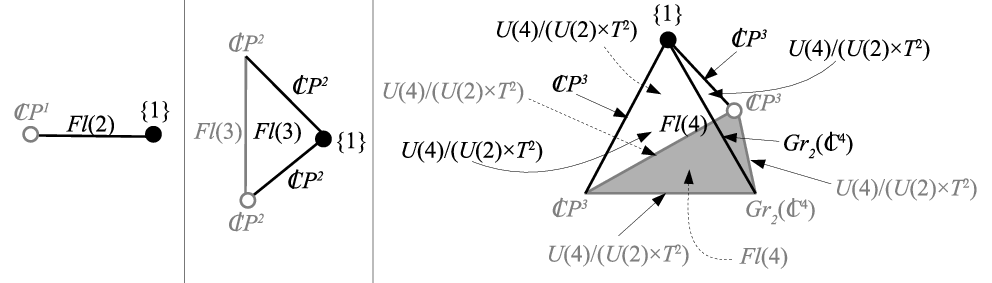
where U​(ℋ𝒮)σ={U∈U⁡(ℋ𝒮),U​σ​U−1=σ}U({\mathcal{H}_{\mathcal{S}}})_{\sigma}=\{U\in U({\mathcal{H}_{\mathcal{S}}}),U\sigma U^{-1}=\sigma\} is the isotropy subgroup (the stabilizer) of σ\sigma. The bundle 𝒟0​(ℋ𝒮)→πDΣ⁡(ℋ𝒮)\mathcal{D}_{0}({\mathcal{H}_{\mathcal{S}}})\xrightarrow{\pi_{D}}\Sigma({\mathcal{H}_{\mathcal{S}}}) is not locally trivial, it is a stratified space[3, 32]. A stratum Σi​(ℋ𝒮)\Sigma^{i}({\mathcal{H}_{\mathcal{S}}}) of Σ⁡(ℋ𝒮)\Sigma({\mathcal{H}_{\mathcal{S}}}) is characterized by the degeneracy profil of the eigenvalues. If σ∈Σi​(ℋ𝒮)\sigma\in\Sigma^{i}({\mathcal{H}_{\mathcal{S}}}) has k1k_{1} eigenvalues with degeneracy equal to q1q_{1}, k2k_{2} eigenvalues with degeneracy equal to q2q_{2}, etc, then its stabilizer is U​(ℋ𝒮)σ≃U​(q1)k1×…×U​(ql)klU({\mathcal{H}_{\mathcal{S}}})_{\sigma}\simeq U(q_{1})^{k_{1}}\times...\times U(q_{l})^{k_{l}} (the products are the group direct products) and then πD−1​(σ)≃U⁡(n)/(U​(q1)k1×…×U​(ql)kl)\pi_{D}^{-1}(\sigma)\simeq U(n)/(U(q_{1})^{k_{1}}\times...\times U(q_{l})^{k_{l}}) (∑iki​qi=n\sum_{i}k_{i}q_{i}=n). The stratum Σ∘​(ℋ𝒮)\Sigma^{\circ}({\mathcal{H}_{\mathcal{S}}}) with no eigenvalue degeneracy is associated with the normalizer U​(ℋ𝒮)σ≃TnU({\mathcal{H}_{\mathcal{S}}})_{\sigma}\simeq T^{n} (the nn-torus) and ∀σ∈Σ∘​(ℋ𝒮)\forall\sigma\in\Sigma^{\circ}({\mathcal{H}_{\mathcal{S}}}), πD−1​(σ)≃U⁡(n)/Tn=F​l​(n,ℂ)\pi_{D}^{-1}(\sigma)\simeq U(n)/T^{n}=Fl(n,\mathbb{C}) (the flag manifold); in the other cases, the fibers of the strata in D0​(ℋ𝒮)D_{0}({\mathcal{H}_{\mathcal{S}}}) are homeomorphic to partial flag manifolds as Grassmanian manifolds G​rp​(ℂn)=U⁡(n)/(U⁡(n−p)×U⁡(p))Gr_{p}(\mathbb{C}^{n})=U(n)/(U(n-p)\times U(p)), projective manifolds ℂ​Pn−1=U⁡(n)/(U⁡(n−1)×U⁡(1))\mathbb{C}P^{n-1}=U(n)/(U(n-1)\times U(1)), etc. We distinguish between the regular strata such that detρ≠0\det\rho\not=0 (no zero eigenvalue) and the singular strata such that detρ=0\det\rho=0. We remark the presence of two particular strata associated with vertices of Σ⁡(n)\Sigma(n), the singular stratum of the pure states Σ0​(ℋ𝒮)\Sigma^{0}({\mathcal{H}_{\mathcal{S}}}) (p1=…=pn−1=0p_{1}=...=p_{n-1}=0 and pn=1p_{n}=1, πD−1​(σ)≃U⁡(n)/(U⁡(n−1)×U⁡(1))=ℂ​Pn−1\pi_{D}^{-1}(\sigma)\simeq U(n)/(U(n-1)\times U(1))=\mathbb{C}P^{n-1}), and the regular stratum of the microcanonical state Σ∞​(ℋ𝒮)\Sigma^{\infty}({\mathcal{H}_{\mathcal{S}}}) (p1=…=pn=1np_{1}=...=p_{n}=\frac{1}{n}, πD−1​(σ)≃U⁡(n)/U⁡(n)={1}\pi_{D}^{-1}(\sigma)\simeq U(n)/U(n)=\{1\}). Fig. 1 illustrates the stratification for the smallest dimensional cases.
Refer to caption
Figure 1: The simplex Σ⁡(n)\Sigma(n) for n=2n=2 (left), n=3n=3 (middle) and n=4n=4 (right). The strata are the open sub-simplices of each simplex (including Σ∘​(n)\Sigma^{\circ}(n) the interior of Σ⁡(n)\Sigma(n) – the stratum with no degenerated eigenvalues –). For each stratum Σi\Sigma^{i} the model manifold of πD−1​(σ)\pi^{-1}_{D}(\sigma) is indicated. Singular strata are written in grey whereas regular strata are written in black (∙\bullet denotes the stratum of the microcanonical state, and ∘\circ denotes the stratum of the pure states). The description of the simplexes can be found table 1. The details about the stratification can found in ref.[3] where Σ⁡(n)\Sigma(n) is called Weyl chamber by analogy with the group representation theory.
Table 1: Descriptions of the stratification of the simplex Σ⁡(n)\Sigma(n).
nn strata Σi​(n)\Sigma^{i}(n) sub-simplices fiber πD−1​(σ)\pi_{D}^{-1}(\sigma)
2 0<p1<p20<p_{1}<p_{2} edge F​l​(2,ℂ)Fl(2,\mathbb{C})
p1=p2=1/2p_{1}=p_{2}=1/2 vertex {1}\{1\}
p1=0<p2=1p_{1}=0<p_{2}=1 vertex ℂ​P1\mathbb{C}P^{1}
3 0<p1<p2<p30<p_{1}<p_{2}<p_{3} facet F​l​(3,ℂ)Fl(3,\mathbb{C})
0<p1=p2<p30<p_{1}=p_{2}<p_{3} edges ℂ​P2\mathbb{C}P^{2}
0<p1<p2=p30<p_{1}<p_{2}=p_{3}
p1=0<p2<p3p_{1}=0<p_{2}<p_{3} edge F​l​(3,ℂ)Fl(3,\mathbb{C})
p1=0<p2=p3=1/2p_{1}=0<p_{2}=p_{3}=1/2 vertices ℂ​P2\mathbb{C}P^{2}
p1=p2=0<p3=1p_{1}=p_{2}=0<p_{3}=1
p1=p2=p3=1/3p_{1}=p_{2}=p_{3}=1/3 vertex {1}\{1\}
4 0<p1<p2<p3<p40<p_{1}<p_{2}<p_{3}<p_{4} cell F​l​(4,ℂ)Fl(4,\mathbb{C})
0<p1=p2<p3<p40<p_{1}=p_{2}<p_{3}<p_{4} facets U⁡(4)/(U⁡(2)×T2)U(4)/(U(2)\times T^{2})
0<p1<p2=p3<p40<p_{1}<p_{2}=p_{3}<p_{4}
0<p1<p2<p3=p40<p_{1}<p_{2}<p_{3}=p_{4}
0=p1<p2<p3<p40=p_{1}<p_{2}<p_{3}<p_{4} facet F​l​(4,ℂ)Fl(4,\mathbb{C})
0<p1=p2<p3=p40<p_{1}=p_{2}<p_{3}=p_{4} edge G​r2​(ℂ4)Gr_{2}(\mathbb{C}^{4})
0<p1=p2=p3<p40<p_{1}=p_{2}=p_{3}<p_{4} edges ℂ​P3\mathbb{C}P^{3}
0<p1<p2=p3=p40<p_{1}<p_{2}=p_{3}=p_{4}
p1=0<p2<p3=p4p_{1}=0<p_{2}<p_{3}=p_{4} edges U⁡(4)/(U⁡(2)×T2)U(4)/(U(2)\times T^{2})
p1=0<p2=p3<p4p_{1}=0<p_{2}=p_{3}<p_{4}
p1=p2=0<p3<p4p_{1}=p_{2}=0<p_{3}<p_{4}
p1=p2=p3=0<p4=1p_{1}=p_{2}=p_{3}=0<p_{4}=1 vertices ℂ​P3\mathbb{C}P^{3}
p1=0<p2=p3=p4=1/3p_{1}=0<p_{2}=p_{3}=p_{4}=1/3
p1=p2=0<p3=p4=1/2p_{1}=p_{2}=0<p_{3}=p_{4}=1/2 vertex G​r2​(ℂ4)Gr_{2}(\mathbb{C}^{4})
p1=p2=p3=p4=1/4p_{1}=p_{2}=p_{3}=p_{4}=1/4 vertex {1}\{1\}

Let ℋ𝒜{\mathcal{H}_{\mathcal{A}}} be an arbitrary ancilla, and let (ζi)i=1,…,n(\zeta_{i})_{i=1,...,n} and (ξα)α=1,…,n(\xi_{\alpha})_{\alpha=1,...,n} be orthonormal basis of ℋ𝒮{\mathcal{H}_{\mathcal{S}}} and ℋ𝒜{\mathcal{H}_{\mathcal{A}}}. Let 𝚿:ℬ⁡(ℋ𝒮)→≃ℋ𝒮⊗ℋ𝒜\mathbf{\Psi}:\mathcal{B}({\mathcal{H}_{\mathcal{S}}})\xrightarrow{\simeq}{\mathcal{H}_{\mathcal{S}}}\otimes{\mathcal{H}_{\mathcal{A}}} be the (non canonical) isomorphism defined by

∀W∈ℬ⁡(ℋ𝒮),𝚿⁡(W)=Wi​α​ζi⊗ξα\forall W\in\mathcal{B}({\mathcal{H}_{\mathcal{S}}}),\quad\mathbf{\Psi}(W)=W^{i\alpha}\zeta_{i}\otimes\xi_{\alpha} (12)

with W=Wi​α​|ζi⟩​⟨ζα|W=W^{i\alpha}|\zeta_{i}\rangle\langle\zeta_{\alpha}|. The restriction of 𝚿\mathbf{\Psi} on SH​S​ℬ​(ℋ𝒮)S_{HS}\mathcal{B}({\mathcal{H}_{\mathcal{S}}}) has its values in S⁡(ℋ𝒮⊗ℋ𝒜)={Ψ∈ℋ𝒮⊗ℋ𝒜,‖Ψ‖ℋ𝒮⊗ℋ𝒜=1}≃S2​n2−1S({\mathcal{H}_{\mathcal{S}}}\otimes{\mathcal{H}_{\mathcal{A}}})=\{\Psi\in{\mathcal{H}_{\mathcal{S}}}\otimes{\mathcal{H}_{\mathcal{A}}},\|\Psi\|_{{\mathcal{H}_{\mathcal{S}}}\otimes{\mathcal{H}_{\mathcal{A}}}}=1\}\simeq S^{2n^{2}-1} (the (2​n2−1)(2n^{2}-1)-dimensional sphere). Note that ⟨⟨𝚿⁡(Z)|𝚿⁡(W)⟩⟩=⟨Z|W⟩H​S\langle\hskip-1.99997pt\langle\mathbf{\Psi}(Z)|\mathbf{\Psi}(W)\rangle\hskip-1.99997pt\rangle=\langle Z|W\rangle_{HS}.
The following commutative diagramm summarizes the bundle of purification:

SH​S​ℬ​(ℋ𝒮)→Ψ≃S⁡(ℋ𝒮⊗ℋ𝒜)→≃S2​n2−1πH​S↓π𝒜↓↓𝒟0​(ℋ𝒮)=𝒟0​(ℋ𝒮)→≃𝒟0​(ℂn)=⨆i𝒟0i​(ℂn)←↩U⁡(n)/U​(n)σπD↓πD↓↓↓↓Σ⁡(ℋ𝒮)=Σ⁡(ℋ𝒮)→≃Σ⁡(n)=⨆iΣi​(n)←↩{σ}\begin{CD}S_{HS}\mathcal{B}({\mathcal{H}_{\mathcal{S}}})@>{\simeq}>{\Psi}>S({\mathcal{H}_{\mathcal{S}}}\otimes{\mathcal{H}_{\mathcal{A}}})@>{\simeq}>{}>S^{2n^{2}-1}\\ @V{\pi_{HS}}V{}V@V{\pi_{\mathcal{A}}}V{}V@V{}V{}V\\ \mathcal{D}_{0}({\mathcal{H}_{\mathcal{S}}})=\mathcal{D}_{0}({\mathcal{H}_{\mathcal{S}}})@>{\simeq}>{}>\mathcal{D}_{0}(\mathbb{C}^{n})=\bigsqcup_{i}\mathcal{D}^{i}_{0}(\mathbb{C}^{n})@<{\hookleftarrow}<{}<U(n)/U(n)_{\sigma}\\ @V{\pi_{D}}V{}V@V{\pi_{D}}V{}V@V{}V{}V@V{}V{}V@V{}V{}V\\ \Sigma({\mathcal{H}_{\mathcal{S}}})=\Sigma({\mathcal{H}_{\mathcal{S}}})@>{\simeq}>{}>\Sigma(n)=\bigsqcup_{i}\Sigma^{i}(n)@<{\hookleftarrow}<{}<\{\sigma\}\end{CD}

where ↩\hookleftarrow denotes inclusion maps and ≃\simeq denotes homeomorphisms, the vertical arrows are projections.
The ancilla plays the role of an effective environment with which the system is entangled. The right action of U⁡(ℋ𝒮)U({\mathcal{H}_{\mathcal{S}}}) on SH​S​ℬ​(ℋ𝒮)S_{HS}\mathcal{B}({\mathcal{H}_{\mathcal{S}}}) is associated with unitary transformations of ℋ𝒜{\mathcal{H}_{\mathcal{A}}}.

∀U∈U⁡(ℋ𝒮),∀W∈SH​S​ℬ​(ℋ𝒮),𝚿⁡(W​U)=1ℋ𝒮⊗Ut​𝚿​(W)⇒πΨ​(𝚿⁡(W​U))=ρW\forall U\in U({\mathcal{H}_{\mathcal{S}}}),\forall W\in S_{HS}\mathcal{B}({\mathcal{H}_{\mathcal{S}}}),\quad\mathbf{\Psi}(WU)=1_{\mathcal{H}_{\mathcal{S}}}\otimes U^{\text{{t}}}\mathbf{\Psi}(W)\Rightarrow\pi_{\Psi}(\mathbf{\Psi}(WU))=\rho_{W} (13)

where Ut=⟨ζβ​|U​ζα⟩|ξα⟩​⟨ξβ|∈U⁡(ℋ𝒜)U^{\text{{t}}}=\langle\zeta_{\beta}|U\zeta^{\alpha}\rangle|\xi_{\alpha}\rangle\langle\xi^{\beta}|\in U({\mathcal{H}_{\mathcal{A}}}) (t denotes the transposition) and ρW=π𝒜​(𝚿⁡(W))=πH​S​(W)=W​W†\rho_{W}=\pi_{\mathcal{A}}(\mathbf{\Psi}(W))=\pi_{HS}(W)=WW^{\dagger}. Such a transformation has no consequence for the observator which has only information concerning the system (information concerning the environment is lost by the partial trace trℋ𝒜\mathrm{tr}_{\mathcal{H}_{\mathcal{A}}}). It is then associated with an inobservable reconfiguration of the ancilla (the effective environment). In contrast, the left action of U⁡(ℋ𝒮)U({\mathcal{H}_{\mathcal{S}}}) on SH​S​ℬ​(ℋ𝒮)S_{HS}\mathcal{B}({\mathcal{H}_{\mathcal{S}}}) is associated with unitary transformations of ℋ𝒮{\mathcal{H}_{\mathcal{S}}} modifying the mixed state:

∀U∈U⁡(ℋ𝒮),∀W∈SH​S​ℬ​(ℋ𝒮),𝚿⁡(U​W)=U⊗1ℋ𝒜​Ψ​(W)⇒πΨ​(𝚿⁡(U​W))=U​ρW​U−1\forall U\in U({\mathcal{H}_{\mathcal{S}}}),\forall W\in S_{HS}\mathcal{B}({\mathcal{H}_{\mathcal{S}}}),\quad\mathbf{\Psi}(UW)=U\otimes 1_{\mathcal{H}_{\mathcal{A}}}\Psi(W)\Rightarrow\pi_{\Psi}(\mathbf{\Psi}(UW))=U\rho_{W}U^{-1} (14)

In quantum information, it can be interesting to consider also SLOCC transformations (Stochastic Local Operations and Classical Communication). By virtue of the principle of the quantum open systems, information concerning the ancilla (the environment) is lost by taking the partial trace (information stored in the environment is not directly accessible), the physicist cannot performs SLOCC transformations on ℋ𝒜{\mathcal{H}_{\mathcal{A}}}. The group of SLOCC transformations on ℋ𝒮{\mathcal{H}_{\mathcal{S}}} is S​L​(ℋ𝒮)≃S​L​(n,ℂ)SL({\mathcal{H}_{\mathcal{S}}})\simeq SL(n,\mathbb{C}) (the group of invertible operators of ℋ𝒮{\mathcal{H}_{\mathcal{S}}} with determinant equal to 1). Since U⁡(ℋ𝒮)⊃S​U​(ℋ𝒮)⊂S​L​(ℋ𝒮)U({\mathcal{H}_{\mathcal{S}}})\supset SU({\mathcal{H}_{\mathcal{S}}})\subset SL({\mathcal{H}_{\mathcal{S}}}) (S​U​(ℋ𝒮)SU({\mathcal{H}_{\mathcal{S}}}) is the group of unitary operators of ℋ𝒮{\mathcal{H}_{\mathcal{S}}} with determinant equal to 1), the group of unitary and SLOCC transformations are S​L​(ℋ𝒮)×U⁡(1)=G​L​(ℋ𝒮)SL({\mathcal{H}_{\mathcal{S}}})\times U(1)=GL({\mathcal{H}_{\mathcal{S}}}) (U⁡(1)U(1) is the group of phase changes and G​L​(ℋ𝒮)GL({\mathcal{H}_{\mathcal{S}}}) is the group of invertible operators of ℋ𝒮{\mathcal{H}_{\mathcal{S}}}).

∀U∈G​L​(ℋ𝒮),∀W∈ℬ⁡(ℋ𝒮),𝚿⁡(U​W)=U⊗1ℋ𝒜​𝚿​(W)⇒πΨ​(𝚿⁡(U​W))=U​ρW​U†\forall U\in GL({\mathcal{H}_{\mathcal{S}}}),\forall W\in\mathcal{B}({\mathcal{H}_{\mathcal{S}}}),\quad\mathbf{\Psi}(UW)=U\otimes 1_{\mathcal{H}_{\mathcal{A}}}\mathbf{\Psi}(W)\Rightarrow\pi_{\Psi}(\mathbf{\Psi}(UW))=U\rho_{W}U^{\dagger} (15)

by noting that SH​S​ℬ​(ℋ𝒮)S_{HS}\mathcal{B}({\mathcal{H}_{\mathcal{S}}}) and 𝒟0​(ℋ𝒮)\mathcal{D}_{0}({\mathcal{H}_{\mathcal{S}}}) are not stable by the right action of S​L​(ℋ𝒮)SL({\mathcal{H}_{\mathcal{S}}}) (we must then consider ℬ⁡(ℋ𝒮)\mathcal{B}({\mathcal{H}_{\mathcal{S}}}) and 𝒟⁡(ℋ𝒮)\mathcal{D}({\mathcal{H}_{\mathcal{S}}})). We extend πD\pi_{D} on the whole of 𝒟⁡(ℋ𝒮)\mathcal{D}({\mathcal{H}_{\mathcal{S}}}) by ∀U∈S​L​(ℋ𝒮)\forall U\in SL({\mathcal{H}_{\mathcal{S}}}), ∀ρ∈𝒟0​(ℋ𝒮)\forall\rho\in\mathcal{D}_{0}({\mathcal{H}_{\mathcal{S}}}), πD​(U​ρ​U†)=πD​(ρ)\pi_{D}(U\rho U^{\dagger})=\pi_{D}(\rho).

2.2 The C∗C^{*}-module structure

The purification space ℋ𝒮⊗ℋ𝒜{\mathcal{H}_{\mathcal{S}}}\otimes{\mathcal{H}_{\mathcal{A}}} can also be viewed as a left Hilbert ℬ⁡(ℋ𝒮)\mathcal{B}({\mathcal{H}_{\mathcal{S}}})-C∗C^{*}-module[33], the left action of the C∗C^{*}-algebra ℬ⁡(ℋ𝒮)\mathcal{B}({\mathcal{H}_{\mathcal{S}}}) being defined by

∀A∈ℬ⁡(ℋ𝒮),∀Ψ∈ℋ𝒮⊗ℋ𝒜,A​Ψ=A⊗1ℋ𝒜​Ψ=Ψi​α​(A​ζi)⊗ξα\forall A\in\mathcal{B}({\mathcal{H}_{\mathcal{S}}}),\forall\Psi\in{\mathcal{H}_{\mathcal{S}}}\otimes{\mathcal{H}_{\mathcal{A}}},\quad A\Psi=A\otimes 1_{\mathcal{H}_{\mathcal{A}}}\Psi=\Psi^{i\alpha}(A\zeta_{i})\otimes\xi_{\alpha} (16)

The inner product of the C∗C^{*}-module is defined by

∀Ψ,Φ∈ℋ𝒮⊗ℋ𝒜,⟨Φ|Ψ⟩∗=trℋ𝒜|Ψ⟩⟩⟨⟨Φ|∈ℬ(ℋ𝒮)\forall\Psi,\Phi\in{\mathcal{H}_{\mathcal{S}}}\otimes{\mathcal{H}_{\mathcal{A}}},\quad\langle\Phi|\Psi\rangle_{*}=\mathrm{tr}_{\mathcal{H}_{\mathcal{A}}}|\Psi\rangle\hskip-1.99997pt\rangle\langle\hskip-1.99997pt\langle\Phi|\in\mathcal{B}({\mathcal{H}_{\mathcal{S}}}) (17)

It satisfies the usual properties:

∀A,B∈ℬ⁡(ℋ𝒮),∀Ψ,Φ,Ξ∈ℋ𝒮⊗ℋ𝒜,⟨Φ|A​Ψ+B​Ξ⟩∗=A​⟨Φ|Ψ⟩∗+B​⟨Φ|Ξ⟩∗\forall A,B\in\mathcal{B}({\mathcal{H}_{\mathcal{S}}}),\forall\Psi,\Phi,\Xi\in{\mathcal{H}_{\mathcal{S}}}\otimes{\mathcal{H}_{\mathcal{A}}},\quad\langle\Phi|A\Psi+B\Xi\rangle_{*}=A\langle\Phi|\Psi\rangle_{*}+B\langle\Phi|\Xi\rangle_{*} (18)
∀Ψ,Φ∈ℋ𝒮⊗ℋ𝒜,⟨Φ|Ψ⟩∗†=⟨Ψ|Φ⟩∗\forall\Psi,\Phi\in{\mathcal{H}_{\mathcal{S}}}\otimes{\mathcal{H}_{\mathcal{A}}},\quad\langle\Phi|\Psi\rangle^{\dagger}_{*}=\langle\Psi|\Phi\rangle_{*} (19)
∀Ψ∈ℋ𝒮⊗ℋ𝒜,⟨Ψ|Ψ⟩∗≥0​ and ​⟨Ψ|Ψ⟩∗=0⇔Ψ=0\forall\Psi\in{\mathcal{H}_{\mathcal{S}}}\otimes{\mathcal{H}_{\mathcal{A}}},\quad\langle\Psi|\Psi\rangle_{*}\geq 0\text{ and }\langle\Psi|\Psi\rangle_{*}=0\iff\Psi=0 (20)

The density operator associated with a state of ℋ𝒮⊗ℋ𝒜{\mathcal{H}_{\mathcal{S}}}\otimes{\mathcal{H}_{\mathcal{A}}} is its square norm with respect to the C∗C^{*}-module structure:

∀Ψ∈ℋ𝒮⊗ℋ𝒜,‖Ψ‖∗2=⟨Ψ|Ψ⟩∗=ρΨ∈𝒟⁡(ℋ𝒮)\forall\Psi\in{\mathcal{H}_{\mathcal{S}}}\otimes{\mathcal{H}_{\mathcal{A}}},\quad\|\Psi\|^{2}_{*}=\langle\Psi|\Psi\rangle_{*}=\rho_{\Psi}\in\mathcal{D}({\mathcal{H}_{\mathcal{S}}}) (21)

ℬ⁡(ℋ𝒮)\mathcal{B}({\mathcal{H}_{\mathcal{S}}}) as the standard purification space is related to the C∗C^{*}-module structure by

∀A∈ℬ⁡(ℋ𝒮),∀W∈ℬ⁡(ℋ𝒮),𝚿⁡(A​W)=A​𝚿​(W)\forall A\in\mathcal{B}({\mathcal{H}_{\mathcal{S}}}),\forall W\in\mathcal{B}({\mathcal{H}_{\mathcal{S}}}),\quad\mathbf{\Psi}(AW)=A\mathbf{\Psi}(W) (22)
∀W,Z∈ℬ⁡(ℋ𝒮),⟨𝚿⁡(W)|𝚿⁡(Z)⟩∗=Z​W†\forall W,Z\in\mathcal{B}({\mathcal{H}_{\mathcal{S}}}),\quad\langle\mathbf{\Psi}(W)|\mathbf{\Psi}(Z)\rangle_{*}=ZW^{\dagger} (23)

The right action of ℬ⁡(ℋ𝒮)\mathcal{B}({\mathcal{H}_{\mathcal{S}}}) on itself induces a particular class of operators of the C∗C^{*}-module acting only on ℋ𝒜{\mathcal{H}_{\mathcal{A}}}:

∀A∈ℬ⁡(ℋ𝒮),∀W∈ℬ⁡(ℋ𝒮),𝚿⁡(W​A)=1ℋ𝒮⊗At​𝚿​(W)\forall A\in\mathcal{B}({\mathcal{H}_{\mathcal{S}}}),\forall W\in\mathcal{B}({\mathcal{H}_{\mathcal{S}}}),\quad\mathbf{\Psi}(WA)=1_{\mathcal{H}_{\mathcal{S}}}\otimes A^{\text{{t}}}\mathbf{\Psi}(W) (24)

2.3 C∗C^{*}-adjointness

In this part we want to define the adjoint, with respect to the inner product of the C∗C^{*}-module, of the right action of ℬ⁡(ℋ𝒮)\mathcal{B}({\mathcal{H}_{\mathcal{S}}}) on ℋ𝒮⊗ℋ𝒜{\mathcal{H}_{\mathcal{S}}}\otimes{\mathcal{H}_{\mathcal{A}}}.

Definition 1

Let Γ∈ℬ⁡(ℋ𝒮)\Gamma\in\mathcal{B}({\mathcal{H}_{\mathcal{S}}}). We define Γ†:ℋ𝒮⊗ℋ𝒜→ℬ⁡(ℋ𝒮)\Gamma^{\rotatebox{180.0}{\scriptsize$\dagger$}}:{\mathcal{H}_{\mathcal{S}}}\otimes{\mathcal{H}_{\mathcal{A}}}\to\mathcal{B}({\mathcal{H}_{\mathcal{S}}}) by

∀Ψ∈ℋ𝒮⊗ℋ𝒜,Γ†​(Ψ)\displaystyle\forall\Psi\in{\mathcal{H}_{\mathcal{S}}}\otimes{\mathcal{H}_{\mathcal{A}}},\quad\Gamma^{\rotatebox{180.0}{\scriptsize$\dagger$}}(\Psi) =\displaystyle= Γij​Ψj​α​(WΨ⋆)β​i​|ξα⟩​⟨ξβ|\displaystyle{\Gamma^{i}}_{j}\Psi^{j\alpha}(W^{\star}_{\Psi})_{\beta i}|\xi_{\alpha}\rangle\langle\xi^{\beta}| (25)
=\displaystyle= (WΨ⋆​Γ​WΨ)βα​|ξα⟩​⟨ξβ|\displaystyle{(W^{\star}_{\Psi}\Gamma W_{\Psi})_{\beta}}^{\alpha}|\xi_{\alpha}\rangle\langle\xi^{\beta}| (26)
=\displaystyle= (WΨ⋆​Γ​WΨ)tαβ​|ξα⟩​⟨ξβ|\displaystyle{{(W^{\star}_{\Psi}\Gamma W_{\Psi})^{\text{{t}}}}^{\alpha}}_{\beta}|\xi_{\alpha}\rangle\langle\xi^{\beta}| (27)

where WΨ∈ℬ⁡(ℋ𝒮)W_{\Psi}\in\mathcal{B}({\mathcal{H}_{\mathcal{S}}}) is such that 𝚿⁡(WΨ)=Ψ\mathbf{\Psi}(W_{\Psi})=\Psi, Γij=⟨ζi|Γ​ζj⟩{\Gamma^{i}}_{j}=\langle\zeta^{i}|\Gamma\zeta_{j}\rangle, Ψj​α=WΨj​α=⟨ζj|WΨ​ζα⟩=⟨⟨ζj⊗ξα|Ψ⟩⟩\Psi^{j\alpha}=W^{j\alpha}_{\Psi}=\langle\zeta^{j}|W_{\Psi}\zeta^{\alpha}\rangle=\langle\hskip-1.99997pt\langle\zeta^{j}\otimes\xi^{\alpha}|\Psi\rangle\hskip-1.99997pt\rangle, and where WΨ⋆∈ℬ⁡(ℋ𝒮)W^{\star}_{\Psi}\in\mathcal{B}({\mathcal{H}_{\mathcal{S}}}) is the pseudo-inverse of WΨW_{\Psi}:

WΨ⋆​WΨ=1−Pker⁡WΨ​ and ​WΨ​WΨ⋆=PRan​WΨW^{\star}_{\Psi}W_{\Psi}=1-P_{\ker W_{\Psi}}\text{ and }W_{\Psi}W^{\star}_{\Psi}=P_{\mathrm{Ran}W_{\Psi}} (28)

where Pker⁡WΨP_{\ker W_{\Psi}} and PRan​WΨP_{\mathrm{Ran}W_{\Psi}} are respectively the projections on the kernel and on the range of WΨW_{\Psi} in ℋ𝒮{\mathcal{H}_{\mathcal{S}}}.

Property 1

Let Γ‡​(Ψ)=Γ†​(Ψ)†\Gamma^{\ddagger}(\Psi)=\Gamma^{\rotatebox{180.0}{\scriptsize$\dagger$}}(\Psi)^{\dagger} (the adjoint †\dagger is in the sense of the inner product of ℋ𝒜{\mathcal{H}_{\mathcal{A}}}). We have

∀Φ∈ℋ𝒮⊗ℋ𝒜,\displaystyle\forall\Phi\in{\mathcal{H}_{\mathcal{S}}}\otimes{\mathcal{H}_{\mathcal{A}}}, ⟨Φ|1ℋ𝒮⊗Γ†​(Ψ)​Ψ⟩∗=⟨1ℋ𝒮⊗Γ‡​(Ψ)​Φ|Ψ⟩∗\displaystyle\langle\Phi|1_{\mathcal{H}_{\mathcal{S}}}\otimes\Gamma^{\rotatebox{180.0}{\scriptsize$\dagger$}}(\Psi)\Psi\rangle_{*}=\langle 1_{\mathcal{H}_{\mathcal{S}}}\otimes\Gamma^{\ddagger}(\Psi)\Phi|\Psi\rangle_{*} (29)
⇔\displaystyle\iff ⟨Φ|PRan​WΨ​Γ⊗1ℋ𝒜​Ψ⟩∗=⟨1ℋ𝒮⊗Γ‡​(Ψ)​Φ|Ψ⟩∗\displaystyle\langle\Phi|P_{\mathrm{Ran}W_{\Psi}}\Gamma\otimes 1_{\mathcal{H}_{\mathcal{A}}}\Psi\rangle_{*}=\langle 1_{\mathcal{H}_{\mathcal{S}}}\otimes\Gamma^{\ddagger}(\Psi)\Phi|\Psi\rangle_{*} (30)

For this reason, we call Γ‡\Gamma^{\ddagger} the C∗C^{*}-adjoint of Γ\Gamma.

Corollary 1
∀Ψ∈ℋ𝒮⊗ℋ𝒜,1ℋ𝒮⊗Γ†​(Ψ)​Ψ=PRan​WΨ​Γ⊗1ℋ𝒜​Ψ\forall\Psi\in{\mathcal{H}_{\mathcal{S}}}\otimes{\mathcal{H}_{\mathcal{A}}},\quad 1_{\mathcal{H}_{\mathcal{S}}}\otimes\Gamma^{\rotatebox{180.0}{\scriptsize$\dagger$}}(\Psi)\Psi=P_{\mathrm{Ran}W_{\Psi}}\Gamma\otimes 1_{\mathcal{H}_{\mathcal{A}}}\Psi (31)

Proof:

1ℋ𝒮⊗Γ†​(Ψ)​Ψ\displaystyle 1_{\mathcal{H}_{\mathcal{S}}}\otimes\Gamma^{\rotatebox{180.0}{\scriptsize$\dagger$}}(\Psi)\Psi =\displaystyle= Γ†​(Ψ)αβ​Ψi​β​ζi⊗ξα\displaystyle{\Gamma^{\rotatebox{180.0}{\scriptsize$\dagger$}}(\Psi)^{\alpha}}_{\beta}\Psi^{i\beta}\zeta_{i}\otimes\xi_{\alpha} (32)
=\displaystyle= Γkj​Ψj​α​(WΨ⋆)β​k​Ψi​β​ζi⊗ξα\displaystyle{\Gamma^{k}}_{j}\Psi^{j\alpha}(W_{\Psi}^{\star})_{\beta k}\Psi^{i\beta}\zeta_{i}\otimes\xi_{\alpha} (33)
=\displaystyle= Γkj​Ψj​α​(WΨ​WΨ⋆)ik​ζi⊗ξα\displaystyle{\Gamma^{k}}_{j}\Psi^{j\alpha}{(W_{\Psi}W_{\Psi}^{\star})^{i}}_{k}\zeta_{i}\otimes\xi_{\alpha} (34)
=\displaystyle= (PRan​WΨ)ik​Γkj​Ψj​α​ζi⊗ξα\displaystyle{(P_{\mathrm{Ran}W_{\Psi}})^{i}}_{k}{\Gamma^{k}}_{j}\Psi^{j\alpha}\zeta_{i}\otimes\xi_{\alpha} (35)
=\displaystyle= PRan​WΨ​Γ⊗1ℋ𝒮​Ψ\displaystyle P_{\mathrm{Ran}W_{\Psi}}\Gamma\otimes 1_{\mathcal{H}_{\mathcal{S}}}\Psi (36)
⟨Φ|1ℋ𝒮⊗Γ†​(Ψ)​Ψ⟩∗\displaystyle\langle\Phi|1_{\mathcal{H}_{\mathcal{S}}}\otimes\Gamma^{\rotatebox{180.0}{\scriptsize$\dagger$}}(\Psi)\Psi\rangle_{*} =\displaystyle= trℋ𝒜|1ℋ𝒮⊗Γ†(Ψ)Ψ⟩⟩⟨⟨Φ|\displaystyle\mathrm{tr}_{\mathcal{H}_{\mathcal{A}}}|1_{\mathcal{H}_{\mathcal{S}}}\otimes\Gamma^{\rotatebox{180.0}{\scriptsize$\dagger$}}(\Psi)\Psi\rangle\hskip-1.99997pt\rangle\langle\hskip-1.99997pt\langle\Phi| (37)
=\displaystyle= Γ†​(Ψ)αβ​Ψi​β​Φj​α¯​|ζi⟩​⟨ζj|\displaystyle{\Gamma^{\rotatebox{180.0}{\scriptsize$\dagger$}}(\Psi)^{\alpha}}_{\beta}\Psi^{i\beta}\overline{\Phi_{j\alpha}}|\zeta_{i}\rangle\langle\zeta^{j}| (38)
⟨1ℋ𝒮​Γ‡​(Ψ)​Φ|Ψ⟩∗\displaystyle\langle 1_{\mathcal{H}_{\mathcal{S}}}\Gamma^{\ddagger}(\Psi)\Phi|\Psi\rangle_{*} =\displaystyle= trℋ𝒜|Ψ⟩⟩⟨⟨1ℋ𝒮⊗Γ‡(Ψ)Φ|\displaystyle\mathrm{tr}_{\mathcal{H}_{\mathcal{A}}}|\Psi\rangle\hskip-1.99997pt\rangle\langle\hskip-1.99997pt\langle 1_{\mathcal{H}_{\mathcal{S}}}\otimes\Gamma^{\ddagger}(\Psi)\Phi| (39)
=\displaystyle= Ψi​β​Γ‡​(Ψ)βα¯​Φj​α¯​|ζi⟩​⟨ζj|\displaystyle\Psi^{i\beta}\overline{{\Gamma^{\ddagger}(\Psi)_{\beta}}^{\alpha}}\overline{\Phi_{j\alpha}}|\zeta_{i}\rangle\langle\zeta^{j}| (40)
=\displaystyle= Ψi​β​Γ†​(Ψ)αβ​Φj​α¯​|ζi⟩​⟨ζj|\displaystyle\Psi^{i\beta}{\Gamma^{\rotatebox{180.0}{\scriptsize$\dagger$}}(\Psi)^{\alpha}}_{\beta}\overline{\Phi_{j\alpha}}|\zeta_{i}\rangle\langle\zeta^{j}| (41)

□\Box
It can be interesting to relate Ran​WΨ\mathrm{Ran}W_{\Psi} (which appears in the definition of the C∗C^{*}-adjoint) with the density operator.

Property 2

Let Ψ∈ℋ𝒮⊗ℋ𝒜\Psi\in{\mathcal{H}_{\mathcal{S}}}\otimes{\mathcal{H}_{\mathcal{A}}}, WΨ∈ℬ⁡(ℋ𝒮)W_{\Psi}\in\mathcal{B}({\mathcal{H}_{\mathcal{S}}}) be such that 𝚿⁡(WΨ)=Ψ\mathbf{\Psi}(W_{\Psi})=\Psi, and ρΨ=‖Ψ‖∗2=π𝒜​(Ψ)=WΨ​WΨ†∈𝒟⁡(ℋ𝒮)\rho_{\Psi}=\|\Psi\|^{2}_{*}=\pi_{\mathcal{A}}(\Psi)=W_{\Psi}W_{\Psi}^{\dagger}\in\mathcal{D}({\mathcal{H}_{\mathcal{S}}}). We have Ran​WΨ=Ran​ρΨ\mathrm{Ran}W_{\Psi}=\mathrm{Ran}\rho_{\Psi} and coker​WΨ=ker⁡ρΨ\mathrm{coker}W_{\Psi}=\ker\rho_{\Psi}.

Proof: coker​Wψ={ϕ∈ℋ𝒮,Ψi​α​ϕ¯i=0}\mathrm{coker}W_{\psi}=\{\phi\in{\mathcal{H}_{\mathcal{S}}},\Psi^{i\alpha}\overline{\phi}_{i}=0\}. ϕ∈coker​WΨ⇒ϕ¯i​Ψi​α​Ψ¯j​α=0⇒ϕ¯i​(ρΨ)ij=0\phi\in\mathrm{coker}W_{\Psi}\Rightarrow\overline{\phi}_{i}\Psi^{i\alpha}\overline{\Psi}_{j\alpha}=0\Rightarrow\overline{\phi}_{i}{(\rho_{\Psi})^{i}}_{j}=0 since ρΨ=Ψi​α​Ψ¯j​α​|ζi⟩​⟨ζj|\rho_{\Psi}=\Psi^{i\alpha}\overline{\Psi}_{j\alpha}|\zeta_{i}\rangle\langle\zeta^{j}|. We have then ⟨ϕ|​ρΨ=0⇒ρΨ​|ϕ⟩=0⇒ϕ∈ker⁡ρΨ\langle\phi|\rho_{\Psi}=0\Rightarrow\rho_{\Psi}|\phi\rangle=0\Rightarrow\phi\in\ker\rho_{\Psi}. We have then coker​WΨ⊂ker⁡ρΨ\mathrm{coker}W_{\Psi}\subset\ker\rho_{\Psi}.
(ρΨ)ij​|ζi⟩=Ψi​α​Ψ¯j​α​|ζi⟩⇒∀ϕ∈ℋ𝒮,(ρΨ)ij​ϕj​|ζi⟩=Ψi​α​Ψ¯j​α​ϕj​|ζi⟩{(\rho_{\Psi})^{i}}_{j}|\zeta_{i}\rangle=\Psi^{i\alpha}\overline{\Psi}_{j\alpha}|\zeta_{i}\rangle\Rightarrow\forall\phi\in{\mathcal{H}_{\mathcal{S}}},{(\rho_{\Psi})^{i}}_{j}\phi^{j}|\zeta_{i}\rangle=\Psi^{i\alpha}\overline{\Psi}_{j\alpha}\phi^{j}|\zeta_{i}\rangle. We have then ∀ϕ∈ℋ𝒮,ρΨ​ϕ=WΨ​(WΨ†​ϕ)⇒ρΨ​ϕ∈Ran​WΨ\forall\phi\in{\mathcal{H}_{\mathcal{S}}},\rho_{\Psi}\phi=W_{\Psi}(W_{\Psi}^{\dagger}\phi)\Rightarrow\rho_{\Psi}\phi\in\mathrm{Ran}W_{\Psi}. We have then Ran​ρΨ⊂Ran​WΨ\mathrm{Ran}\rho_{\Psi}\subset\mathrm{Ran}W_{\Psi}.
Suppose that (ζi)i(\zeta_{i})_{i} the basis of ℋ𝒮{\mathcal{H}_{\mathcal{S}}} is the eigenbasis of ρΨ\rho_{\Psi}. (ρΨ)ij=Ψi​α​Ψ¯j​α=pi​δji{(\rho_{\Psi})^{i}}_{j}=\Psi^{i\alpha}\overline{\Psi}_{j\alpha}=p^{i}\delta^{i}_{j}. We can write ⟨Ψj|Ψi⟩ℋ𝒜=pi​δji\langle\Psi_{j}|\Psi^{i}\rangle_{\mathcal{H}_{\mathcal{A}}}=p^{i}\delta^{i}_{j} with Ψi=Ψi​α​ξα∈ℋ𝒜\Psi^{i}=\Psi^{i\alpha}\xi_{\alpha}\in{\mathcal{H}_{\mathcal{A}}}. We have then pi=‖Ψi‖ℋ𝒜2p^{i}=\|\Psi^{i}\|^{2}_{\mathcal{H}_{\mathcal{A}}}. It follows that pi=0⇒Ψi=0⇒Ψi​α=0,∀αp^{i}=0\Rightarrow\Psi^{i}=0\Rightarrow\Psi^{i\alpha}=0,\forall\alpha. Ran​WΨ={Ψi​α​ϕα​|ζi⟩,ϕα∈ℂ}\mathrm{Ran}W_{\Psi}=\{\Psi^{i\alpha}\phi_{\alpha}|\zeta_{i}\rangle,\phi_{\alpha}\in\mathbb{C}\} and then Ran​WΨ⊂coRan​ρΨ\mathrm{Ran}W_{\Psi}\subset\mathrm{coRan}\rho_{\Psi} (coRan​ρΨ=(ker⁡ρΨ)⊥\mathrm{coRan}\rho_{\Psi}=(\ker\rho_{\Psi})^{\bot}). But coRan​ρΨ=Ran​ρΨ†=Ran​ρΨ\mathrm{coRan}\rho_{\Psi}=\mathrm{Ran}\rho_{\Psi}^{\dagger}=\mathrm{Ran}\rho_{\Psi} (ρΨ†=ρΨ\rho_{\Psi}^{\dagger}=\rho_{\Psi}). We have then Ran​WΨ⊂Ran​ρΨ\mathrm{Ran}W_{\Psi}\subset\mathrm{Ran}\rho_{\Psi}.
The two last paragraphs show that Ran​WΨ=Ran​ρΨ\mathrm{Ran}W_{\Psi}=\mathrm{Ran}\rho_{\Psi}. The first one shows that coker​WΨ⊂ker⁡ρΨ\mathrm{coker}W_{\Psi}\subset\ker\rho_{\Psi} but dimcoker​WΨ=dimℋ𝒮−dimRan​WΨ\dim\mathrm{coker}W_{\Psi}=\dim{\mathcal{H}_{\mathcal{S}}}-\dim\mathrm{Ran}W_{\Psi} (by definition ℋ𝒮=Ran​WΨ​⊕⊥​coker​WΨ{\mathcal{H}_{\mathcal{S}}}=\mathrm{Ran}W_{\Psi}\overset{\bot}{\oplus}\mathrm{coker}W_{\Psi}). We have then dimcoker​WΨ=dimℋ𝒮−dimRan​ρΨ=dimker⁡ρΨ\dim\mathrm{coker}W_{\Psi}=\dim{\mathcal{H}_{\mathcal{S}}}-\dim\mathrm{Ran}\rho_{\Psi}=\dim\ker\rho_{\Psi} (by virtue of the rank-nullity theorem). This induces that coker​WΨ=ker⁡ρΨ\mathrm{coker}W_{\Psi}=\ker\rho_{\Psi}. □\Box

3 Purification of Lindblad dynamics

3.1 From the Lindblad equation to the nonlinear Schrödinger equation

Theorem 1

Let t↦ρ⁡(t)∈𝒟0​(ℋ𝒮)t\mapsto\rho(t)\in\mathcal{D}_{0}({\mathcal{H}_{\mathcal{S}}}) be a solution of the Lindblad equation

ı​ℏ​ρ˙=[H𝒮,ρ]−ı2​γk​{Γk†​Γk,ρ}+ı​γk​Γk​ρ​Γk†\imath\hbar\dot{\rho}=[H_{\mathcal{S}},\rho]-\frac{\imath}{2}\gamma^{k}\{\Gamma^{\dagger}_{k}\Gamma_{k},\rho\}+\imath\gamma^{k}\Gamma_{k}\rho\Gamma_{k}^{\dagger} (42)

with H𝒮∈ℬ⁡(ℋ𝒮)H_{\mathcal{S}}\in\mathcal{B}({\mathcal{H}_{\mathcal{S}}}) the system Hamiltonian, Γk∈ℬ⁡(ℋ𝒮)\Gamma_{k}\in\mathcal{B}({\mathcal{H}_{\mathcal{S}}}) the quantum jump operators and γk∈[0,1]\gamma^{k}\in[0,1] the relaxation rates. Let t↦Ψρ​(t)∈ℋ𝒮⊗ℋ𝒜t\mapsto\Psi_{\rho}(t)\in{\mathcal{H}_{\mathcal{S}}}\otimes{\mathcal{H}_{\mathcal{A}}} be a purification state of ρ⁡(t)\rho(t). Ψρ\Psi_{\rho} is solution of the following projected non-hermitian nonlinear Schrödinger equation:

(1ℋ𝒮⊗PRan​ρ)​ı​ℏ​Ψ˙ρ\displaystyle(1_{\mathcal{H}_{\mathcal{S}}}\otimes P_{\mathrm{Ran}\rho})\imath\hbar\dot{\Psi}_{\rho}
=(1ℋ𝒮⊗PRan​ρ)​(H𝒮⊗1ℋ𝒜​Ψρ−ı2​γk​Γk†​Γk⊗1ℋ𝒜​Ψρ+ı2​γk​Γk⊗Γk‡​(Ψρ)​Ψρ)\displaystyle=(1_{\mathcal{H}_{\mathcal{S}}}\otimes P_{\mathrm{Ran}\rho})\left(H_{\mathcal{S}}\otimes 1_{\mathcal{H}_{\mathcal{A}}}\Psi_{\rho}-\frac{\imath}{2}\gamma^{k}\Gamma^{\dagger}_{k}\Gamma_{k}\otimes 1_{\mathcal{H}_{\mathcal{A}}}\Psi_{\rho}+\frac{\imath}{2}\gamma^{k}\Gamma_{k}\otimes\Gamma_{k}^{\ddagger}(\Psi_{\rho})\Psi_{\rho}\right) (43)

Proof: Let Wρ​(t)∈ℬ⁡(ℋ𝒮)W_{\rho}(t)\in\mathcal{B}({\mathcal{H}_{\mathcal{S}}}) be a standard purification of ρ\rho, ρ=Wρ​Wρ†\rho=W_{\rho}W_{\rho}^{\dagger}, such that 𝚿⁡(Wρ)=Ψρ\mathbf{\Psi}(W_{\rho})=\Psi_{\rho}.

ı​ℏ​ρ˙=ℒ⁡(ρ)\displaystyle\imath\hbar\dot{\rho}=\mathcal{L}(\rho) (44)
⇒\displaystyle\Rightarrow ı​ℏ​W˙ρ​Wρ†+ı​ℏ​Wρ​W˙ρ†=[H𝒮,ρ]−ı2​γk​{Γk†​Γk,ρ}+2×ı2​γk​Γk​ρ​Γk†\displaystyle\imath\hbar\dot{W}_{\rho}W^{\dagger}_{\rho}+\imath\hbar W_{\rho}\dot{W}_{\rho}^{\dagger}=[H_{\mathcal{S}},\rho]-\frac{\imath}{2}\gamma^{k}\{\Gamma^{\dagger}_{k}\Gamma_{k},\rho\}+2\times\frac{\imath}{2}\gamma^{k}\Gamma_{k}\rho\Gamma_{k}^{\dagger} (46)
⇒\displaystyle\Rightarrow ı​ℏ​W˙ρ​Wρ†−(ı​ℏ​W˙ρ​Wρ†)†=H𝒮​ρ−ı2​γk​Γk†​Γk​ρ+ı2​γk​Γk​ρ​Γk†\displaystyle\imath\hbar\dot{W}_{\rho}W_{\rho}^{\dagger}-(\imath\hbar\dot{W}_{\rho}W_{\rho}^{\dagger})^{\dagger}=H_{\mathcal{S}}\rho-\frac{\imath}{2}\gamma^{k}\Gamma_{k}^{\dagger}\Gamma_{k}\rho+\frac{\imath}{2}\gamma^{k}\Gamma_{k}\rho\Gamma_{k}^{\dagger}
−(H𝒮​ρ−ı2​γk​Γk†​Γk​ρ+ı2​γk​Γk​ρ​Γk†)†\displaystyle\qquad-\left(H_{\mathcal{S}}\rho-\frac{\imath}{2}\gamma^{k}\Gamma_{k}^{\dagger}\Gamma_{k}\rho+\frac{\imath}{2}\gamma^{k}\Gamma_{k}\rho\Gamma_{k}^{\dagger}\right)^{\dagger}
⇒\displaystyle\Rightarrow ı​ℏ​W˙ρ​Wρ†=H𝒮​ρ−ı2​γk​Γk†​Γk​ρ+ı2​γk​Γk​ρ​Γk†+K\displaystyle\imath\hbar\dot{W}_{\rho}W_{\rho}^{\dagger}=H_{\mathcal{S}}\rho-\frac{\imath}{2}\gamma^{k}\Gamma_{k}^{\dagger}\Gamma_{k}\rho+\frac{\imath}{2}\gamma^{k}\Gamma_{k}\rho\Gamma_{k}^{\dagger}+K (47)

where K=K†K=K^{\dagger} is an arbitrary self-adjoint operator. We can set K=0K=0 without loss of generality.

ı​ℏ​W˙ρ​Wρ†=H𝒮​Wρ​Wρ†−ı2​γk​Γk†​Γk​Wρ​Wρ†+ı2​γk​Γk​Wρ​Wρ†​Γk†\displaystyle\imath\hbar\dot{W}_{\rho}W_{\rho}^{\dagger}=H_{\mathcal{S}}W_{\rho}W_{\rho}^{\dagger}-\frac{\imath}{2}\gamma^{k}\Gamma_{k}^{\dagger}\Gamma_{k}W_{\rho}W_{\rho}^{\dagger}+\frac{\imath}{2}\gamma^{k}\Gamma_{k}W_{\rho}W_{\rho}^{\dagger}\Gamma_{k}^{\dagger} (49)
⇒\displaystyle\Rightarrow ı​ℏ​W˙ρ​PcoRan​Wρ=H𝒮​Wρ​PcoRan​Wρ−ı2​γk​Γk†​Γk​Wρ​PcoRan​Wρ\displaystyle\imath\hbar\dot{W}_{\rho}P_{\mathrm{coRan}W_{\rho}}=H_{\mathcal{S}}W_{\rho}P_{\mathrm{coRan}W_{\rho}}-\frac{\imath}{2}\gamma^{k}\Gamma_{k}^{\dagger}\Gamma_{k}W_{\rho}P_{\mathrm{coRan}W_{\rho}}
+ı2​γk​Γk​Wρ​Wρ†​Γk†​(Wρ†)⋆\displaystyle\qquad+\frac{\imath}{2}\gamma^{k}\Gamma_{k}W_{\rho}W_{\rho}^{\dagger}\Gamma_{k}^{\dagger}(W_{\rho}^{\dagger})^{\star}

By application of 𝚿\mathbf{\Psi} on this last equation we find

1ℋ𝒮⊗PRan​ρ​ı​ℏ​Ψ˙ρ=H𝒮⊗PRan​ρ​Ψρ−ı2​γk​Γk†​Γk⊗PRan​ρ​Ψρ+ı2​γk​Γk⊗(Wρ†​Γk†​(Wρ†)⋆)t​Ψρ1_{\mathcal{H}_{\mathcal{S}}}\otimes P_{\mathrm{Ran}\rho}\imath\hbar\dot{\Psi}_{\rho}=H_{\mathcal{S}}\otimes P_{\mathrm{Ran}\rho}\Psi_{\rho}-\frac{\imath}{2}\gamma^{k}\Gamma^{\dagger}_{k}\Gamma_{k}\otimes P_{\mathrm{Ran}\rho}\Psi_{\rho}+\frac{\imath}{2}\gamma^{k}\Gamma_{k}\otimes(W_{\rho}^{\dagger}\Gamma_{k}^{\dagger}(W^{\dagger}_{\rho})^{\star})^{\text{{t}}}\Psi_{\rho} (50)

But (Wρ†​Γk†​(Wρ†)⋆)t=(Wρ⋆​Γk​Wρ)†t=Γk‡​(Ψρ)(W_{\rho}^{\dagger}\Gamma_{k}^{\dagger}(W^{\dagger}_{\rho})^{\star})^{\text{{t}}}=(W_{\rho}^{\star}\Gamma_{k}W_{\rho})^{\dagger\text{{t}}}=\Gamma^{\ddagger}_{k}(\Psi_{\rho}). □\Box

On the regular strata, no projection occurs and the purification state is solution of the nonlinear Schrödinger equation:

ı​ℏ​Ψ˙ρ=(H𝒮−ı2​γk​Γk†​Γk)⊗1ℋ𝒜​Ψρ+ı2​γk​Γk⊗Γk‡​(Ψρ)​Ψρ\imath\hbar\dot{\Psi}_{\rho}=\left(H_{\mathcal{S}}-\frac{\imath}{2}\gamma^{k}\Gamma^{\dagger}_{k}\Gamma_{k}\right)\otimes 1_{\mathcal{H}_{\mathcal{A}}}\Psi_{\rho}+\frac{\imath}{2}\gamma^{k}\Gamma_{k}\otimes\Gamma_{k}^{\ddagger}(\Psi_{\rho})\Psi_{\rho} (51)

A comparison of this equation with other Schödinger equations associated with open quantum systems can be found in A.

3.2 From the nonlinear Schrödinger equation to the Lindblad equation

Theorem 2

Let Ψ∈ℋ𝒮⊗ℋ𝒜\Psi\in{\mathcal{H}_{\mathcal{S}}}\otimes{\mathcal{H}_{\mathcal{A}}} be a solution of the nonlinear Schrödinger equation:

ı​ℏ​Ψ˙=(H𝒮−ı2​γk​Γk†​Γk)⊗1ℋ𝒜​Ψ+ı2​γk​Γk⊗Γk‡​(Ψ)​Ψ\imath\hbar\dot{\Psi}=\left(H_{\mathcal{S}}-\frac{\imath}{2}\gamma^{k}\Gamma^{\dagger}_{k}\Gamma_{k}\right)\otimes 1_{\mathcal{H}_{\mathcal{A}}}\Psi+\frac{\imath}{2}\gamma^{k}\Gamma_{k}\otimes\Gamma_{k}^{\ddagger}(\Psi)\Psi (52)

Then ρΨ=π𝒜​(Ψ)=‖Ψ‖∗2∈𝒟⁡(ℋ𝒮)\rho_{\Psi}=\pi_{\mathcal{A}}(\Psi)=\|\Psi\|^{2}_{*}\in\mathcal{D}({\mathcal{H}_{\mathcal{S}}}) is solution of the following master equation:

ı​ℏ​ρ˙Ψ=[H𝒮,ρΨ]−ı2​γk​{Γk†​Γk,ρΨ}+ı2​γk​{Γk​ρΨ​Γk†,PRan​ρΨ}\imath\hbar\dot{\rho}_{\Psi}=[H_{\mathcal{S}},\rho_{\Psi}]-\frac{\imath}{2}\gamma^{k}\{\Gamma_{k}^{\dagger}\Gamma_{k},\rho_{\Psi}\}+\frac{\imath}{2}\gamma^{k}\{\Gamma_{k}\rho_{\Psi}\Gamma_{k}^{\dagger},P_{\mathrm{Ran}\rho_{\Psi}}\} (53)

Proof: Let H𝒰​(∙)=(H𝒮−ı2​γk​Γk†​Γk)⊗1ℋ𝒜+ı2​γk​Γk⊗Γk‡​(∙)H_{\mathcal{U}}(\bullet)=(H_{\mathcal{S}}-\frac{\imath}{2}\gamma^{k}\Gamma^{\dagger}_{k}\Gamma_{k})\otimes 1_{\mathcal{H}_{\mathcal{A}}}+\frac{\imath}{2}\gamma^{k}\Gamma_{k}\otimes\Gamma_{k}^{\ddagger}(\bullet) be the nonlinear operator of the purified dynamics and PΨ=|Ψ⟩⟩⟨⟨Ψ|P_{\Psi}=|\Psi\rangle\hskip-1.99997pt\rangle\langle\hskip-1.99997pt\langle\Psi|.

ı​ℏ​P˙Ψ\displaystyle\imath\hbar\dot{P}_{\Psi} =\displaystyle= |ıℏΨ˙⟩⟩⟨⟨Ψ|−|Ψ⟩⟩⟨⟨ıℏΨ˙|\displaystyle|\imath\hbar\dot{\Psi}\rangle\hskip-1.99997pt\rangle\langle\hskip-1.99997pt\langle\Psi|-|\Psi\rangle\hskip-1.99997pt\rangle\langle\hskip-1.99997pt\langle\imath\hbar\dot{\Psi}| (54)
=\displaystyle= |H𝒰(Ψ)Ψ⟩⟩⟨⟨Ψ|−|Ψ⟩⟩⟨⟨H𝒰(Ψ)Ψ|\displaystyle|H_{\mathcal{U}}(\Psi)\Psi\rangle\hskip-1.99997pt\rangle\langle\hskip-1.99997pt\langle\Psi|-|\Psi\rangle\hskip-1.99997pt\rangle\langle\hskip-1.99997pt\langle H_{\mathcal{U}}(\Psi)\Psi| (56)
=\displaystyle= [H𝒮⊗1ℋ𝒜,PΨ]−ı2​γk​{Γk†​Γk⊗1ℋ𝒜,PΨ}+ı2​γk​Γk⊗Γk‡​(Ψ)​PΨ\displaystyle[H_{\mathcal{S}}\otimes 1_{\mathcal{H}_{\mathcal{A}}},P_{\Psi}]-\frac{\imath}{2}\gamma^{k}\{\Gamma_{k}^{\dagger}\Gamma_{k}\otimes 1_{\mathcal{H}_{\mathcal{A}}},P_{\Psi}\}+\frac{\imath}{2}\gamma^{k}\Gamma_{k}\otimes\Gamma_{k}^{\ddagger}(\Psi)P_{\Psi}
+ı2γkPΨΓk⊗Γk‡(Ψ)\displaystyle\qquad+\frac{\imath}{2}\gamma^{k}P_{\Psi}\Gamma_{k}\otimes\Gamma_{k}^{\ddagger}(\Psi)

By applying the partial trace trℋ𝒜\mathrm{tr}_{\mathcal{H}_{\mathcal{A}}} on this last equation, we find

ı​ℏ​ρ˙Ψ=[H𝒮,ρΨ]−ı2​γk​{Γk†​Γk,ρΨ}+ı2​γk​⟨Ψ|Γk⊗Γk‡​(Ψ)​Ψ⟩∗+ı2​γk​⟨Γk⊗Γk‡​(Ψ)​Ψ|Ψ⟩∗\imath\hbar\dot{\rho}_{\Psi}=[H_{\mathcal{S}},\rho_{\Psi}]-\frac{\imath}{2}\gamma^{k}\{\Gamma_{k}^{\dagger}\Gamma_{k},\rho_{\Psi}\}+\frac{\imath}{2}\gamma^{k}\langle\Psi|\Gamma_{k}\otimes\Gamma_{k}^{\ddagger}(\Psi)\Psi\rangle_{*}+\frac{\imath}{2}\gamma^{k}\langle\Gamma_{k}\otimes\Gamma_{k}^{\ddagger}(\Psi)\Psi|\Psi\rangle_{*} (57)

Since Γk⊗Γk‡​(Ψ)=(1ℋ𝒮⊗Γk‡​(Ψ))​(Γk⊗1ℋ𝒜)\Gamma_{k}\otimes\Gamma_{k}^{\ddagger}(\Psi)=(1_{\mathcal{H}_{\mathcal{S}}}\otimes\Gamma_{k}^{\ddagger}(\Psi))(\Gamma_{k}\otimes 1_{\mathcal{H}_{\mathcal{A}}}) we have

ı​ℏ​ρ˙Ψ\displaystyle\imath\hbar\dot{\rho}_{\Psi} =\displaystyle= [H𝒮,ρΨ]−ı2​γk​{Γk†​Γk,ρΨ}+ı2​γk​⟨1ℋ𝒮⊗Γk†​(Ψ)​Ψ|Γk⊗1ℋ𝒜​Ψ⟩∗\displaystyle[H_{\mathcal{S}},\rho_{\Psi}]-\frac{\imath}{2}\gamma^{k}\{\Gamma_{k}^{\dagger}\Gamma_{k},\rho_{\Psi}\}+\frac{\imath}{2}\gamma^{k}\langle 1_{\mathcal{H}_{\mathcal{S}}}\otimes\Gamma_{k}^{\rotatebox{180.0}{\scriptsize$\dagger$}}(\Psi)\Psi|\Gamma_{k}\otimes 1_{\mathcal{H}_{\mathcal{A}}}\Psi\rangle_{*} (59)
+ı2​γk​⟨Γk⊗1ℋ𝒜​Ψ|1ℋ𝒮⊗Γk†​(Ψ)​Ψ⟩∗\displaystyle\qquad+\frac{\imath}{2}\gamma^{k}\langle\Gamma_{k}\otimes 1_{\mathcal{H}_{\mathcal{A}}}\Psi|1_{\mathcal{H}_{\mathcal{S}}}\otimes\Gamma_{k}^{\rotatebox{180.0}{\scriptsize$\dagger$}}(\Psi)\Psi\rangle_{*}
=\displaystyle= [H𝒮,ρΨ]−ı2​γk​{Γk†​Γk,ρΨ}+ı2​γk​⟨PRan​ρΨ​Γk⊗1ℋ𝒜​Ψ|Γk⊗1ℋ𝒜​Ψ⟩∗\displaystyle[H_{\mathcal{S}},\rho_{\Psi}]-\frac{\imath}{2}\gamma^{k}\{\Gamma_{k}^{\dagger}\Gamma_{k},\rho_{\Psi}\}+\frac{\imath}{2}\gamma^{k}\langle P_{\mathrm{Ran}\rho_{\Psi}}\Gamma_{k}\otimes 1_{\mathcal{H}_{\mathcal{A}}}\Psi|\Gamma_{k}\otimes 1_{\mathcal{H}_{\mathcal{A}}}\Psi\rangle_{*}
+ı2​γk​⟨Γk⊗1ℋ𝒜​Ψ|PRan​ρΨ​Γk⊗1ℋ𝒜​Ψ⟩∗\displaystyle\qquad+\frac{\imath}{2}\gamma^{k}\langle\Gamma_{k}\otimes 1_{\mathcal{H}_{\mathcal{A}}}\Psi|P_{\mathrm{Ran}\rho_{\Psi}}\Gamma_{k}\otimes 1_{\mathcal{H}_{\mathcal{A}}}\Psi\rangle_{*}
=\displaystyle= [H𝒮,ρΨ]−ı2​γk​{Γk†​Γk,ρΨ}+ı2​γk​Γk​ρΨ​Γk†​PRan​ρΨ+ı2​γk​PRan​ρΨ​Γk​ρΨ​Γk†\displaystyle[H_{\mathcal{S}},\rho_{\Psi}]-\frac{\imath}{2}\gamma^{k}\{\Gamma_{k}^{\dagger}\Gamma_{k},\rho_{\Psi}\}+\frac{\imath}{2}\gamma^{k}\Gamma_{k}\rho_{\Psi}\Gamma_{k}^{\dagger}P_{\mathrm{Ran}\rho_{\Psi}}+\frac{\imath}{2}\gamma^{k}P_{\mathrm{Ran}\rho_{\Psi}}\Gamma_{k}\rho_{\Psi}\Gamma_{k}^{\dagger} (60)

□\Box
On the regular strata, PRan​ρΨ=1ℋ𝒮P_{\mathrm{Ran}\rho_{\Psi}}=1_{\mathcal{H}_{\mathcal{S}}} and the master equation reduces to the Lindblad equation:

ı​ℏ​ρ˙Ψ=[H𝒮,ρΨ]−ı2​γk​{Γk†​Γk,ρΨ}+ı​γk​Γk​ρΨ​Γk†\imath\hbar\dot{\rho}_{\Psi}=[H_{\mathcal{S}},\rho_{\Psi}]-\frac{\imath}{2}\gamma^{k}\{\Gamma_{k}^{\dagger}\Gamma_{k},\rho_{\Psi}\}+\imath\gamma^{k}\Gamma_{k}\rho_{\Psi}\Gamma_{k}^{\dagger} (61)

4 Geometric phases of open quantum systems

4.1 The different notions of operator valued phases

For the open quantum systems, the notion of phase cannot be the same that for the closed systems. In accordance with the C∗C^{*}-module structure of the purification space ℋ𝒮⊗ℋ𝒜{\mathcal{H}_{\mathcal{S}}}\otimes{\mathcal{H}_{\mathcal{A}}}, a phase for an open quantum system is certainly an operator in the C∗C^{*}-algebra ℬ⁡(ℋ𝒮)\mathcal{B}({\mathcal{H}_{\mathcal{S}}}) (we recall that a C∗C^{*}-module mimics the structure of vector space by replacing the ring ℂ\mathbb{C} by a C∗C^{*}-algebra).

Definition 2

We define two different notions of phase in the C∗C^{*}-module for a state Ψ∈ℋ𝒮⊗ℋ𝒜\Psi\in{\mathcal{H}_{\mathcal{S}}}\otimes{\mathcal{H}_{\mathcal{A}}}:

  • 1.

    We call phase by invariance, an operator g∈G​L​(ℋ𝒮)g\in GL({\mathcal{H}_{\mathcal{S}}}) leaving invariant the C∗C^{*}-norm:

    ‖g​Ψ‖∗2=‖Ψ‖∗2\|g\Psi\|^{2}_{*}=\|\Psi\|^{2}_{*} (62)
  • 2.

    We call phase by (unitary) equivariance, an operator g∈G​L​(ℋ𝒮)g\in GL({\mathcal{H}_{\mathcal{S}}}) leaving equivariant the C∗C^{*}-norm:

    ‖g​Ψ‖∗2=g​‖Ψ‖∗2​g−1\|g\Psi\|^{2}_{*}=g\|\Psi\|^{2}_{*}g^{-1} (63)

For an abelian C∗C^{*}-algebra (as ℂ\mathbb{C}) the two notions are equivalent. We can note that ∀g∈G​L​(ℋ𝒮)\forall g\in GL({\mathcal{H}_{\mathcal{S}}}), ∀Ψ∈ℋ𝒮⊗ℋ𝒜\forall\Psi\in{\mathcal{H}_{\mathcal{S}}}\otimes{\mathcal{H}_{\mathcal{A}}} we have

‖g​Ψ‖∗2=g​‖Ψ‖∗2​g†\|g\Psi\|^{2}_{*}=g\|\Psi\|^{2}_{*}g^{\dagger} (64)

and then each (SLOCC or isospectral) tranformation of 𝒮\mathcal{S} appears as a phase by non-unitary equivariance (a concept similar with the case of the non-hermitian quantum systems: due to the non-conservation of the norm during the dynamics, we consider “non-unitary phases” g∈ℂ∗g\in\mathbb{C}^{*} corresponding to a change of norm:‖g​ψ‖2=|g|2​‖ψ‖2\|g\psi\|^{2}=|g|^{2}\|\psi\|^{2} with ψ∈ℋ𝒮\psi\in{\mathcal{H}_{\mathcal{S}}}).
Let ρ∈𝒟⁡(ℋ𝒮)\rho\in\mathcal{D}({\mathcal{H}_{\mathcal{S}}}). The group of phases by invariance of π𝒜−1​(ρ)\pi^{-1}_{\mathcal{A}}(\rho) is the stabilizer (the isotropy subgroup) of ρ\rho for the left-right action: G​L​(ℋ𝒮)ρ={g∈G​L​(ℋ𝒮),g​ρ​g†=ρ}GL({\mathcal{H}_{\mathcal{S}}})_{\rho}=\{g\in GL({\mathcal{H}_{\mathcal{S}}}),g\rho g^{\dagger}=\rho\}. The group of phases by equivariance is U⁡(ℋ𝒮)×G​L​(ℋ𝒮)ρU({\mathcal{H}_{\mathcal{S}}})\times GL({\mathcal{H}_{\mathcal{S}}})_{\rho}. But since we will use only phases by invariance for isospectral transformations (inner to πD−1​(σ)\pi_{D}^{-1}(\sigma) with σ=πD​(ρ)\sigma=\pi_{D}(\rho)), the group is reduced to U⁡(ℋ𝒮)U({\mathcal{H}_{\mathcal{S}}}). Because ∃gρ∈G​L​(ℋ𝒮)\exists g_{\rho}\in GL({\mathcal{H}_{\mathcal{S}}}) such that ρ=gρ​σ​gρ†\rho=g_{\rho}\sigma g_{\rho}^{\dagger} (with σ=πD​(ρ)\sigma=\pi_{D}(\rho), gρ=sρ​uρg_{\rho}=s_{\rho}u_{\rho} with uρ∈U⁡(ℋ𝒮)u_{\rho}\in U({\mathcal{H}_{\mathcal{S}}}) an unitary transformation and sρ∈G​L​(ℋ𝒮)/U⁡(ℋ𝒮)s_{\rho}\in GL({\mathcal{H}_{\mathcal{S}}})/U({\mathcal{H}_{\mathcal{S}}}) a SLOCC transformation), we have G​L​(ℋ𝒮)ρ=G​L​(ℋ𝒮)gρ​σ​gρ†=gρ​G​L​(ℋ𝒮)σ​gρ−1GL({\mathcal{H}_{\mathcal{S}}})_{\rho}=GL({\mathcal{H}_{\mathcal{S}}})_{g_{\rho}\sigma g_{\rho}^{\dagger}}=g_{\rho}GL({\mathcal{H}_{\mathcal{S}}})_{\sigma}g_{\rho}^{-1}. The isotropy subgroups are then all isomorphic to the same model group for all ρ\rho chosen in a single stratum (but it is different between two strata).
To simplify the notations, we denote by K=U⁡(ℋ𝒮)≃U⁡(n)K=U({\mathcal{H}_{\mathcal{S}}})\simeq U(n) (or U⁡(ℋ𝒜)U({\mathcal{H}_{\mathcal{A}}}) if it acts on the right) the group of the phases by equivariance (or the group of ancilla transformations), and by G=G​L​(ℋ𝒮)≃G​L​(n,ℂ)G=GL({\mathcal{H}_{\mathcal{S}}})\simeq GL(n,\mathbb{C}) the group of the non-unitary phases. For a stratum Σi​(ℋ𝒮)\Sigma^{i}({\mathcal{H}_{\mathcal{S}}}) we denote by Hi=G​L​(ℋ𝒮)σ≃G​L​(q1)k1×…×G​L​(ql)klH^{i}=GL({\mathcal{H}_{\mathcal{S}}})_{\sigma}\simeq GL(q_{1})^{k_{1}}\times...\times GL(q_{l})^{k_{l}} the stabilizer of the diagonal density operators with sorted eigenvalues (kik_{i} is the number of eigenvalues with degeneracy equal to qiq_{i}). The group of all phases by invariance of the stratum Σi​(ℋ𝒮)\Sigma^{i}({\mathcal{H}_{\mathcal{S}}}) is the normal closure of HiH^{i}: H¯i=⋃g∈Gg​Hi​g−1\overline{H}^{i}=\bigcup_{g\in G}gH^{i}g^{-1} (H¯i\overline{H}^{i} is the smallest normal subgroup of GG including HiH^{i}).
We can also say that KK is the group of the inobservable reconfigurations of the ancilla, GG is the group of the unitary and SLOCC transformations of the system performed by the physicist, and Hi¯\overline{H^{i}} is the subgroup of inefficient transformations of the system (a transformation is inefficient with respect to a particular density operator).

The non-unitary operator valued phases have been defined only with respect to the norm of the C∗C^{*}-module (the projection of the purified states onto the density operators). But the non-commutativity of the C∗C^{*}-algebra ℬ⁡(ℋ𝒮)\mathcal{B}({\mathcal{H}_{\mathcal{S}}}) and the nonlinearity of the Hamiltonian of the purified dynamics (H𝒰​(∙)=(H𝒮−ı2​γk​Γk†​Γk)⊗1ℋ𝒜+ı2​γk​Γk⊗Γk‡​(∙)H_{\mathcal{U}}(\bullet)=(H_{\mathcal{S}}-\frac{\imath}{2}\gamma^{k}\Gamma^{\dagger}_{k}\Gamma_{k})\otimes 1_{\mathcal{H}_{\mathcal{A}}}+\frac{\imath}{2}\gamma^{k}\Gamma_{k}\otimes\Gamma_{k}^{\ddagger}(\bullet)) induce a difficulty, because the phases do not commute with the generator of the dynamics.

Definition 3

We call phase with respect to the generator of the dynamics, an operator g∈Gg\in G such that

H𝒰​(g​Ψ)​g​Ψ=g​H𝒰​(Ψ)​ΨH_{\mathcal{U}}(g\Psi)g\Psi=gH_{\mathcal{U}}(\Psi)\Psi (65)

For closed quantum systems where the Hamiltonian is linear and the phases are scalars, this condition is trivial.

Proposition 1

The group of the phases with respect to the generator of the dynamics is Gℒ=GHe​f​f∩⋂kGΓkG_{\mathcal{L}}=G_{H^{eff}}\cap\bigcap_{k}G_{\Gamma_{k}} (He​f​f=H𝒮−ı2​γk​Γk†​ΓkH^{eff}=H_{\mathcal{S}}-\frac{\imath}{2}\gamma^{k}\Gamma_{k}^{\dagger}\Gamma_{k}), where the isotropy subgroups are defined for the adjoint action (GHe​f​f={g∈G,g−1He​f​fg=He​f​fG_{H^{eff}}=\{g\in G,g^{-1}H^{eff}g=H^{eff}).

Proof: Let WΨ∈ℬ⁡(ℋ𝒮)W_{\Psi}\in\mathcal{B}({\mathcal{H}_{\mathcal{S}}}) be such that 𝚿⁡(WΨ)=Ψ\mathbf{\Psi}(W_{\Psi})=\Psi.

H𝒰​(g​Ψ)​g​Ψ\displaystyle H_{\mathcal{U}}(g\Psi)g\Psi =\displaystyle= He​f​f⊗1ℋ𝒜​g​Ψ+ı2​γk​Γk⊗Γk‡​(g​Ψ)​g​Ψ\displaystyle H^{eff}\otimes 1_{\mathcal{H}_{\mathcal{A}}}g\Psi+\frac{\imath}{2}\gamma^{k}\Gamma_{k}\otimes\Gamma^{\ddagger}_{k}(g\Psi)g\Psi (66)
=\displaystyle= He​f​fg⊗1ℋ𝒜Ψ+ı2γkΓkg⊗((gWΨ)⋆ΓkgWΨ)t†Ψ\displaystyle H^{eff}g\otimes 1_{\mathcal{H}_{\mathcal{A}}}\Psi+\frac{\imath}{2}\gamma^{k}\Gamma_{k}g\otimes\left((gW_{\Psi})^{\star}\Gamma_{k}gW_{\Psi}\right)^{\text{{t}}\dagger}\Psi (67)
=\displaystyle= He​f​fg⊗1ℋ𝒜Ψ+ı2γkΓkg⊗((WΨ⋆g−1ΓkgWΨ)t†Ψ\displaystyle H^{eff}g\otimes 1_{\mathcal{H}_{\mathcal{A}}}\Psi+\frac{\imath}{2}\gamma^{k}\Gamma_{k}g\otimes\left((W_{\Psi}^{\star}g^{-1}\Gamma_{k}gW_{\Psi}\right)^{\text{{t}}\dagger}\Psi (68)

He​f​f​g=g​He​f​fH^{eff}g=gH^{eff} if g∈GHe​f​fg\in G_{H^{eff}}, Γk​g=g​Γk\Gamma_{k}g=g\Gamma_{k} if g∈GΓkg\in G_{\Gamma_{k}} and g−1​Γk​g=Γkg^{-1}\Gamma_{k}g=\Gamma_{k} if g∈GΓkg\in G_{\Gamma_{k}}. H𝒰​(g​Ψ)​g​Ψ=g​H𝒰​(Ψ)​ΨH_{\mathcal{U}}(g\Psi)g\Psi=gH_{\mathcal{U}}(\Psi)\Psi if g∈GHe​f​f∩⋂kGΓkg\in G_{H^{eff}}\cap\bigcap_{k}G_{\Gamma_{k}}. □\Box
We remark that ∀k∈K\forall k\in K, H𝒰​(1ℋ𝒮⊗kt​Ψ)​1ℋ𝒮⊗kt​Ψ=1ℋ𝒮⊗kt​H𝒰​(Ψ)​ΨH_{\mathcal{U}}(1_{\mathcal{H}_{\mathcal{S}}}\otimes k^{\text{{t}}}\Psi)1_{\mathcal{H}_{\mathcal{S}}}\otimes k^{\text{{t}}}\Psi=1_{\mathcal{H}_{\mathcal{S}}}\otimes k^{\text{{t}}}H_{\mathcal{U}}(\Psi)\Psi (because Γk‡(1ℋ𝒮⊗ktΨ)=(k−1WΨ⋆ΓkWΨk)t†=ktΓk‡(Ψ)(kt)−1\Gamma^{\ddagger}_{k}(1_{\mathcal{H}_{\mathcal{S}}}\otimes k^{\text{{t}}}\Psi)=(k^{-1}W_{\Psi}^{\star}\Gamma_{k}W_{\Psi}k)^{\text{{t}}\dagger}=k^{\text{{t}}}\Gamma^{\ddagger}_{k}(\Psi)(k^{\text{{t}}})^{-1}).
We remark moreover that if the system Hamiltonian H𝒮H_{\mathcal{S}} and/or the jump operators Γk\Gamma_{k} are time-dependent, GℒG_{\mathcal{L}} is time-dependent. In that case, a possibility to avoid difficulties is to consider G̊ℒ=⋂tGℒ​(t)\mathring{G}_{\mathcal{L}}=\bigcap_{t}G_{\mathcal{L}}(t) but this group can be reduced to the unitary center of ℬ⁡(ℋ𝒮)\mathcal{B}({\mathcal{H}_{\mathcal{S}}}) (U⁡(1)U(1) in finite dimension) except if ∀t\forall t, H𝒮​(t)H_{\mathcal{S}}(t) and Γk​(t)\Gamma_{k}(t) belong to a same (small) subalgebra of ℬ⁡(ℋ𝒮)\mathcal{B}({\mathcal{H}_{\mathcal{S}}}).

4.2 Operator valued geometric phases

For closed quantum systems, the geometric phase concept is related to the cyclicity of the projected dynamics. Let [0,T]∋t↦ρ⁡(t)∈𝒟0​(ℋ𝒮)[0,T]\ni t\mapsto\rho(t)\in\mathcal{D}_{0}({\mathcal{H}_{\mathcal{S}}}) be a density operator solution of the Lindblad equation ı​ℏ​ρ˙=ℒ⁡(ρ)\imath\hbar\dot{\rho}=\mathcal{L}(\rho). We say that the projected dynamics is cyclic if πD​(ρ⁡(T))=πD​(ρ⁡(0))\pi_{D}(\rho(T))=\pi_{D}(\rho(0)) (the spectrum of the statistical probabilities is the same at the start and at the end of the dynamics). We search a density operator [0,T]∋t↦ρ~​(t)∈𝒟⁡(ℋ𝒮)[0,T]\ni t\mapsto\tilde{\rho}(t)\in\mathcal{D}({\mathcal{H}_{\mathcal{S}}}) such that

ρ~​(T)\displaystyle\tilde{\rho}(T) =\displaystyle= ρ~​(0)\displaystyle\tilde{\rho}(0) (69)
∀t,∃g⁡(t)∈G,ρ⁡(t)\displaystyle\forall t,\exists g(t)\in G,\quad\rho(t) =\displaystyle= g⁡(t)​ρ~​(t)​g​(t)†\displaystyle g(t)\tilde{\rho}(t)g(t)^{\dagger} (70)

ρ~\tilde{\rho} is the cyclic density operator associated with the density operator of cyclic projection. We note that g⁡(t)∈Gg(t)\in G and not KK because there is no reason for which the transformation of ρ\rho into a cyclic density operator implies no SLOCC operations.

Theorem 3

A density operator ρ⁡(t)\rho(t) with cyclic projection and its cyclic density operator ρ~​(t)\tilde{\rho}(t) are related by ρ⁡(t)=g⁡(t)​ρ~​(t)​g​(t)†\rho(t)=g(t)\tilde{\rho}(t)g(t)^{\dagger} with the non-unitary operator valued phase g⁡(t)g(t) defined by

g(t)=𝕋​e←−ıℏ−1∫0tE(g(t′)ρ~(t′)g(t′)†)dt′𝕋​e→−∫0t(iW˙ρ~​(t′)𝔄+η(t′))dt′g(t)=\underset{\leftarrow}{\mathbb{T}e}^{-\imath\hbar^{-1}\int_{0}^{t}E(g(t^{\prime})\tilde{\rho}(t^{\prime})g(t^{\prime})^{\dagger})dt^{\prime}}\underset{\rightarrow}{\mathbb{T}e}^{-\int_{0}^{t}(i_{\dot{W}_{\tilde{\rho}}(t^{\prime})}\mathfrak{A}+\eta(t^{\prime}))dt^{\prime}} (71)

where the dynamical phase generator is defined by

∀ρ∈𝒟⁡(ℋ𝒮),E⁡(ρ)=H𝒮−ı2​γk​Γk†​Γk+ı2​γk​Γk​ρ​Γk†​ρ⋆∈ℬ⁡(ℋ𝒮)\forall\rho\in\mathcal{D}({\mathcal{H}_{\mathcal{S}}}),\quad E(\rho)=H_{\mathcal{S}}-\frac{\imath}{2}\gamma^{k}\Gamma_{k}^{\dagger}\Gamma_{k}+\frac{\imath}{2}\gamma^{k}\Gamma_{k}\rho\Gamma_{k}^{\dagger}\rho^{\star}\in\mathcal{B}({\mathcal{H}_{\mathcal{S}}}) (72)

and the geometric phase generator of the first kind is defined by

𝔄=d​W​W⋆∈Ω1​(ℬ⁡(ℋ𝒮),ℬ⁡(ℋ𝒮))\mathfrak{A}=dWW^{\star}\in\Omega^{1}(\mathcal{B}({\mathcal{H}_{\mathcal{S}}}),\mathcal{B}({\mathcal{H}_{\mathcal{S}}})) (73)

iW˙ρ~i_{\dot{W}_{\tilde{\rho}}} is the inner product with W˙ρ~\dot{W}_{\tilde{\rho}} viewed as a tangent vector, Wρ~​(t)W_{\tilde{\rho}}(t) being a standard purification of ρ~​(t)\tilde{\rho}(t): iW˙ρ~​𝔄=W˙ρ~​(t)​Wρ~​(t)⋆i_{\dot{W}_{\tilde{\rho}}}\mathfrak{A}=\dot{W}_{\tilde{\rho}}(t)W_{\tilde{\rho}}(t)^{\star}. The geometric phase generator of the second kind is defined as

η⁡(t)=Wρ~​(t)​k˙​(t)​k​(t)−1​Wρ~​(t)⋆+h⁡(t)∈𝔥i¯\eta(t)=W_{\tilde{\rho}}(t)\dot{k}(t)k(t)^{-1}W_{\tilde{\rho}}(t)^{\star}+h(t)\in\overline{\mathfrak{h}^{i}} (74)

with k⁡(t)∈Kk(t)\in K and h​(t)∈ℬ​(ker⁡ρ~​(t))h(t)\in\mathcal{B}(\ker\tilde{\rho}(t)) (𝔥i¯\overline{\mathfrak{h}^{i}} is the Lie algebra of Hi¯\overline{H^{i}} with ii the index of the stratum of ρ~\tilde{\rho}).

We can note that

𝔄∥𝚿(W)∥∗2=⟨𝚿(W)|d𝚿(W)⟩∗=trℋ𝒜|d𝚿(W)⟩⟩⟨⟨𝚿(W)|\mathfrak{A}\|\mathbf{\Psi}(W)\|^{2}_{*}=\langle\mathbf{\Psi}(W)|d\mathbf{\Psi}(W)\rangle_{*}=\mathrm{tr}_{\mathcal{H}_{\mathcal{A}}}|d\mathbf{\Psi}(W)\rangle\hskip-1.99997pt\rangle\langle\hskip-1.99997pt\langle\mathbf{\Psi}(W)| (75)

This definition is similar to the definition of the non-unitary geometric phase generator of non-hermitian closed quantum systems (with the C∗C^{*}-module in place of the Hilbert space of the system). It is moreover the non-adiabatic generalisation of the C∗C^{*}-geometric phase introduced in ref.[19, 20, 26, 37]. We can also show that

d​ρ=𝔄​ρ+ρ​𝔄†d\rho=\mathfrak{A}\rho+\rho\mathfrak{A}^{\dagger} (76)

The definition of the dynamical phase 𝕋​e←−ıℏ∫0tE(gρ~g†)dt\underset{\leftarrow}{\mathbb{T}e}^{-\imath\hbar\int_{0}^{t}E(g\tilde{\rho}g^{\dagger})dt} induces that the definition of total phase g⁡(t)g(t) is implicit (the expression of gg depends on itself). This is a consequence of the nonlinearity of the Schrödinger equation of the purified dynamics (we can say that the dynamical phase is a “nonlinear dynamical phase”).
We can remark that h⁡(t)=0h(t)=0 if the cyclic dynamics (t↦ρ~​(t)t\mapsto\tilde{\rho}(t)) takes place in regular strata.
Proof: Since ρ=g​ρ~​g†\rho=g\tilde{\rho}g^{\dagger}, ∃k∈K\exists k\in K such that Wρ=g​Wρ~​kW_{\rho}=gW_{\tilde{\rho}}k. The nonlinear Schrödinger equation (for a standard purification state) is

ı​ℏ​W˙ρ\displaystyle\imath\hbar\dot{W}_{\rho} =\displaystyle= He​f​f​Wρ+ı2​γk​Γk​Wρ​Γk‡​(𝚿⁡(Wρ))t\displaystyle H^{eff}W_{\rho}+\frac{\imath}{2}\gamma^{k}\Gamma_{k}W_{\rho}\Gamma_{k}^{\ddagger}(\mathbf{\Psi}(W_{\rho}))^{\text{{t}}} (77)
=\displaystyle= He​f​f​Wρ+ı2​γk​Γk​Wρ​(Wρ⋆​Γk​Wρ)†\displaystyle H^{eff}W_{\rho}+\frac{\imath}{2}\gamma^{k}\Gamma_{k}W_{\rho}(W_{\rho}^{\star}\Gamma_{k}W_{\rho})^{\dagger} (78)
=\displaystyle= He​f​f​Wρ+ı2​γk​Γk​Wρ​Wρ†​Γk†​(Wρ⋆)†\displaystyle H^{eff}W_{\rho}+\frac{\imath}{2}\gamma^{k}\Gamma_{k}W_{\rho}W_{\rho}^{\dagger}\Gamma_{k}^{\dagger}(W_{\rho}^{\star})^{\dagger} (79)

with He​f​f=H𝒮−ı2​γk​Γk†​ΓkH^{eff}=H_{\mathcal{S}}-\frac{\imath}{2}\gamma^{k}\Gamma_{k}^{\dagger}\Gamma_{k}. It follows that

g˙​Wρ~​k+g​W˙ρ~​k+g​Wρ~​k˙=−ı​ℏ−1​(He​f​f​g​Wρ~​k+ı2​γl​Γl​g​Wρ~​Wρ~†​g†​Γl†​(g†)−1​(Wρ~⋆)†​k)\dot{g}W_{\tilde{\rho}}k+g\dot{W}_{\tilde{\rho}}k+gW_{\tilde{\rho}}\dot{k}=-\imath\hbar^{-1}\left(H^{eff}gW_{\tilde{\rho}}k+\frac{\imath}{2}\gamma^{l}\Gamma_{l}gW_{\tilde{\rho}}W_{\tilde{\rho}}^{\dagger}g^{\dagger}\Gamma_{l}^{\dagger}(g^{\dagger})^{-1}(W_{\tilde{\rho}}^{\star})^{\dagger}k\right) (80)

and then

g−1​g˙​Wρ~+Wρ~​k˙​k−1=−W˙ρ~−ı​ℏ−1​(g−1​He​f​f​g​Wρ~+ı2​γl​g−1​Γl​g​Wρ~​Wρ~†​g†​Γl†​(g†)−1​(Wρ~⋆)†)g^{-1}\dot{g}W_{\tilde{\rho}}+W_{\tilde{\rho}}\dot{k}k^{-1}=-\dot{W}_{\tilde{\rho}}-\imath\hbar^{-1}\left(g^{-1}H^{eff}gW_{\tilde{\rho}}+\frac{\imath}{2}\gamma^{l}g^{-1}\Gamma_{l}gW_{\tilde{\rho}}W_{\tilde{\rho}}^{\dagger}g^{\dagger}\Gamma_{l}^{\dagger}(g^{\dagger})^{-1}(W_{\tilde{\rho}}^{\star})^{\dagger}\right) (81)

By multiplying on the right this expression by Wρ~⋆W_{\tilde{\rho}}^{\star} we find

g−1​g˙+Wρ~​k˙​k−1​Wρ~⋆=−W˙ρ~​Wρ~⋆−ı​ℏ−1​g−1​E​(g​ρ~​g†)​g−hg^{-1}\dot{g}+W_{\tilde{\rho}}\dot{k}k^{-1}W_{\tilde{\rho}}^{\star}=-\dot{W}_{\tilde{\rho}}W_{\tilde{\rho}}^{\star}-\imath\hbar^{-1}g^{-1}E(g\tilde{\rho}g^{\dagger})g-h (82)

with h∈ℬ⁡(ker⁡ρ~)h\in\mathcal{B}(\ker\tilde{\rho}). We set η=Wρ~​k˙​k−1​Wρ~⋆+h\eta=W_{\tilde{\rho}}\dot{k}k^{-1}W_{\tilde{\rho}}^{\star}+h. Let g𝔄g_{\mathfrak{A}} be such that g=𝕋​e←−ıℏ−1∫0tE(gρ~g†)dtg𝔄g=\underset{\leftarrow}{\mathbb{T}e}^{-\imath\hbar^{-1}\int_{0}^{t}E(g\tilde{\rho}g^{\dagger})dt}g_{\mathfrak{A}}.

g˙\displaystyle\dot{g} =\displaystyle= −ıℏ−1E(gρ~g†)g+𝕋​e←−ıℏ−1∫0tE(gρ~g†)dtg˙𝔄\displaystyle-\imath\hbar^{-1}E(g\tilde{\rho}g^{\dagger})g+\underset{\leftarrow}{\mathbb{T}e}^{-\imath\hbar^{-1}\int_{0}^{t}E(g\tilde{\rho}g^{\dagger})dt}\dot{g}_{\mathfrak{A}} (83)
g−1​g˙\displaystyle g^{-1}\dot{g} =\displaystyle= −ı​ℏ−1​g−1​E​(g​ρ~​g†)​g+g𝔄−1​g˙𝔄\displaystyle-\imath\hbar^{-1}g^{-1}E(g\tilde{\rho}g^{\dagger})g+g_{\mathfrak{A}}^{-1}\dot{g}_{\mathfrak{A}} (84)

It follows that

g𝔄−1g˙𝔄=−W˙ρ~Wρ~−η⇒g𝔄=𝕋​e→−∫0t(W˙ρ~Wρ~+η)dtg_{\mathfrak{A}}^{-1}\dot{g}_{\mathfrak{A}}=-\dot{W}_{\tilde{\rho}}W_{\tilde{\rho}}-\eta\Rightarrow g_{\mathfrak{A}}=\underset{\rightarrow}{\mathbb{T}e}^{-\int_{0}^{t}(\dot{W}_{\tilde{\rho}}W_{\tilde{\rho}}+\eta)dt} (85)

One needs now only to show that η∈𝔥i¯\eta\in\overline{\mathfrak{h}^{i}}:

η​ρ~+ρ~​η†\displaystyle\eta\tilde{\rho}+\tilde{\rho}\eta^{\dagger} =\displaystyle= Wρ~​k˙​k−1​Wρ~†+Wρ~​k​d​k−1d​t​Wρ~†\displaystyle W_{\tilde{\rho}}\dot{k}k^{-1}W_{\tilde{\rho}}^{\dagger}+W_{\tilde{\rho}}k\frac{dk^{-1}}{dt}W_{\tilde{\rho}}^{\dagger} (86)
=\displaystyle= Wρ~​k˙​k−1​Wρ~†−Wρ~​k˙​k−1​Wρ~†\displaystyle W_{\tilde{\rho}}\dot{k}k^{-1}W_{\tilde{\rho}}^{\dagger}-W_{\tilde{\rho}}\dot{k}k^{-1}W_{\tilde{\rho}}^{\dagger} (87)
=\displaystyle= 0\displaystyle 0 (88)

since ρ~=Wρ~​Wρ~†\tilde{\rho}=W_{\tilde{\rho}}W_{\tilde{\rho}}^{\dagger}, d​k−1d​t=−k−1​k˙​k−1\frac{dk^{-1}}{dt}=-k^{-1}\dot{k}k^{-1} and h​ρ~=0h\tilde{\rho}=0. Because of gρ~−1​Hi​gρ~=G​L​(ℋ𝒮)ρ~={g∈G​L​(ℋ𝒮),g​ρ~​g†=ρ~}g_{\tilde{\rho}}^{-1}H^{i}g_{\tilde{\rho}}=GL({\mathcal{H}_{\mathcal{S}}})_{\tilde{\rho}}=\{g\in GL({\mathcal{H}_{\mathcal{S}}}),g\tilde{\rho}g^{\dagger}=\tilde{\rho}\} (ρ~=gρ~​πD​(ρ~)​gρ~†\tilde{\rho}=g_{\tilde{\rho}}\pi_{D}(\tilde{\rho})g_{\tilde{\rho}}^{\dagger}), the Lie algebra of G​L​(ℋ𝒮)ρ~GL({\mathcal{H}_{\mathcal{S}}})_{\tilde{\rho}} is 𝔤𝔩(ℋ𝒮)ρ~={X∈ℬ(ℋ𝒮),Xρ~+ρ~X†=0}\mathfrak{gl}({\mathcal{H}_{\mathcal{S}}})_{\tilde{\rho}}=\{X\in\mathcal{B}({\mathcal{H}_{\mathcal{S}}}),X\tilde{\rho}+\tilde{\rho}X^{\dagger}=0\}. We have then η∈𝔤​𝔩​(ℋ𝒮)ρ~⊂𝔥i¯\eta\in\mathfrak{gl}({\mathcal{H}_{\mathcal{S}}})_{\tilde{\rho}}\subset\overline{\mathfrak{h}^{i}}. □\Box

From the point of view of the purified dynamics, we have

Ψρ(t)=𝕋​e←−ıℏ−1∫0tE(gρ~g†)dt𝕋​e→−∫0t(iW˙ρ~𝔄+η)dt⊗kt(t)Ψρ~(t)\Psi_{\rho}(t)=\underset{\leftarrow}{\mathbb{T}e}^{-\imath\hbar^{-1}\int_{0}^{t}E(g\tilde{\rho}g^{\dagger})dt}\underset{\rightarrow}{\mathbb{T}e}^{-\int_{0}^{t}(i_{\dot{W}_{\tilde{\rho}}}\mathfrak{A}+\eta)dt}\otimes k^{\text{{t}}}(t)\Psi_{\tilde{\rho}}(t) (89)

with Ψρ=𝚿⁡(Wρ)\Psi_{\rho}=\mathbf{\Psi}(W_{\rho}), and iW˙ρ~​𝔄​‖Ψρ~‖∗2=⟨Ψρ~|Ψ˙ρ~⟩∗i_{\dot{W}_{\tilde{\rho}}}\mathfrak{A}\|\Psi_{\tilde{\rho}}\|^{2}_{*}=\langle\Psi_{\tilde{\rho}}|\dot{\Psi}_{\tilde{\rho}}\rangle_{*}.

The right geometric phase k⁡(t)∈Kk(t)\in K is arbitrary in the sense that πH​S​(g​W~​k)=g​ρ~​g†⏟ρ=πH​S​(g​W~)\pi_{HS}(g\tilde{W}k)=\underbrace{g\tilde{\rho}g^{\dagger}}_{\rho}=\pi_{HS}(g\tilde{W}), but it induces the geometric phase generator of the second kind ηk=Wρ~​k˙​k−1​Wρ~⋆\eta_{k}=W_{\tilde{\rho}}\dot{k}k^{-1}W_{\tilde{\rho}}^{\star} in the left geometric phase. Let AR∈Ω1​(ℬ⁡(ℋ𝒮),ℬ⁡(ℋ𝒮))A^{R}\in\Omega^{1}(\mathcal{B}({\mathcal{H}_{\mathcal{S}}}),\mathcal{B}({\mathcal{H}_{\mathcal{S}}})) be the generator of the right geometric phase:

k(t)=𝕋​e←−∫0tiW˙ρ~​(t′)ARdt′k(t)=\underset{\leftarrow}{\mathbb{T}e}^{-\int_{0}^{t}i_{\dot{W}_{\tilde{\rho}}(t^{\prime})}A^{R}dt^{\prime}} (90)

A possible choice consists to use the definition of the Uhlmann geometric phase [11, 12]:

d​W=𝔄U​h​l​W+W​ARdW={{}^{Uhl}}\mathfrak{A}W+WA^{R} (91)

where 𝔄U​h​l{{}^{Uhl}\mathfrak{A}} is solution of the following equation:

d​ρ=𝔄U​h​l​ρ+ρ​𝔄U​h​l𝔄†U​h​l=𝔄U​h​ld\rho={{}^{Uhl}}\mathfrak{A}\rho+\rho{{}^{Uhl}}\mathfrak{A}\qquad{{}^{Uhl}}\mathfrak{A}^{\dagger}={{}^{Uhl}}\mathfrak{A} (92)

This choice is set in order to W∥=Wρ~​kW_{\parallel}=W_{\tilde{\rho}}k satisfies W∥†​W˙∥=W˙∥†​W∥⇔W˙∥​W∥⋆=W∥⋆⁣†​W˙∥†W_{\parallel}^{\dagger}\dot{W}_{\parallel}=\dot{W}_{\parallel}^{\dagger}W_{\parallel}\iff\dot{W}_{\parallel}W_{\parallel}^{\star}=W_{\parallel}^{\star\dagger}\dot{W}_{\parallel}^{\dagger}, which is the Uhlmann’s definition of the parallel transport for the density matrices [11, 12]. With this choice of right geometric phase, we have:

iW˙ρ~​𝔄+Wρ~​k˙​k−1​Wρ~⋆\displaystyle i_{\dot{W}_{\tilde{\rho}}}\mathfrak{A}+W_{\tilde{\rho}}\dot{k}k^{-1}W_{\tilde{\rho}}^{\star} =\displaystyle= iW˙ρ~​(𝔄+W​AR​W⋆)\displaystyle i_{\dot{W}_{\tilde{\rho}}}\left(\mathfrak{A}+WA^{R}W^{\star}\right) (93)
=\displaystyle= iW˙ρ~​(d​W​W⋆+W​AR​W⋆)\displaystyle i_{\dot{W}_{\tilde{\rho}}}\left(dWW^{\star}+WA^{R}W^{\star}\right) (94)
=\displaystyle= iW˙ρ~​(𝔄U​h​l)\displaystyle i_{\dot{W}_{\tilde{\rho}}}\left({{}^{Uhl}}\mathfrak{A}\right) (95)

The left generator appearing in the definition of the Uhlmann (right) geometric phase, generates then the total left geometric phase:

𝕋​e→−∫0T(iW˙ρ~​(t)𝔄+ηk(t))dt\displaystyle\underset{\rightarrow}{\mathbb{T}e}^{-\int_{0}^{T}(i_{\dot{W}_{\tilde{\rho}}(t)}\mathfrak{A}+\eta_{k}(t))dt} =\displaystyle= 𝕋​e→−∫0TiW˙ρ~​(t)U​h​l𝔄dt\displaystyle\underset{\rightarrow}{\mathbb{T}e}^{-\int_{0}^{T}i_{\dot{W}_{\tilde{\rho}}(t)}{{}^{Uhl}}\mathfrak{A}dt} (96)
=\displaystyle= ℙ​e→−∮𝒞U​h​l𝔄\displaystyle\underset{\rightarrow}{\mathbb{P}e}^{-\oint_{\mathcal{C}}{{}^{Uhl}}\mathfrak{A}} (97)

where 𝒞\mathcal{C} is the closed curve parametrized by [0,T]∋t↦Wρ~​(t)[0,T]\ni t\mapsto W_{\tilde{\rho}}(t) in ℬ⁡(ℋ𝒮)≃𝔐n×n​(ℂ)\mathcal{B}({\mathcal{H}_{\mathcal{S}}})\simeq\mathfrak{M}_{n\times n}(\mathbb{C}) viewed as a manifold (ℙ​e→\underset{\rightarrow}{\mathbb{P}e} denoting the path-anti-ordered exponential).
Since the total left geometric phase is automatically adaptated to the choice of the right geometric phase (by the presence of the left geometric phase generator of the second kind ηk=Wρ~​k˙​k−1​Wρ~⋆\eta_{k}=W_{\tilde{\rho}}\dot{k}k^{-1}W_{\tilde{\rho}}^{\star}), no natural choice of right geometric phase is imposed by the nonlinear Schrödinger equation and its associated Lindblad equation. Other definitions of the right geometric phase corresponding to other Uhlmann like connections can be choosen. This is the reason for which Dittman, Uhlmann and Rudolph [5, 13] have find a large class of connections defining right geometric phases and compatible with the density matrix theory.

4.3 Special cases of left geometric phases

Geometric phase with respect to the generator of the dynamics:

We suppose that the dynamics takes place in regular strata. Let 𝔤ℒ\mathfrak{g}_{\mathcal{L}} be the Lie algebra of GℒG_{\mathcal{L}} and let ∀Ψ∈ℋ𝒮⊗ℋ𝒜\forall\Psi\in{\mathcal{H}_{\mathcal{S}}}\otimes{\mathcal{H}_{\mathcal{A}}}, Sℒ​(Ψ)=𝔤ℒ​ΨS_{\mathcal{L}}(\Psi)=\mathfrak{g}_{\mathcal{L}}\Psi be the Hilbert subspace which is the orbit of Ψ\Psi by 𝔤ℒ\mathfrak{g}_{\mathcal{L}}. Let {Xi}i\{X_{i}\}_{i} be a set of generators of the Lie algebra 𝔤ℒ\mathfrak{g}_{\mathcal{L}} such that tr(Xi†Xj)=δji\mathrm{tr}(X^{i\dagger}X_{j})=\delta^{i}_{j}. By construction {𝚿⁡(Xi​W)}i\{\mathbf{\Psi}(X_{i}W)\}_{i} constitutes a basis of Sℒ​(𝚿​(W))S_{\mathcal{L}}(\mathbf{\Psi}(W)) (with W∈ℬ⁡(ℋ𝒮)W\in\mathcal{B}({\mathcal{H}_{\mathcal{S}}})). In spite of the orthonormalisation of the generators of 𝔤ℒ\mathfrak{g}_{\mathcal{L}}, the basis {𝚿⁡(Xi​W)}i\{\mathbf{\Psi}(X_{i}W)\}_{i} is not orthonormal. Let {𝚿⁡(Xi​(W†)−1)}i\{\mathbf{\Psi}(X_{i}(W^{\dagger})^{-1})\}_{i} be the associated biorthonormal basis:

⟨⟨𝚿⁡(Xi​(W†)−1)|𝚿⁡(Xj​W)⟩⟩\displaystyle\langle\hskip-1.99997pt\langle\mathbf{\Psi}(X^{i}(W^{\dagger})^{-1})|\mathbf{\Psi}(X_{j}W)\rangle\hskip-1.99997pt\rangle =\displaystyle= ⟨Xi​(W†)−1|Xj​W⟩H​S\displaystyle\langle X^{i}(W^{\dagger})^{-1}|X_{j}W\rangle_{HS} (98)
=\displaystyle= tr(W−1Xi†XjW)\displaystyle\mathrm{tr}\left(W^{-1}X^{i\dagger}X_{j}W\right) (99)
=\displaystyle= tr(WW−1Xi†Xj)\displaystyle\mathrm{tr}\left(WW^{-1}X^{i\dagger}X_{j}\right) (100)
=\displaystyle= tr(Xi†Xj)\displaystyle\mathrm{tr}(X^{i\dagger}X_{j}) (101)
=\displaystyle= δji\displaystyle\delta^{i}_{j} (102)

(where we have used the cyclicity of the trace). Let 𝚿​(Pℒ​(W))\mathbf{\Psi}(P_{\mathcal{L}}(W)) be the (non-orthogonal) projection onto Sℒ​(𝚿​(W))S_{\mathcal{L}}(\mathbf{\Psi}(W)) in ℋ𝒮⊗ℋ𝒜{\mathcal{H}_{\mathcal{S}}}\otimes{\mathcal{H}_{\mathcal{A}}} defined by

Pℒ(W)=|XiW⟩H​S⟨Xi(W†)−1|=XiWtr(W−1Xi†∙)P_{\mathcal{L}}(W)=|X_{i}W\rangle_{HS}\langle X^{i}(W^{\dagger})^{-1}|=X_{i}W\mathrm{tr}\left(W^{-1}X^{i\dagger}\bullet\right) (103)

Let AL∈Ω1​(ℬ⁡(ℋ𝒮),𝔤ℒ)A^{L}\in\Omega^{1}(\mathcal{B}({\mathcal{H}_{\mathcal{S}}}),\mathfrak{g}_{\mathcal{L}}) be defined as

AL​‖𝚿⁡(W)‖∗2\displaystyle A^{L}\|\mathbf{\Psi}(W)\|^{2}_{*} =\displaystyle= ⟨𝚿⁡(W)|𝚿⁡(Pℒ​(W))​[d​𝚿​(W)]⟩∗\displaystyle\langle\mathbf{\Psi}(W)|\mathbf{\Psi}(P_{\mathcal{L}}(W))[d\mathbf{\Psi}(W)]\rangle_{*} (104)
AL​W​W†\displaystyle A^{L}WW^{\dagger} =\displaystyle= Pℒ​(W)​[d​W]​W†\displaystyle P_{\mathcal{L}}(W)[dW]W^{\dagger} (105)
AL​W​W†\displaystyle A^{L}WW^{\dagger} =\displaystyle= tr(W−1Xi†dW)XiWW†\displaystyle\mathrm{tr}\left(W^{-1}X^{i\dagger}dW\right)X_{i}WW^{\dagger} (106)
AL\displaystyle A^{L} =\displaystyle= tr(Xi†dWW−1)Xi\displaystyle\mathrm{tr}\left(X^{i\dagger}dWW^{-1}\right)X_{i} (107)
AL\displaystyle A^{L} =\displaystyle= tr(Xi†𝔄)Xi\displaystyle\mathrm{tr}\left(X^{i\dagger}\mathfrak{A}\right)X_{i} (108)

ALA^{L} is the part of 𝔄\mathfrak{A} which induces a phase with respect to the generator of the dynamics.

Proposition 2

iW˙ρ~​𝔄=iW˙ρ~​ALi_{\dot{W}_{\tilde{\rho}}}\mathfrak{A}=i_{\dot{W}_{\tilde{\rho}}}A^{L} (the geometric phase is a phase with respect to the generator of the dynamics) if and only if E⁡(ρ)∈𝔤ℒE(\rho)\in\mathfrak{g}_{\mathcal{L}}:

[E⁡(ρ),He​f​f]\displaystyle\left[E(\rho),H^{eff}\right] =\displaystyle= 0\displaystyle 0 (109)
[E⁡(ρ),Γk]\displaystyle\left[E(\rho),\Gamma_{k}\right] =\displaystyle= 0\displaystyle 0 (110)
[E⁡(ρ),Γk†]\displaystyle\left[E(\rho),\Gamma_{k}^{\dagger}\right] =\displaystyle= 0\displaystyle 0 (111)

Proof: iW˙ρ~​𝔄=W˙ρ~​Wρ~i_{\dot{W}_{\tilde{\rho}}}\mathfrak{A}=\dot{W}_{\tilde{\rho}}W_{\tilde{\rho}} and W˙ρ~=−g−1​g​Wρ~+g−1​W˙ρ​k−1−Wρ~​k˙​k−1\dot{W}_{\tilde{\rho}}=-g^{-1}gW_{\tilde{\rho}}+g^{-1}\dot{W}_{\rho}k^{-1}-W_{\tilde{\rho}}\dot{k}k^{-1}. We have then iW˙ρ~​𝔄=−g−1​g−ı​ℏ−1​g−1​E​(ρ)​g−ηki_{\dot{W}_{\tilde{\rho}}}\mathfrak{A}=-g^{-1}g-\imath\hbar^{-1}g^{-1}E(\rho)g-\eta_{k}. iW˙ρ~​𝔄∈𝔤ℒi_{\dot{W}_{\tilde{\rho}}}\mathfrak{A}\in\mathfrak{g}_{\mathcal{L}} if g∈Gℒg\in G_{\mathcal{L}} and E⁡(ρ)∈𝔤ℒE(\rho)\in\mathfrak{g}_{\mathcal{L}}. □\Box
Note that g∈Gℒ⇒E⁡(g​ρ~​g†)=g​E​(ρ~)​g−1g\in G_{\mathcal{L}}\Rightarrow E(g\tilde{\rho}g^{\dagger})=gE(\tilde{\rho})g^{-1}. It follows that

g⁡(t)\displaystyle g(t) =\displaystyle= 𝕋​e←−ıℏ−1∫0tg(t′)E(ρ~(t′))g(t′)−1dt′𝕋​e→−∫0t(iW˙ρ~​(t′)AL+ηk)dt′\displaystyle\underset{\leftarrow}{\mathbb{T}e}^{-\imath\hbar^{-1}\int_{0}^{t}g(t^{\prime})E(\tilde{\rho}(t^{\prime}))g(t^{\prime})^{-1}dt^{\prime}}\underset{\rightarrow}{\mathbb{T}e}^{-\int_{0}^{t}(i_{\dot{W}_{\tilde{\rho}(t^{\prime})}}A^{L}+\eta_{k})dt^{\prime}} (112)
=\displaystyle= 𝕋​e→−ıℏ−1∫0tE(ρ~(t′))dt′−∫0tiW˙ρ~​(t′)(AL+ηk)dt′\displaystyle\underset{\rightarrow}{\mathbb{T}e}^{-\imath\hbar^{-1}\int_{0}^{t}E(\tilde{\rho}(t^{\prime}))dt^{\prime}-\int_{0}^{t}i_{\dot{W}_{\tilde{\rho}(t^{\prime})}}(A^{L}+\eta_{k})dt^{\prime}} (113)

In that case, the nonlinearity of the dynamical phase does not then occur but the dynamical and the geometric phases are not seperated.

Geometric phase by invariance:

We suppose that the dynamics is inner to a regular stratum Σi​(ℋ𝒮)\Sigma^{i}({\mathcal{H}_{\mathcal{S}}}). Let Hi≃G​L​(q1)×…×G​L​(ql)H^{i}\simeq GL(q_{1})\times...\times GL(q_{l}) be the stabilizer of the stratum Σi​(ℋ𝒮)\Sigma^{i}({\mathcal{H}_{\mathcal{S}}}) (we do not necessarily consider that qj≠qkq_{j}\not=q_{k} for j≠kj\not=k). Let 𝔥i≃𝔲⁡(q1)⊕…⊕𝔲⁡(ql)\mathfrak{h}^{i}\simeq\mathfrak{u}(q_{1})\oplus...\oplus\mathfrak{u}(q_{l}) be its Lie algebra. ∀σ∈Σi​(ℋ𝒮)\forall\sigma\in\Sigma^{i}({\mathcal{H}_{\mathcal{S}}}), let 𝒫σ:ℬ⁡(ℋ𝒮)→𝔥i\mathcal{P}^{\sigma}:\mathcal{B}({\mathcal{H}_{\mathcal{S}}})\to\mathfrak{h}^{i} be defined by

𝒫σ​(X)=Pj​σ​X​Pjσ\mathcal{P}^{\sigma}(X)=P^{j\sigma}XP_{j}^{\sigma} (114)

where PjσP_{j}^{\sigma} is the orthogonal projection onto the qjq_{j}-dimensional eigenspace of σ\sigma associated with the eigenvalue pjp_{j} (which has a degeneracy equal to qjq_{j}). Let ρ∈𝒟⁡(ℋ𝒮)\rho\in\mathcal{D}({\mathcal{H}_{\mathcal{S}}}) be such that πD​(ρ)=σ\pi_{D}(\rho)=\sigma. We know that ∃gρ∈G\exists g_{\rho}\in G such that ρ=gρ​σ​gρ†\rho=g_{\rho}\sigma g_{\rho}^{\dagger} and G​L​(ℋ𝒮)ρ=gρ​Hi​gρ−1GL({\mathcal{H}_{\mathcal{S}}})_{\rho}=g_{\rho}H^{i}g_{\rho}^{-1}. Let 𝒫ρ:ℬ⁡(ℋ𝒮)→𝔤​𝔩​(ℋ𝒮)ρ\mathcal{P}^{\rho}:\mathcal{B}({\mathcal{H}_{\mathcal{S}}})\to\mathfrak{gl}({\mathcal{H}_{\mathcal{S}}})_{\rho} be defined by 𝒫ρ​(X)=Pj​ρ​X​Pjρ\mathcal{P}^{\rho}(X)=P^{j\rho}XP_{j}^{\rho} with Pjρ=gρ​Pjσ​gρ−1P_{j}^{\rho}=g_{\rho}P_{j}^{\sigma}g_{\rho}^{-1}.
Let AB​L∈Ω1​(ℬ⁡(ℋ𝒮),𝔥i¯)A^{BL}\in\Omega^{1}(\mathcal{B}({\mathcal{H}_{\mathcal{S}}}),\overline{\mathfrak{h}^{i}}) be defined as

AB​L=𝒫W​W†​(𝔄)=Pj​W​W†​d​W​W−1​PjW​W†A^{BL}=\mathcal{P}^{WW^{\dagger}}(\mathfrak{A})=P^{jWW^{\dagger}}dWW^{-1}P_{j}^{WW^{\dagger}} (115)

AB​LA^{BL} is the part of 𝔄\mathfrak{A} which induces a phase by invariance.

Proposition 3

iW˙ρ~​𝔄=iW˙ρ~​AB​Li_{\dot{W}_{\tilde{\rho}}}\mathfrak{A}=i_{\dot{W}_{\tilde{\rho}}}A^{BL} (the geometric phase is a phase by invariance) if and only if Egρ​(σ)∈𝔥iE_{g_{\rho}}(\sigma)\in\mathfrak{h}^{i} with Egρ​(σ)=gρ−1​E​(gρ​σ​gρ−1)​gρE_{g_{\rho}}(\sigma)=g_{\rho}^{-1}E(g_{\rho}\sigma g_{\rho}^{-1})g_{\rho} (gρ∈U⁡(ℋ𝒮)g_{\rho}\in U({\mathcal{H}_{\mathcal{S}}}), ρ⁡(t)=gρ​(t)​σ​(t)​gρ​(t)−1∈𝒟0​(ℋ𝒮)\rho(t)=g_{\rho}(t)\sigma(t)g_{\rho}(t)^{-1}\in\mathcal{D}_{0}({\mathcal{H}_{\mathcal{S}}})).

Proof: iW˙ρ~​𝔄=−g−1​g˙−ı​ℏ−1​g−1​E​(ρ)​g−ηki_{\dot{W}_{\tilde{\rho}}}\mathfrak{A}=-g^{-1}\dot{g}-\imath\hbar^{-1}g^{-1}E(\rho)g-\eta_{k} and then iW˙ρ~​𝔄∈𝔤​𝔩​(ℋ𝒮)ρi_{\dot{W}_{\tilde{\rho}}}\mathfrak{A}\in\mathfrak{gl}({\mathcal{H}_{\mathcal{S}}})_{\rho} if g∈G​L​(ℋ𝒮)ρg\in GL({\mathcal{H}_{\mathcal{S}}})_{\rho} and E⁡(ρ)∈𝔤​𝔩​(ℋ𝒮)ρ⇔gρ−1​E​(ρ)​gρ∈𝔥iE(\rho)\in\mathfrak{gl}({\mathcal{H}_{\mathcal{S}}})_{\rho}\iff g_{\rho}^{-1}E(\rho)g_{\rho}\in\mathfrak{h}^{i}. □\Box

The geometric phase and the dynamical phase are phases by invariance, i.e. ρ⁡(T)=ρ⁡(0)\rho(T)=\rho(0) (the density operator is cyclic), if

gρ−1​H𝒮​gρ−ı2​γk​gρ−1​Γk†​Γk​gρ+ı2​γk​gρ−1​Γk​gρ​σ​gρ−1​Γk†​gρ​σ−1​gρ−1∈𝔥ig_{\rho}^{-1}H_{\mathcal{S}}g_{\rho}-\frac{\imath}{2}\gamma^{k}g_{\rho}^{-1}\Gamma_{k}^{\dagger}\Gamma_{k}g_{\rho}+\frac{\imath}{2}\gamma^{k}g_{\rho}^{-1}\Gamma_{k}g_{\rho}\sigma g_{\rho}^{-1}\Gamma_{k}^{\dagger}g_{\rho}\sigma^{-1}g_{\rho}^{-1}\in\mathfrak{h}^{i} (116)

The elements of 𝔤​𝔩​(ℋ𝒮)ρ\mathfrak{gl}({\mathcal{H}_{\mathcal{S}}})_{\rho} acting on the left can be converted as elements acting on the right:

X∈𝔤​𝔩​(ℋ𝒮)ρ\displaystyle X\in\mathfrak{gl}({\mathcal{H}_{\mathcal{S}}})_{\rho} ⇒\displaystyle\Rightarrow X​ρ+ρ​X†=0\displaystyle X\rho+\rho X^{\dagger}=0 (117)
⇒\displaystyle\Rightarrow X​W​W†+W​W†​X†=0\displaystyle XWW^{\dagger}+WW^{\dagger}X^{\dagger}=0 (118)
⇒\displaystyle\Rightarrow X​W+W​W†​X†​(W†)−1=0\displaystyle XW+WW^{\dagger}X^{\dagger}(W^{\dagger})^{-1}=0 (119)
⇒\displaystyle\Rightarrow X​W=−W​(W−1​X​W)†\displaystyle XW=-W(W^{-1}XW)^{\dagger} (120)

The left action of X∈𝔤​𝔩​(ℋ𝒮)ρX\in\mathfrak{gl}({\mathcal{H}_{\mathcal{S}}})_{\rho} is then equivalent to the right action of −(W−1​X​W)†-(W^{-1}XW)^{\dagger}. We have then

𝔄​W=(𝔄−AB​L)​W+W​AB​R\mathfrak{A}W=(\mathfrak{A}-A^{BL})W+WA^{BR} (121)

with

AB​R\displaystyle A^{BR} =\displaystyle= −(W−1​AB​L​W)†\displaystyle-(W^{-1}A^{BL}W)^{\dagger} (122)
=\displaystyle= −W†​(Pj​W​W†)†​(W−1)†​d​W†​(PjW​W†)†​(W−1)†\displaystyle-W^{\dagger}\left(P^{jWW^{\dagger}}\right)^{\dagger}(W^{-1})^{\dagger}dW^{\dagger}\left(P_{j}^{WW^{\dagger}}\right)^{\dagger}(W^{-1})^{\dagger} (123)

PjW​W†=gW​W†​Pjσ​gW​W†−1P_{j}^{WW^{\dagger}}=g_{WW^{\dagger}}P_{j}^{\sigma}g_{WW^{\dagger}}^{-1} and W=gW​W†​σW=g_{WW^{\dagger}}\sqrt{\sigma}, we have then W−1​PjW​W†​W=σ−1​Pjσ​σ=PjσW^{-1}P_{j}^{WW^{\dagger}}W=\sqrt{\sigma}^{-1}P_{j}^{\sigma}\sqrt{\sigma}=P_{j}^{\sigma} since Pjσ​σ=σ​PjσP_{j}^{\sigma}\sqrt{\sigma}=\sqrt{\sigma}P_{j}^{\sigma} (PjσP_{j}^{\sigma} is an eigenprojection of σ\sigma). We have then

AB​R=−Pj​σ​d​W†​(W†)−1​PjσA^{BR}=-P^{j\sigma}dW^{\dagger}(W^{\dagger})^{-1}P^{\sigma}_{j} (124)

Let W∈SH​S​ℬ​(ℋ𝒮)W\in S_{HS}\mathcal{B}({\mathcal{H}_{\mathcal{S}}}). d​W†​(W†)−1=d​σ​σ−1+σ​d​gW​W†−1​gW​W†​σ−1dW^{\dagger}(W^{\dagger})^{-1}=d\sqrt{\sigma}\sqrt{\sigma}^{-1}+\sqrt{\sigma}dg_{WW^{\dagger}}^{-1}g_{WW^{\dagger}}\sqrt{\sigma}^{-1}. Since d​σ=d​σ​σ+σ​d​σ⇒d​σ​σ−1=d​σ​σ−1−σ​d​σ​σ−1d\sigma=d\sqrt{\sigma}\sqrt{\sigma}+\sqrt{\sigma}d\sqrt{\sigma}\Rightarrow d\sqrt{\sigma}\sqrt{\sigma}^{-1}=d\sigma\sigma^{-1}-\sqrt{\sigma}d\sqrt{\sigma}\sigma^{-1} we have

d​W†​(W†)−1=d​σ​σ−1−σ​d​σ​σ−1−σ​gW​W†−1​d​gW​W†​σ−1(W∈SH​S​ℬ​(ℋ𝒮))dW^{\dagger}(W^{\dagger})^{-1}=d\sigma\sigma^{-1}-\sqrt{\sigma}d\sqrt{\sigma}\sigma^{-1}-\sqrt{\sigma}g_{WW^{\dagger}}^{-1}dg_{WW^{\dagger}}\sqrt{\sigma}^{-1}\qquad(W\in S_{HS}\mathcal{B}({\mathcal{H}_{\mathcal{S}}})) (125)

But W†​d​W​σ−1=σ​gW​W†−1​d​gW​W†​σ−1+σ​d​σ​σ−1W^{\dagger}dW\sigma^{-1}=\sqrt{\sigma}g_{WW^{\dagger}}^{-1}dg_{WW^{\dagger}}\sqrt{\sigma}^{-1}+\sqrt{\sigma}d\sqrt{\sigma}\sigma^{-1}, and then

d​W†​(W†)−1=d​σ​σ−1−W†​d​W​σ−1(W∈SH​S​ℬ​(ℋ𝒮))dW^{\dagger}(W^{\dagger})^{-1}=d\sigma\sigma^{-1}-W^{\dagger}dW\sigma^{-1}\qquad(W\in S_{HS}\mathcal{B}({\mathcal{H}_{\mathcal{S}}})) (126)

Finally, the restriction of AB​RA^{BR} onto SH​S​ℬ​(ℋ𝒮)S_{HS}\mathcal{B}({\mathcal{H}_{\mathcal{S}}}) is

AB​R|SH​Sℬ(ℋ𝒮)=Pj​σW†dWPσjσ−1−Pj​σdσσ−1PjσA^{BR}_{|S_{HS}\mathcal{B}({\mathcal{H}_{\mathcal{S}}})}=P^{j\sigma}W^{\dagger}dWP^{\sigma}_{j}\sigma^{-1}-P^{j\sigma}d\sigma\sigma^{-1}P_{j}^{\sigma} (127)

This is the expression of the generator of the Sjöqvist-Andersson geometric phase[16, 17, 18] (note that in the works of Sjöqvist and Andersson, σ˙​σ−1=0\dot{\sigma}\sigma^{-1}=0 since they consider only isospectral dynamics). AB​R=−Pj​σ​d​W†​(W†)−1​PjσA^{BR}=-P^{j\sigma}dW^{\dagger}(W^{\dagger})^{-1}P^{\sigma}_{j} is then the non-unitary generalization of the generator of the Sjöqvist-Andersson geometric phase. We can note that equation (121) can rewritten as

d​W=(𝔄−AB​L)​W+W​AB​RdW=(\mathfrak{A}-A^{BL})W+WA^{BR} (128)

which is an equation defining an Uhlmann like connection. In other words, we can choose the right geometric phase as being the Sjöqvist geometric phase in place of the Uhlmann geometric phase (k˙​k−1=−AB​R\dot{k}k^{-1}=-A^{BR}). In that case, the total left geometric phase is such that

𝕋​e→−∫0T(iW˙ρ~​(t)𝔄+ηk(t))dt∈G/Gρ\underset{\rightarrow}{\mathbb{T}e}^{-\int_{0}^{T}(i_{\dot{W}_{\tilde{\rho}}(t)}\mathfrak{A}+\eta_{k}(t))dt}\in G/G_{\rho} (129)

We will say that this Sjöqvist geometric phase is two-sided in the sense that it can be considered on the left (AB​LA^{BL}) as a inefficient transformation of the system, or it can be considered on the right (AB​RA^{BR}) as a reconfiguration of the ancilla. Its invariance nature implies that it can be revealed only by interferometry in accordance with its discovery by Sjöqvist etal [16, 17].

Adiabatic geometric phase :

Suppose that t↦H𝒮​(t)t\mapsto H_{\mathcal{S}}(t) and t↦Γk​(t)t\mapsto\Gamma_{k}(t) are continuous and cyclic operators with respect to the time: H𝒮​(T)=H𝒮​(0)H_{\mathcal{S}}(T)=H_{\mathcal{S}}(0) and Γk​(T)=Γk​(0)\Gamma_{k}(T)=\Gamma_{k}(0). Moreover suppose that |γ|=maxk⁡|γk|≪1|\gamma|=\max_{k}|\gamma^{k}|\ll 1. The nonlinear Schrödinger equation for the purified dynamics can be written as

ıℏΨ˙=He​f​f⊗1ℋ𝒜Ψ+ı2γkΓk⊗(W(0)†Γk†W(0)†⋆)tΨ+𝒪(|γ|2)\imath\hbar\dot{\Psi}=H^{eff}\otimes 1_{\mathcal{H}_{\mathcal{A}}}\Psi+\frac{\imath}{2}\gamma^{k}\Gamma_{k}\otimes(W^{(0)\dagger}\Gamma_{k}^{\dagger}W^{(0)\dagger\star})^{\text{{t}}}\Psi+\mathcal{O}(|\gamma|^{2}) (130)

with Ψ(0)=𝚿⁡(W(0))\Psi^{(0)}=\mathbf{\Psi}(W^{(0)}) be such that:

ı​ℏ​Ψ˙(0)=H𝒮⊗1ℋ𝒜​Ψ(0)\imath\hbar\dot{\Psi}^{(0)}=H_{\mathcal{S}}\otimes 1_{{\mathcal{H}_{\mathcal{A}}}}\Psi^{(0)} (131)

At the first order of perturbation, the nonlinearity is replaced by the pre-integration of the zero-order solution. Suppose that Ψ(0)​(t=0)=ψ⁡(t=0)⊗ξα\Psi^{(0)}(t=0)=\psi(t=0)\otimes\xi_{\alpha}, then Ψ(0)​(t)=ψ(0)​(t)⊗ξα\Psi^{(0)}(t)=\psi^{(0)}(t)\otimes\xi_{\alpha} with ı​ℏ​ψ˙(0)=H𝒮​ψ(0)\imath\hbar\dot{\psi}^{(0)}=H_{\mathcal{S}}\psi^{(0)} and

W(0)=|ψ(0)⟩⟨ξα|andW(0)⋆=|ξα⟩⟨ψ(0)|W^{(0)}=|\psi^{(0)}\rangle\langle\xi_{\alpha}|\quad\text{and}\quad W^{(0)\star}=|\xi_{\alpha}\rangle\langle\psi^{(0)}| (132)
W(0)⋆ΓkW(0)=⟨ψ(0)|Γk|ψ(0)⟩|ξα⟩⟨ξα|W^{(0)\star}\Gamma_{k}W^{(0)}=\langle\psi^{(0)}|\Gamma_{k}|\psi^{(0)}\rangle|\xi_{\alpha}\rangle\langle\xi_{\alpha}| (133)

Let λb(0)​(t)\lambda_{b}^{(0)}(t) be the instantaneous eigenvalues of H𝒮​(t)H_{\mathcal{S}}(t) (supposed non-degenerate) and ζ¯b(0)​(t)\underline{\zeta}_{b}^{(0)}(t) be the associated normalized eigenvectors:

H𝒮​ζ¯b(0)=λb(0)​ζ¯b(0)H_{\mathcal{S}}\underline{\zeta}_{b}^{(0)}=\lambda_{b}^{(0)}\underline{\zeta}_{b}^{(0)} (134)

At the first order of the perturbation, the eigenvalues and the eigenvectors of He​f​f​(t)H^{eff}(t) are

μb\displaystyle\mu_{b} =\displaystyle= μb(0)−ı2​γk​⟨ζ¯b(0)|Γk†​Γk|ζ¯b(0)⟩+𝒪⁡(|γ|2)\displaystyle\mu_{b}^{(0)}-\frac{\imath}{2}\gamma^{k}\langle\underline{\zeta}_{b}^{(0)}|\Gamma_{k}^{\dagger}\Gamma_{k}|\underline{\zeta}_{b}^{(0)}\rangle+\mathcal{O}(|\gamma|^{2}) (135)
ζ¯b\displaystyle\underline{\zeta}_{b} =\displaystyle= ζ¯b(0)−ı2​∑c≠bγk​⟨ζ¯c(0)|Γk†​Γk|ζ¯b(0)⟩μb(0)−μc(0)−ı2​γl​(⟨ζ¯b(0)|Γl†​Γl|ζ¯b(0)⟩−⟨ζ¯c(0)|Γl†​Γl|ζ¯c(0)⟩)​ζ¯c(0)\displaystyle\underline{\zeta}_{b}^{(0)}-\frac{\imath}{2}\sum_{c\not=b}\gamma^{k}\frac{\langle\underline{\zeta}_{c}^{(0)}|\Gamma_{k}^{\dagger}\Gamma_{k}|\underline{\zeta}_{b}^{(0)}\rangle}{\mu_{b}^{(0)}-\mu_{c}^{(0)}-\frac{\imath}{2}\gamma^{l}(\langle\underline{\zeta}_{b}^{(0)}|\Gamma_{l}^{\dagger}\Gamma_{l}|\underline{\zeta}_{b}^{(0)}\rangle-\langle\underline{\zeta}_{c}^{(0)}|\Gamma_{l}^{\dagger}\Gamma_{l}|\underline{\zeta}_{c}^{(0)}\rangle)}\underline{\zeta}_{c}^{(0)} (136)
+𝒪⁡(|γ|2)\displaystyle\qquad\qquad+\mathcal{O}(|\gamma|^{2})

The eigenvalues and the eigenvectors of H𝒰H_{\mathcal{U}} are then

λb​β\displaystyle\lambda_{b\beta} =\displaystyle= μb+ı2​δα​β​γk​⟨ζ¯b(0)|Γk|ζ¯b(0)⟩​⟨ψ(0)|Γk†|ψ(0)⟩+𝒪⁡(|γ|2)\displaystyle\mu_{b}+\frac{\imath}{2}\delta_{\alpha\beta}\gamma^{k}\langle\underline{\zeta}_{b}^{(0)}|\Gamma_{k}|\underline{\zeta}_{b}^{(0)}\rangle\langle\psi^{(0)}|\Gamma_{k}^{\dagger}|\psi^{(0)}\rangle+\mathcal{O}(|\gamma|^{2}) (137)
Φ¯b​β\displaystyle\underline{\Phi}_{b\beta} =\displaystyle= ζ¯b⊗ξβ\displaystyle\underline{\zeta}_{b}\otimes\xi_{\beta} (138)
+ı2δα​β∑d≠bγk⟨ζ¯d(0)|Γk|ζ¯b(0)⟩​⟨ψ(0)|Γk†|ψ(0)⟩μb−μd+ı2​γl​(⟨ζ¯b(0)|Γl|ζ¯b(0)⟩−⟨ζ¯d(0)|Γl|ζ¯d(0)⟩)​⟨ψ(0)​|Γl†|​ψ(0)⟩ζ¯d(0)⊗ξα\displaystyle+\frac{\imath}{2}\delta_{\alpha\beta}\sum_{d\not=b}\gamma^{k}\frac{\langle\underline{\zeta}_{d}^{(0)}|\Gamma_{k}|\underline{\zeta}_{b}^{(0)}\rangle\langle\psi^{(0)}|\Gamma_{k}^{\dagger}|\psi^{(0)}\rangle}{\mu_{b}-\mu_{d}+\frac{\imath}{2}\gamma^{l}(\langle\underline{\zeta}_{b}^{(0)}|\Gamma_{l}|\underline{\zeta}_{b}^{(0)}\rangle-\langle\underline{\zeta}_{d}^{(0)}|\Gamma_{l}|\underline{\zeta}_{d}^{(0)}\rangle)\langle\psi^{(0)}|\Gamma_{l}^{\dagger}|\psi^{(0)}\rangle}\underline{\zeta}_{d}^{(0)}\otimes\xi_{\alpha}
+𝒪⁡(|γ|2)\displaystyle+\mathcal{O}(|\gamma|^{2})

where (ξβ)β(\xi_{\beta})_{\beta} is an arbitrary (time independent) basis of ℋ𝒜{\mathcal{H}_{\mathcal{A}}}. The eigenvectors of H𝒰†H_{\mathcal{U}}^{\dagger} are

Φ¯b​β∗\displaystyle\underline{\Phi}_{b\beta}^{*} =\displaystyle= ζ¯b∗⊗ξβ\displaystyle\underline{\zeta}_{b}^{*}\otimes\xi_{\beta} (139)
−ı2δα​β∑d≠bγk⟨ζ¯d(0)|Γk†|ζ¯b(0)⟩​⟨ψ(0)|Γk|ψ(0)⟩μb−μd−ı2​γl​(⟨ζ¯b(0)|Γl†|ζ¯b(0)⟩−⟨ζ¯d(0)|Γl†|ζ¯d(0)⟩)​⟨ψ(0)​|Γl|​ψ(0)⟩ζ¯d(0)⊗ξα\displaystyle-\frac{\imath}{2}\delta_{\alpha\beta}\sum_{d\not=b}\gamma^{k}\frac{\langle\underline{\zeta}_{d}^{(0)}|\Gamma_{k}^{\dagger}|\underline{\zeta}_{b}^{(0)}\rangle\langle\psi^{(0)}|\Gamma_{k}|\psi^{(0)}\rangle}{\mu_{b}-\mu_{d}-\frac{\imath}{2}\gamma^{l}(\langle\underline{\zeta}_{b}^{(0)}|\Gamma_{l}^{\dagger}|\underline{\zeta}_{b}^{(0)}\rangle-\langle\underline{\zeta}_{d}^{(0)}|\Gamma_{l}^{\dagger}|\underline{\zeta}_{d}^{(0)}\rangle)\langle\psi^{(0)}|\Gamma_{l}|\psi^{(0)}\rangle}\underline{\zeta}_{d}^{(0)}\otimes\xi_{\alpha}
+𝒪⁡(|γ|2)\displaystyle+\mathcal{O}(|\gamma|^{2})

with ζ¯b∗\underline{\zeta}_{b}^{*} the eigenvectors of Heff†H^{eff\dagger} which are biorthonormal to the eigenvectors of He​f​fH^{eff} (⟨ζ¯c∗|ζ¯b⟩=δc​b\langle\underline{\zeta}_{c}^{*}|\underline{\zeta}_{b}\rangle=\delta_{cb}).

We suppose that Ψ⁡(t=0)=Φ¯a​α​(t=0)\Psi(t=0)=\underline{\Phi}_{a\alpha}(t=0), λa​α\lambda_{a\alpha} being non-degenerate. If the evolution is slow and under some technical assumptions, we can prove the following adiabatic transport formula (see ref.[37]) :

ρ⁡(t)=g⁡(t)​ρa​α​(t)​g​(t)†+𝒪⁡(max⁡(1T,|γ|2))\rho(t)=g(t)\rho_{a\alpha}(t)g(t)^{\dagger}+\mathcal{O}\left(\max\left(\frac{1}{T},|\gamma|^{2}\right)\right) (140)
g(t)=𝕋​e←−ıℏ−1∫0TEα(1)(t)dt𝕋​e→−∫0TAα(1)(t)dtg(t)=\underset{\leftarrow}{\mathbb{T}e}^{-\imath\hbar^{-1}\int_{0}^{T}E_{\alpha}^{(1)}(t)dt}\underset{\rightarrow}{\mathbb{T}e}^{-\int_{0}^{T}A_{\alpha}^{(1)}(t)dt} (141)

with

ρa​α=trℋ𝒜|Φ¯a​α⟩⟩⟨⟨Φ¯a​α|=|ζ¯a​α(1)⟩⟨ζ¯a​α(1)|+𝒪(|γ|2)\rho_{a\alpha}=\mathrm{tr}_{{\mathcal{H}_{\mathcal{A}}}}|\underline{\Phi}_{a\alpha}\rangle\hskip-1.99997pt\rangle\langle\hskip-1.99997pt\langle\underline{\Phi}_{a\alpha}|=|\underline{\zeta}_{a\alpha}^{(1)}\rangle\langle\underline{\zeta}_{a\alpha}^{(1)}|+\mathcal{O}(|\gamma|^{2}) (142)
Eα(1)=∑bλb​α|ζ¯b​α(1)⟩⟨ζ¯b​α(1)∗|E_{\alpha}^{(1)}=\sum_{b}\lambda_{b\alpha}|\underline{\zeta}_{b\alpha}^{(1)}\rangle\langle\underline{\zeta}_{b\alpha}^{(1)*}| (143)
Aα(1)=∑b​c⟨ζ¯b​α(1)∗|dd​t|ζ¯c​α(1)⟩|ζ¯b​α(1)⟩⟨ζ¯c​α(1)∗|A_{\alpha}^{(1)}=\sum_{bc}\langle\underline{\zeta}_{b\alpha}^{(1)*}|\frac{d}{dt}|\underline{\zeta}_{c\alpha}^{(1)}\rangle|\underline{\zeta}_{b\alpha}^{(1)}\rangle\langle\underline{\zeta}_{c\alpha}^{(1)*}| (144)
ζ¯b​α(1)=ζ¯b+ı2​∑d≠bγk​⟨ζ¯d(0)|Γk|ζ¯b(0)⟩​⟨ψ(0)|Γk†|ψ(0)⟩μb−μd+ı2​γl​(⟨ζ¯b(0)|Γl|ζ¯b(0)⟩−⟨ζ¯d(0)|Γl|ζ¯d(0)⟩)​⟨ψ(0)​|Γl†|​ψ(0)⟩​ζ¯d(0)\underline{\zeta}_{b\alpha}^{(1)}=\underline{\zeta}_{b}+\frac{\imath}{2}\sum_{d\not=b}\gamma^{k}\frac{\langle\underline{\zeta}_{d}^{(0)}|\Gamma_{k}|\underline{\zeta}_{b}^{(0)}\rangle\langle\psi^{(0)}|\Gamma_{k}^{\dagger}|\psi^{(0)}\rangle}{\mu_{b}-\mu_{d}+\frac{\imath}{2}\gamma^{l}(\langle\underline{\zeta}_{b}^{(0)}|\Gamma_{l}|\underline{\zeta}_{b}^{(0)}\rangle-\langle\underline{\zeta}_{d}^{(0)}|\Gamma_{l}|\underline{\zeta}_{d}^{(0)}\rangle)\langle\psi^{(0)}|\Gamma_{l}^{\dagger}|\psi^{(0)}\rangle}\underline{\zeta}_{d}^{(0)} (145)
ζ¯b​α(1)∗=ζ¯b−ı2∑d≠bγk⟨ζ¯d(0)|Γk†|ζ¯b(0)⟩​⟨ψ(0)|Γk|ψ(0)⟩μb−μd−ı2​γl​(⟨ζ¯b(0)|Γl†|ζ¯b(0)⟩−⟨ζ¯d(0)|Γl†|ζ¯d(0)⟩)​⟨ψ(0)​|Γl|​ψ(0)⟩ζ¯d(0)\underline{\zeta}_{b\alpha}^{(1)*}=\underline{\zeta}_{b}-\frac{\imath}{2}\sum_{d\not=b}\gamma^{k}\frac{\langle\underline{\zeta}_{d}^{(0)}|\Gamma_{k}^{\dagger}|\underline{\zeta}_{b}^{(0)}\rangle\langle\psi^{(0)}|\Gamma_{k}|\psi^{(0)}\rangle}{\mu_{b}-\mu_{d}-\frac{\imath}{2}\gamma^{l}(\langle\underline{\zeta}_{b}^{(0)}|\Gamma_{l}^{\dagger}|\underline{\zeta}_{b}^{(0)}\rangle-\langle\underline{\zeta}_{d}^{(0)}|\Gamma_{l}^{\dagger}|\underline{\zeta}_{d}^{(0)}\rangle)\langle\psi^{(0)}|\Gamma_{l}|\psi^{(0)}\rangle}\underline{\zeta}_{d}^{(0)} (146)

The adiabatic geometric phase issued from the adiabatic theorem[37] 𝕋​e→−∫0TAα(1)(t)dt\underset{\rightarrow}{\mathbb{T}e}^{-\int_{0}^{T}A_{\alpha}^{(1)}(t)dt} is related to the non-adiabatic geometric phase as follows. The role of ρ~​(t)\tilde{\rho}(t) in theorem 3 is played by ρa​α​(t)\rho_{a\alpha}(t). We have Wρa​α=|ζ¯a​α(1)⟩​⟨ξα|W_{\rho_{a\alpha}}=|\underline{\zeta}_{a\alpha}^{(1)}\rangle\langle\xi_{\alpha}| and Wρa​α⋆=|ξα⟩⟨ζ¯a​α(1)∗|W_{\rho_{a\alpha}}^{\star}=|\xi_{\alpha}\rangle\langle\underline{\zeta}_{a\alpha}^{(1)*}|. It follows that

iW˙ρa​α𝔄=W˙ρa​αWρa​α⋆=|dd​tζ¯a​α(1)⟩⟨ζ¯a​α(1)∗|i_{\dot{W}_{\rho_{a\alpha}}}\mathfrak{A}=\dot{W}_{\rho_{a\alpha}}W_{\rho_{a\alpha}}^{\star}=|\frac{d}{dt}\underline{\zeta}_{a\alpha}^{(1)}\rangle\langle\underline{\zeta}_{a\alpha}^{(1)*}| (147)

and

Aα(1)=iW˙ρa​α𝔄+∑c≠a|dd​tζ¯c​α(1)⟩⟨ζ¯c​α(1)∗|+𝒪(|γ|2)A^{(1)}_{\alpha}=i_{\dot{W}_{\rho_{a\alpha}}}\mathfrak{A}+\sum_{c\not=a}|\frac{d}{dt}\underline{\zeta}_{c\alpha}^{(1)}\rangle\langle\underline{\zeta}_{c\alpha}^{(1)*}|+\mathcal{O}(|\gamma|^{2}) (148)

where we have use the fact that (ζ¯b​α(1);ζ¯b​α(1)∗)b(\underline{\zeta}_{b\alpha}^{(1)};\underline{\zeta}_{b\alpha}^{(1)*})_{b} constitutes (at the order |γ|2|\gamma|^{2}) a biorthonormalized basis of ℋ𝒮{\mathcal{H}_{\mathcal{S}}} (∑b|ζ¯b​α(1)⟩⟨ζ¯b​α(1)∗|=1\sum_{b}|\underline{\zeta}_{b\alpha}^{(1)}\rangle\langle\underline{\zeta}_{b\alpha}^{(1)*}|=1 ). Moreover

∑c≠a|dd​tζ¯c​α(1)⟩⟨ζ¯c​α(1)∗|ρa​α+ρa​α(∑c≠a|dd​tζ¯c​α(1)⟩⟨ζ¯c​α(1)∗|)†=𝒪(|γ|2)\sum_{c\not=a}|\frac{d}{dt}\underline{\zeta}_{c\alpha}^{(1)}\rangle\langle\underline{\zeta}_{c\alpha}^{(1)*}|\rho_{a\alpha}+\rho_{a\alpha}\left(\sum_{c\not=a}|\frac{d}{dt}\underline{\zeta}_{c\alpha}^{(1)}\rangle\langle\underline{\zeta}_{c\alpha}^{(1)*}|\right)^{\dagger}=\mathcal{O}(|\gamma|^{2}) (149)

It follows that η=∑c≠a|dd​tζ¯c​α(1)⟩⟨ζ¯c​α(1)∗|∈𝔤𝔩(ℋ𝒮)ρa​α\eta=\sum_{c\not=a}|\frac{d}{dt}\underline{\zeta}_{c\alpha}^{(1)}\rangle\langle\underline{\zeta}_{c\alpha}^{(1)*}|\in\mathfrak{gl}({\mathcal{H}_{\mathcal{S}}})_{\rho_{a\alpha}} and then

Aα(1)=iW˙ρa​α​𝔄+ηA^{(1)}_{\alpha}=i_{\dot{W}_{\rho_{a\alpha}}}\mathfrak{A}+\eta (150)

The adiabatic geometric phase generator Aα(1)A^{(1)}_{\alpha} found in ref.[37] is the sum of the two geometric phase generators found theorem 3 with the “density eigenmatrix” ρa​α\rho_{a\alpha} playing the role of ρ~​(t)\tilde{\rho}(t).
Let P∙α=∑b|Φ¯b​α⟩⟩⟨⟨Φ¯b​α∗|P_{\bullet\alpha}=\sum_{b}|\underline{\Phi}_{b\alpha}\rangle\hskip-1.99997pt\rangle\langle\hskip-1.99997pt\langle\underline{\Phi}_{b\alpha}^{*}| be the eigenprojection in ℋ𝒮⊗ℋ𝒜{\mathcal{H}_{\mathcal{S}}}\otimes{\mathcal{H}_{\mathcal{A}}} associated with the eigenvectors of H𝒰H_{\mathcal{U}} related to ξα\xi_{\alpha} by perturbation. We consider the following reduced generator of geometric phases:

trℋ𝒜(|P∙αdd​tΦ¯a​α⟩⟩⟨⟨Φ¯a​α∗|)ρa​α⋆\displaystyle\mathrm{tr}_{{\mathcal{H}_{\mathcal{A}}}}\left(|P_{\bullet\alpha}\frac{d}{dt}\underline{\Phi}_{a\alpha}\rangle\hskip-1.99997pt\rangle\langle\hskip-1.99997pt\langle\underline{\Phi}_{a\alpha}^{*}|\right)\rho_{a\alpha}^{\star} =\displaystyle= ∑b⟨ζ¯b​α(1)∗|dd​t|ζ¯a​α(1)⟩|ζ¯b​α(1)⟩⟨ζ¯a​α(1)∗|+𝒪(|γ|2)\displaystyle\sum_{b}\langle\underline{\zeta}_{b\alpha}^{(1)*}|\frac{d}{dt}|\underline{\zeta}_{a\alpha}^{(1)}\rangle|\underline{\zeta}_{b\alpha}^{(1)}\rangle\langle\underline{\zeta}_{a\alpha}^{(1)*}|+\mathcal{O}(|\gamma|^{2}) (151)
=\displaystyle= |dd​tζ¯a​α(1)⟩⟨ζ¯a​α(1)∗|+𝒪(|γ|2)\displaystyle|\frac{d}{dt}\underline{\zeta}_{a\alpha}^{(1)}\rangle\langle\underline{\zeta}_{a\alpha}^{(1)*}|+\mathcal{O}(|\gamma|^{2}) (152)
𝚿−1​(P∙α)​[W˙ρa​α]​Wρa​α⋆\displaystyle\mathbf{\Psi}^{-1}(P_{\bullet\alpha})[\dot{W}_{\rho_{a\alpha}}]W_{\rho_{a\alpha}}^{\star} =\displaystyle= Aα(1)+𝒪⁡(|γ|2)\displaystyle A_{\alpha}^{(1)}+\mathcal{O}(|\gamma|^{2}) (153)
=\displaystyle= iW˙ρa​α​𝔄+η+𝒪⁡(|γ|2)\displaystyle i_{\dot{W}_{\rho_{a\alpha}}}\mathfrak{A}+\eta+\mathcal{O}(|\gamma|^{2}) (154)

Moreover

Eα(1)⊗|ξα⟩​⟨ξα|\displaystyle E_{\alpha}^{(1)}\otimes|\xi_{\alpha}\rangle\langle\xi_{\alpha}| =\displaystyle= P∙α​H𝒰​(Φ¯a​α)​P∙α\displaystyle P_{\bullet\alpha}H_{\mathcal{U}}(\underline{\Phi}_{a\alpha})P_{\bullet\alpha} (155)
=\displaystyle= E⁡(ρa​α)⊗|ξα⟩​⟨ξα|+𝒪⁡(|γ|2)\displaystyle E(\rho_{a\alpha})\otimes|\xi_{\alpha}\rangle\langle\xi_{\alpha}|+\mathcal{O}(|\gamma|^{2}) (156)

The geometric and dynamical phase generators appearing in the adiabatic theorem ref.[37] are clearly the adiabatic limit of the generators introduced in theorem 3.
Let G{Φ¯b​β}b​β​(t)⊂U⁡(ℋ𝒮)G_{\{\underline{\Phi}_{b\beta}\}_{b\beta}}(t)\subset U({\mathcal{H}_{\mathcal{S}}}) be the group of operators of ℋ𝒮{\mathcal{H}_{\mathcal{S}}} acting on the eigenvectors of H𝒰H_{\mathcal{U}} as phase changes. By definition we have

∀g∈G{Φ¯b​β}b​β,H𝒰​(g​Φ¯a​α)​g​Φ¯a​α\displaystyle\forall g\in G_{\{\underline{\Phi}_{b\beta}\}_{b\beta}},\quad H_{\mathcal{U}}(g\underline{\Phi}_{a\alpha})g\underline{\Phi}_{a\alpha} =\displaystyle= λa​α​g​Φ¯a​α+𝒪⁡(|γ|2)\displaystyle\lambda_{a\alpha}g\underline{\Phi}_{a\alpha}+\mathcal{O}(|\gamma|^{2}) (157)
=\displaystyle= g​H𝒰​(Φ¯a​α)​Φ¯a​α+𝒪⁡(|γ|2)\displaystyle gH_{\mathcal{U}}(\underline{\Phi}_{a\alpha})\underline{\Phi}_{a\alpha}+\mathcal{O}(|\gamma|^{2}) (158)

Clearly E⁡(g​ρa​α​g−1)=E⁡(ρa​α)E(g\rho_{a\alpha}g^{-1})=E(\rho_{a\alpha}) and G{Φ¯b​β}b​β⊂GℒG_{\{\underline{\Phi}_{b\beta}\}_{b\beta}}\subset G_{\mathcal{L}}. The adiabatic geometric phase is a phase with respect to the generator of the dynamics and Aα(1)=iW˙ρa​α​ALA_{\alpha}^{(1)}=i_{\dot{W}_{\rho_{a\alpha}}}A^{L}. Finally the adiabatic assumption can be rewritten as iW˙ρa​α​𝔄≃iW˙ρa​α​ALi_{\dot{W}_{\rho_{a\alpha}}}\mathfrak{A}\simeq i_{\dot{W}_{\rho_{a\alpha}}}A^{L} in accordance with the discussion found in ref.[19]. The geometric structure involved by the adiabatic geometric phases has been extensively studied in ref.[19] and the interpretation of the adiabatic operator valued geometric phase has been studied in ref. [26].
This approach for the adiabatic geometric phases, which is usefull for bipartite quantum systems, is strongly limited for the open quantum systems described by a Lindblad equation. Indeed both the perturbative assumption and the adiabatic assumption are too drastic because they involve that the dynamics remains in the neighbourhood of the singular stratum of the pure states (ρa​α\rho_{a\alpha} is a pure state at the first order of perturbation). This excludes the more interesting cases where the relaxation rates are sufficiently large to deviate the dynamics or where the interaction duration is sufficiently large to the dynamics goes to the steady state (with the open quantum systems there is a competition between the adiabatic and the relaxation processes). In second order of perturbation the adiabatic approximation deals with mixed state [37] but the nonlinearity could induces strong difficulties to apply this approach. A more general approach of the adiabatic geometric phases could consists to use the notion of noncommutative eigenvalues as introduced in ref. [19] for bipartite quantum systems, but the nonlinearity could also induces strong difficulties.

Table 2 summarizes the different geometric phases of the open quantum systems.

Table 2: The different geometric phases of the open quantum systems.
geometric phase generator values side type interpretation
C∗C^{*}-geometric phase 𝔄\mathfrak{A} GG left by equivariance transformations to cyclic density operators
Uhlmann geometric phase ARA^{R} KK right by invariance transition probability parallelism
Sjöqvist geometric phase AB​L/AB​RA^{BL}/A^{BR} Hi¯\overline{H^{i}} two-sided by invariance interferometric phase
reduced C∗C^{*}-geometric phase ALA^{L} GℒG_{\mathcal{L}} left w.r.t. the dynamics closest to the adiabatic phase

5 Geometry of mixed states

5.1 The geometry as a stratified principal composite bibundle

5.1.1 Regular strata

Let Σi​(ℋ𝒮)\Sigma^{i}({\mathcal{H}_{\mathcal{S}}}) be a regular stratum, 𝒟i​(ℋ𝒮)=πD−1​(Σi​(ℋ𝒮))\mathcal{D}^{i}({\mathcal{H}_{\mathcal{S}}})=\pi^{-1}_{D}(\Sigma^{i}({\mathcal{H}_{\mathcal{S}}})) be the stratum of the density operators over Σi​(ℋ𝒮)\Sigma^{i}({\mathcal{H}_{\mathcal{S}}}), and ℬi​(ℋ𝒮)=πH​S−1​(ℋ𝒮)\mathcal{B}^{i}({\mathcal{H}_{\mathcal{S}}})=\pi^{-1}_{HS}({\mathcal{H}_{\mathcal{S}}}) be the stratum of the standard purified states over 𝒟i​(ℋ𝒮)\mathcal{D}^{i}({\mathcal{H}_{\mathcal{S}}}).
Let LH​S:G→Aut​ℬi​(ℋ𝒮)L_{HS}:G\to\mathrm{Aut}\mathcal{B}^{i}({\mathcal{H}_{\mathcal{S}}}) be the left action of GG on ℬi​(ℋ𝒮)\mathcal{B}^{i}({\mathcal{H}_{\mathcal{S}}}) defined by

∀g∈G,∀W∈ℬi​(ℋ𝒮)LH​S​(g)​W=g​W\forall g\in G,\forall W\in\mathcal{B}^{i}({\mathcal{H}_{\mathcal{S}}})\qquad L_{HS}(g)W=gW (159)

and RH​S:K→Aut​ℬi​(ℋ𝒮)R_{HS}:K\to\mathrm{Aut}\mathcal{B}^{i}({\mathcal{H}_{\mathcal{S}}}) be the right action of KK on ℬi​(ℋ𝒮)\mathcal{B}^{i}({\mathcal{H}_{\mathcal{S}}}) defined by

∀k∈K,∀W∈ℬi​(ℋ𝒮)RH​S​(k)​W=W​k\forall k\in K,\forall W\in\mathcal{B}^{i}({\mathcal{H}_{\mathcal{S}}})\qquad R_{HS}(k)W=Wk (160)

These actions of GG and KK are free. The right action of KK can be locally transformed as a left action of Hi¯\overline{H^{i}}, indeed

RH​S​(k)​W=LH​S​(W​k​W−1)​WR_{HS}(k)W=L_{HS}(WkW^{-1})W (161)

Because πH​S​(RH​S​(k)​W)=πH​S​(LH​S​(W​k​W−1)​W)=πH​S​(W)\pi_{HS}(R_{HS}(k)W)=\pi_{HS}(L_{HS}(WkW^{-1})W)=\pi_{HS}(W) ((W​k​W−1)​W​W†​(W​k​W−1)†=W​W†(WkW^{-1})WW^{\dagger}(WkW^{-1})^{\dagger}=WW^{\dagger}), we have W​k​W−1∈G​L​(ℋ𝒮)W​W†⊂Hi¯WkW^{-1}\in GL({\mathcal{H}_{\mathcal{S}}})_{WW^{\dagger}}\subset\overline{H^{i}}.
ℬi​(ℋ𝒮)\mathcal{B}^{i}({\mathcal{H}_{\mathcal{S}}}) cannot be viewed as a left-bundle on 𝒟i​(ℋ𝒮)\mathcal{D}^{i}({\mathcal{H}_{\mathcal{S}}}) since πH​S​(g​W)=g​πH​S​(W)​g†\pi_{HS}(gW)=g\pi_{HS}(W)g^{\dagger}, but since πD∘πH​S​(g​W)=πD∘πH​S​(W)\pi_{D}\circ\pi_{HS}(gW)=\pi_{D}\circ\pi_{HS}(W) we can see ℬi​(ℋ𝒮)\mathcal{B}^{i}({\mathcal{H}_{\mathcal{S}}}) as a left principal GG-bundle 𝖯i\mathsf{P}^{i} over Σi​(ℋ𝒮)\Sigma^{i}({\mathcal{H}_{\mathcal{S}}}). Let ϕ𝖯i\phi_{\mathsf{P}}^{i} be the trivialization of 𝖯i\mathsf{P}^{i}:

ϕ𝖯i:G×Σi​(ℋ𝒮)→ℬi​(ℋ𝒮)(g,σ)↦g​σ\begin{array}[]{rcl}\phi_{\mathsf{P}}^{i}:G\times\Sigma^{i}({\mathcal{H}_{\mathcal{S}}})&\to&\mathcal{B}^{i}({\mathcal{H}_{\mathcal{S}}})\\ (g,\sigma)&\mapsto&g\sqrt{\sigma}\end{array} (162)

𝖯i\mathsf{P}^{i} is a trivial bundle because of the presence of the global section σ↦σ\sigma\mapsto\sqrt{\sigma}.
Since πH​S​(W​k)=πH​S​(W)\pi_{HS}(Wk)=\pi_{HS}(W), we can see ℬi​(ℋ𝒮)\mathcal{B}^{i}({\mathcal{H}_{\mathcal{S}}}) as a righ principal KK-bundle 𝖰i\mathsf{Q}^{i} over 𝒟i​(ℋ𝒮)\mathcal{D}^{i}({\mathcal{H}_{\mathcal{S}}}). Let ϕ𝖰i\phi^{i}_{\mathsf{Q}} be the trivialization of 𝖰i\mathsf{Q}^{i}:

ϕ𝖰i:𝒟i​(ℋ𝒮)×K→ℬi​(ℋ𝒮)(ρ,k)↦ρ​k\begin{array}[]{rcl}\phi_{\mathsf{Q}}^{i}:\mathcal{D}^{i}({\mathcal{H}_{\mathcal{S}}})\times K&\to&\mathcal{B}^{i}({\mathcal{H}_{\mathcal{S}}})\\ (\rho,k)&\mapsto&\sqrt{\rho}k\end{array} (163)

𝖰i\mathsf{Q}^{i} is a trivial bundle because of the presence of the global section ρ↦ρ\rho\mapsto\sqrt{\rho}.
Let πGi:G→G/Hi\pi_{G}^{i}:G\to G/H^{i} be the canonical projection (πGi​(g)=g​Hi\pi_{G}^{i}(g)=gH^{i}). Let ϕDi\phi^{i}_{D} be the trivialization of 𝒟i​(ℋ𝒮)\mathcal{D}^{i}({\mathcal{H}_{\mathcal{S}}}) viewed as a bundle of manifolds:

ϕDi:G/Hi×Σi​(ℋ𝒮)→𝒟i​(ℋ𝒮)(g​Hi,σ)↦g​σ​g†\begin{array}[]{rcl}\phi_{D}^{i}:G/H^{i}\times\Sigma^{i}({\mathcal{H}_{\mathcal{S}}})&\to&\mathcal{D}^{i}({\mathcal{H}_{\mathcal{S}}})\\ (gH^{i},\sigma)&\mapsto&g\sigma g^{\dagger}\end{array} (164)

Let πH¯i:Hi¯→G/Hi\pi_{\bar{H}}^{i}:\overline{H^{i}}\to G/H^{i} be the projection defined by πH¯i​(h)=πGi​(h)\pi^{i}_{\bar{H}}(h)=\pi^{i}_{G}(h) (Hi¯⊂G\overline{H^{i}}\subset G) which is such that πH¯i​(g​Hi​g−1)=g​Hi\pi_{\bar{H}}^{i}(gH^{i}g^{-1})=gH^{i}.
The complete geometric structure is then defined by the following commutative diagram:

Hi¯×Σi​(ℋ𝒮)→↪G×Σi​(ℋ𝒮)→ϕ𝖯i≃ℬi​(ℋ𝒮)←ϕ𝖰i≃𝒟i​(ℋ𝒮)×KπH¯i×id↓πGi×id↓πH​S↓Pr1↓G/Hi×Σi​(ℋ𝒮)=G/Hi×Σi​(ℋ𝒮)→ϕDi≃𝒟i​(ℋ𝒮)=𝒟i​(ℋ𝒮)Pr2↓πD↓Σi​(ℋ𝒮)=Σi​(ℋ𝒮)\begin{CD}\overline{H^{i}}\times\Sigma^{i}({\mathcal{H}_{\mathcal{S}}})@>{\hookrightarrow}>{}>G\times\Sigma^{i}({\mathcal{H}_{\mathcal{S}}})@>{\simeq}>{\phi^{i}_{\mathsf{P}}}>\mathcal{B}^{i}({\mathcal{H}_{\mathcal{S}}})@<{\simeq}<{\phi^{i}_{\mathsf{Q}}}<\mathcal{D}^{i}({\mathcal{H}_{\mathcal{S}}})\times K\\ @V{\pi_{\bar{H}}^{i}\times\mathrm{id}}V{}V@V{\pi^{i}_{G}\times\mathrm{id}}V{}V@V{\pi_{HS}}V{}V@V{\Pr_{1}}V{}V\\ G/H^{i}\times\Sigma^{i}({\mathcal{H}_{\mathcal{S}}})=G/H^{i}\times\Sigma^{i}({\mathcal{H}_{\mathcal{S}}})@>{\simeq}>{\phi^{i}_{D}}>\mathcal{D}^{i}({\mathcal{H}_{\mathcal{S}}})=\mathcal{D}^{i}({\mathcal{H}_{\mathcal{S}}})\\ &&@V{\Pr_{2}}V{}V@V{\pi_{D}}V{}V\\ &&\Sigma^{i}({\mathcal{H}_{\mathcal{S}}})=\Sigma^{i}({\mathcal{H}_{\mathcal{S}}})\end{CD}

Due to the presence of three floors (ℬi​(ℋ𝒮)\mathcal{B}^{i}({\mathcal{H}_{\mathcal{S}}}), 𝒟i​(ℋ𝒮)\mathcal{D}^{i}({\mathcal{H}_{\mathcal{S}}}) and Σi​(ℋ𝒮)\Sigma^{i}({\mathcal{H}_{\mathcal{S}}})) the bundle of purification is a composite bundle [38, 39, 40]. Due to the both left and right structures, the bundle of purification is a bibundle [41]. We can then say that ℬi​(ℋ𝒮)\mathcal{B}^{i}({\mathcal{H}_{\mathcal{S}}}) is a principal composite bibundle.

The bundle can be rewritten with an arbitrary purification space ℋ𝒮⊗ℋ𝒜{\mathcal{H}_{\mathcal{S}}}\otimes{\mathcal{H}_{\mathcal{A}}} with the left and right actions defined by

∀g∈G,∀Ψ∈ℋ𝒮⊗ℋ𝒜,LΨ(g)Ψ\displaystyle\forall g\in G,\forall\Psi\in{\mathcal{H}_{\mathcal{S}}}\otimes{\mathcal{H}_{\mathcal{A}}},\quad L_{\Psi}(g)\Psi =\displaystyle= g⊗1ℋ𝒜​Ψ\displaystyle g\otimes 1_{\mathcal{H}_{\mathcal{A}}}\Psi (165)
∀k∈K,∀Ψ∈ℋ𝒮⊗ℋ𝒜,RΨ(k)Ψ\displaystyle\forall k\in K,\forall\Psi\in{\mathcal{H}_{\mathcal{S}}}\otimes{\mathcal{H}_{\mathcal{A}}},\quad R_{\Psi}(k)\Psi =\displaystyle= 1ℋ𝒮⊗kt​Ψ\displaystyle 1_{\mathcal{H}_{\mathcal{S}}}\otimes k^{t}\Psi (166)

with LH​S​(g)​𝚿​(W)=𝚿⁡(LΨ​(g)​W)L_{HS}(g)\mathbf{\Psi}(W)=\mathbf{\Psi}(L_{\Psi}(g)W) and RH​S​(k)​𝚿​(W)=𝚿⁡(RΨ​(k)​𝚿​(W))R_{HS}(k)\mathbf{\Psi}(W)=\mathbf{\Psi}(R_{\Psi}(k)\mathbf{\Psi}(W)).

5.1.2 Singular strata

Let Σi​(ℋ𝒮)\Sigma^{i}({\mathcal{H}_{\mathcal{S}}}) be a singular stratum charaterized by p1=0p_{1}=0 with a degeneracy equal to n−mn-m. A density operator ρ∈𝒟i​(ℋ𝒮)\rho\in\mathcal{D}^{i}({\mathcal{H}_{\mathcal{S}}}) can be defined by two kinds of data: PRan​ρP_{\mathrm{Ran}\rho} the projection onto its support space and an order mm invertible density matrix ϱ∈𝔐m×m​(ℂ)\varrho\in\mathfrak{M}_{m\times m}(\mathbb{C}) representing ρ\rho in this space. Let (χj)j=1,…,m(\chi_{j})_{j=1,...,m} be an orthonormal basis of Ran​ρ\mathrm{Ran}\rho. We have:

ρ=ϱjk​|χj⟩​⟨χk|PRan​ρ=|χj⟩​⟨χj|\rho={\varrho^{j}}_{k}|\chi_{j}\rangle\langle\chi^{k}|\qquad P_{\mathrm{Ran}\rho}=|\chi_{j}\rangle\langle\chi^{j}| (167)

with ϱjk=⟨χj|ρ​χk⟩{\varrho^{j}}_{k}=\langle\chi^{j}|\rho\chi_{k}\rangle. Reciprocally we can introduce ℘:𝒟i​(ℂm)×Vm​(ℋ𝒮)→𝒟i​(ℋ𝒮)\wp:\mathcal{D}^{i}(\mathbb{C}^{m})\times V_{m}({\mathcal{H}_{\mathcal{S}}})\to\mathcal{D}^{i}({\mathcal{H}_{\mathcal{S}}}) defined by

∀ϱ∈𝒟i​(ℂm),∀(χj)j=1,…,m∈Vm​(ℋ𝒮),℘⁡(ϱ,(χj)j)=ϱjk​|χj⟩​⟨χk|\displaystyle\forall\varrho\in\mathcal{D}^{i}(\mathbb{C}^{m}),\forall(\chi_{j})_{j=1,...,m}\in V_{m}({\mathcal{H}_{\mathcal{S}}}),\quad\wp(\varrho,(\chi_{j})_{j})={\varrho^{j}}_{k}|\chi_{j}\rangle\langle\chi^{k}| (168)

where 𝒟i​(ℂm)\mathcal{D}^{i}(\mathbb{C}^{m}) is the regular strata for the model Hilbert space ℂm\mathbb{C}^{m} such that Σi​(ℂm)=πD​(𝒟i​(ℂm))\Sigma^{i}(\mathbb{C}^{m})=\pi_{D}(\mathcal{D}^{i}(\mathbb{C}^{m})) is similar to Σi​(ℋ𝒮)\Sigma^{i}({\mathcal{H}_{\mathcal{S}}}) deprived of the zeros. Vm​(ℋ𝒮)={(χj)j=1,…,m∈(ℋ𝒮)m,⟨χj|χk⟩=δkj}≃Vm​(ℂn)=U⁡(n)/U⁡(n−m)V_{m}({\mathcal{H}_{\mathcal{S}}})=\{(\chi_{j})_{j=1,...,m}\in({\mathcal{H}_{\mathcal{S}}})^{m},\langle\chi^{j}|\chi_{k}\rangle=\delta^{j}_{k}\}\simeq V_{m}(\mathbb{C}^{n})=U(n)/U(n-m) (Vm​(ℂn)V_{m}(\mathbb{C}^{n}) is a Stiefel manifold).
Let Ia⊂{1,…,n}I^{a}\subset\{1,...,n\} be a set of indices such that distF​S​(Pa,PRan​ρ)<π2\mathrm{dist}_{FS}(P^{a},P_{\mathrm{Ran}\rho})<\frac{\pi}{2} where Pa=∑j∈Ia|ζj⟩​⟨ζj|P^{a}=\sum_{j\in I^{a}}|\zeta_{j}\rangle\langle\zeta_{j}| and distF​S​(P,Q)=arccos⁡|det(ZP†​ZQ)|2\mathrm{dist}_{FS}(P,Q)=\arccos|\det(Z_{P}^{\dagger}Z_{Q})|^{2} is the Fubini-Study distance on Gm(ℋ𝒮)={P∈ℬ(ℋ𝒮),P†=P,P†=P,dimRanP=m}≃Gm(ℂn)G_{m}({\mathcal{H}_{\mathcal{S}}})=\{P\in\mathcal{B}({\mathcal{H}_{\mathcal{S}}}),P^{\dagger}=P,P^{\dagger}=P,\dim\mathrm{Ran}P=m\}\simeq G_{m}(\mathbb{C}^{n}) (ZPZ_{P} is the matrix representing an arbitrary orthonormal basis of Ran​P\mathrm{Ran}P in the basis (ζj)j(\zeta_{j})_{j}). There exists a basis (χj)j(\chi_{j})_{j} of Ran​ρ\mathrm{Ran}\rho such that[42]

∃cj​k∈ℂ,χj=ζj+∑k∉Iacj​k​ζk\exists c_{jk}\in\mathbb{C},\quad\chi_{j}=\zeta_{j}+\sum_{k\not\in I^{a}}c_{jk}\zeta_{k} (169)

Ua={P∈Gm​(ℋ𝒮),distF​S​(P,Pa)<π2}U^{a}=\{P\in G_{m}({\mathcal{H}_{\mathcal{S}}}),\mathrm{dist}_{FS}(P,P^{a})<\frac{\pi}{2}\} is an open chart of Gm​(ℋ𝒮)G_{m}({\mathcal{H}_{\mathcal{S}}}) with the coordinates map ξa:Ua→ℂm⁡(n−m)P↦(cj​k)j∈Ia,k∉Ia\begin{array}[]{rcl}\xi^{a}:U^{a}&\to&\mathbb{C}^{m(n-m)}\\ P&\mapsto&(c_{jk})_{j\in I^{a},k\not\in I^{a}}\end{array}. Vm​(ℋ𝒮)V_{m}({\mathcal{H}_{\mathcal{S}}}) is a non-trivial principal U⁡(m)U(m)-bundle over Gm​(ℋ𝒮)G_{m}({\mathcal{H}_{\mathcal{S}}}) with local trivializations

ϕSa:Ua×U⁡(m)→Vm(ℋ𝒮)|Ua(P,u)↦(ZPa​u)jk​|ζj⟩​⟨χk|\begin{array}[]{rcl}\phi^{a}_{S}:U^{a}\times U(m)&\to&V_{m}({\mathcal{H}_{\mathcal{S}}})_{|U^{a}}\\ (P,u)&\mapsto&{(Z^{a}_{P}u)^{j}}_{k}|\zeta_{j}\rangle\langle\chi^{k}|\end{array} (170)

with ZPa∈𝔐m×m​(ℂ)Z^{a}_{P}\in\mathfrak{M}_{m\times m}(\mathbb{C}) be such that (ZPa)jk=⟨ζj|χk⟩{(Z^{a}_{P})^{j}}_{k}=\langle\zeta^{j}|\chi_{k}\rangle ((χj)j∈Ia(\chi_{j})_{j\in I^{a}} is an orthonormal basis of Ran​P\mathrm{Ran}P).
Let Hi​0H^{i0} and Hi​1H^{i1} be such that Hi=Hi​0×Hi​1H^{i}=H^{i0}\times H^{i1} with Hi​0≃G​L​(m,ℂ)σH^{i0}\simeq GL(m,\mathbb{C})_{\sigma} (σ∈Σi​(ℂm)\sigma\in\Sigma^{i}(\mathbb{C}^{m})) and H1​i≃G​L​(n−m,ℂ)H^{1i}\simeq GL(n-m,\mathbb{C}). G/Hi​1≃V~m​(ℂn)=G​L​(n,ℂ)/G​L​(n−m,ℂ)=Vm​(ℂn)×U⁡(m)G​L​(m,ℂ)={[(χ​u−1,u​g),u∈U⁡(m)],χ∈Vm​(ℂn),g∈G​L​(m,ℂ)}G/H^{i1}\simeq\tilde{V}_{m}(\mathbb{C}^{n})=GL(n,\mathbb{C})/GL(n-m,\mathbb{C})=V_{m}(\mathbb{C}^{n})\times_{U(m)}GL(m,\mathbb{C})=\{[(\chi u^{-1},ug),u\in U(m)],\chi\in V_{m}(\mathbb{C}^{n}),g\in GL(m,\mathbb{C})\} is a non-compact Stiefel manifold. Let ϕ^Si​a\hat{\phi}^{ia}_{S} be the local trivialization of G/Hi​1G/H^{i1} induced by
ϕ~Si​a:Ua×G​L​(m,ℂ)→V~m​(ℂn)(P,g)↦[(ZPa​u−1,u​g),u∈U⁡(m)]\begin{array}[]{rcl}\tilde{\phi}^{ia}_{S}:U^{a}\times GL(m,\mathbb{C})&\to&\tilde{V}_{m}(\mathbb{C}^{n})\\ (P,g)&\mapsto&[(Z^{a}_{P}u^{-1},ug),u\in U(m)]\end{array}.
The complete geometric structure is defined by the following commutative diagram:
Hi¯×Σi​(ℋ𝒮)→↪G×Σi​(ℋ𝒮)πGi​1×id↓G/Hi×Hi​0×Σi​(ℋ𝒮)→{ϕ^Si​a}a×id≈G/Hi​1×Σi​(ℋ𝒮)→ϕ𝖯i≃ℬi​(ℋ𝒮)←℘∗≃𝒟i​(ℂm)×Vm​(ℋ𝒮)←id×{ϕSa}a≈𝒟i​(ℂm)×Gm​(ℋ𝒮)×U⁡(m)Pr1×Pr3↓πGi​0×id↓πH​S↓id×πS↓Pr1×Pr2↓G/Hi×Σi​(ℋ𝒮)=G/Hi×Σi​(ℋ𝒮)→ϕDi≃𝒟i​(ℋ𝒮)←℘∗≃𝒟i​(ℂm)×Gm​(ℋ𝒮)=𝒟i​(ℂm)×Gm​(ℋ𝒮)Pr2↓πD↓πD∘Pr1↓Σi​(ℋ𝒮)=Σi​(ℋ𝒮)←≃Σi​(ℂm)\begin{CD}\overline{H^{i}}\times\Sigma^{i}({\mathcal{H}_{\mathcal{S}}})@>{\hookrightarrow}>{}>G\times\Sigma^{i}({\mathcal{H}_{\mathcal{S}}})\\ &&@V{\pi^{i1}_{G}\times\mathrm{id}}V{}V\\ G/H^{i}\times H^{i0}\times\Sigma^{i}({\mathcal{H}_{\mathcal{S}}})@>{\approx}>{\{\hat{\phi}^{ia}_{S}\}_{a}\times\mathrm{id}}>G/H^{i1}\times\Sigma^{i}({\mathcal{H}_{\mathcal{S}}})@>{\simeq}>{\phi^{i}_{\mathsf{P}}}>\mathcal{B}^{i}({\mathcal{H}_{\mathcal{S}}})@<{\simeq}<{\wp^{*}}<\mathcal{D}^{i}(\mathbb{C}^{m})\times V_{m}({\mathcal{H}_{\mathcal{S}}})@<{\approx}<{\mathrm{id}\times\{\phi^{a}_{S}\}_{a}}<\mathcal{D}^{i}(\mathbb{C}^{m})\times G_{m}({\mathcal{H}_{\mathcal{S}}})\times U(m)\\ @V{\Pr_{1}\times\Pr_{3}}V{}V@V{\pi^{i0}_{G}\times\mathrm{id}}V{}V@V{\pi_{HS}}V{}V@V{\mathrm{id}\times\pi_{S}}V{}V@V{\Pr_{1}\times\Pr_{2}}V{}V\\ G/H^{i}\times\Sigma^{i}({\mathcal{H}_{\mathcal{S}}})=G/H^{i}\times\Sigma^{i}({\mathcal{H}_{\mathcal{S}}})@>{\simeq}>{\phi^{i}_{D}}>\mathcal{D}^{i}({\mathcal{H}_{\mathcal{S}}})@<{\simeq}<{\wp_{*}}<\mathcal{D}^{i}(\mathbb{C}^{m})\times G_{m}({\mathcal{H}_{\mathcal{S}}})=\mathcal{D}^{i}(\mathbb{C}^{m})\times G_{m}({\mathcal{H}_{\mathcal{S}}})\\ &&@V{\Pr_{2}}V{}V@V{\pi_{D}}V{}V@V{\pi_{D}\circ\Pr_{1}}V{}V\\ &&\Sigma^{i}({\mathcal{H}_{\mathcal{S}}})=\Sigma^{i}({\mathcal{H}_{\mathcal{S}}})@<{\simeq}<{}<\Sigma^{i}(\mathbb{C}^{m})\end{CD}
where πGi​1:G→G/Hi​1\pi^{i1}_{G}:G\to G/H^{i1} and πGi​0:G/Hi​1→G/(Hi​1×Hi​0)\pi^{i0}_{G}:G/H^{i1}\to G/(H^{i1}\times H^{i0}) are the canonical projections; ℘∗​(ϱ,P)=℘⁡(ϱ,(χi)i)\wp_{*}(\varrho,P)=\wp(\varrho,(\chi_{i})_{i}) for an arbitrary orthonormal basis (χi)i(\chi_{i})_{i} of Ran​P\mathrm{Ran}P and

℘∗:𝒟i​(ℋ𝒮)×Vm​(ℋ𝒮)→ℬi​(ℋ𝒮)(ϱ,χ)↦ϱij​|χi⟩​⟨χj|\begin{array}[]{rcl}\wp^{*}:\mathcal{D}^{i}({\mathcal{H}_{\mathcal{S}}})\times V_{m}({\mathcal{H}_{\mathcal{S}}})&\to&\mathcal{B}^{i}({\mathcal{H}_{\mathcal{S}}})\\ (\varrho,\chi)&\mapsto&{\sqrt{\varrho}^{i}}_{j}|\chi_{i}\rangle\langle\chi^{j}|\end{array} (171)

ℬi​(ℋ𝒮)\mathcal{B}^{i}({\mathcal{H}_{\mathcal{S}}}) can be viewed as a (non-trivial) right principal U⁡(m)U(m)-bundle 𝖰i\mathsf{Q}^{i} over 𝒟i​(ℋ𝒮)\mathcal{D}^{i}({\mathcal{H}_{\mathcal{S}}}) with local trivializations ℘∗∘ϕSa∘℘∗−1\wp^{*}\circ\phi^{a}_{S}\circ\wp_{*}^{-1}. Note that U⁡(m)U(m) acts on ℬi​(ℋ𝒮)\mathcal{B}^{i}({\mathcal{H}_{\mathcal{S}}}) by the right action:

∀u∈U⁡(m),∀W=℘∗​(ϱW,ϕa​(gW,uW))∈ℬi​(ℋ𝒮),Rl​o​c​(u)​W=℘∗​(ϱW,ϕSa​(gW,uW​u))\forall u\in U(m),\forall W=\wp^{*}(\varrho_{W},\phi^{a}(g_{W},u_{W}))\in\mathcal{B}^{i}({\mathcal{H}_{\mathcal{S}}}),\quad R_{loc}(u)W=\wp^{*}(\varrho_{W},\phi^{a}_{S}(g_{W},u_{W}u)) (172)

By construction ∀u∈U⁡(m)\forall u\in U(m), ∃ku,W∈K\exists k_{u,W}\in K such that Rl​o​c​(u)=RH​S​(ku,W)R_{loc}(u)=R_{HS}(k_{u,W}). We denote by KWiK_{W}^{i} the subgroup of KK such that Rl​o​c(U(m))|W=RH​S(KWi)R_{loc}(U(m))_{|W}=R_{HS}(K_{W}^{i}). On the left, ℬi​(ℋ𝒮)\mathcal{B}^{i}({\mathcal{H}_{\mathcal{S}}}) is a trivial bundle 𝖯i\mathsf{P}^{i} over Σi​(ℋ𝒮)\Sigma^{i}({\mathcal{H}_{\mathcal{S}}}) with typical fiber G/Hi​1G/H^{i1} (which is not a group since Hi​1H^{i1} is not normal).

5.2 The geometry as categorical principal bundles

We want to endow the geometric structure with a connective structure describing the geometric phases. On the regular strata, the geometric structure is a principal composite bibundle. A connective structure on a principal bibundle [41] and a connective structure on a principal composite bundle [40] present a higher degree of complication than for an usual principal bundle, the compatibility between the two approaches can be also a difficulty. In order to avoid this, and to unify the geometric description between the left and the right, we propose to use a categorical geometric generalization of the principal bundle[21, 22, 23, 24, 25, 43].

5.2.1 Left principal categorical bundle

We consider a stratum Σi​(ℋ𝒮)\Sigma^{i}({\mathcal{H}_{\mathcal{S}}}). Let 𝒮i\mathscr{S}^{i} be the (trivial) category with the set of objects Obj​𝒮i=Σi​(ℋ𝒮)\mathrm{Obj}\mathscr{S}^{i}=\Sigma^{i}({\mathcal{H}_{\mathcal{S}}}) and the set of morphisms Morph​𝒮i={idσ,σ∈Σi​(ℋ𝒮)}\mathrm{Morph}\mathscr{S}^{i}=\{\mathrm{id}_{\sigma},\sigma\in\Sigma^{i}({\mathcal{H}_{\mathcal{S}}})\}. Let 𝒫i\mathscr{P}^{i} be the category with Obj​𝒫i=ℬi​(ℋ𝒮)\mathrm{Obj}\mathscr{P}^{i}=\mathcal{B}^{i}({\mathcal{H}_{\mathcal{S}}}) and Morph​𝒫i={(W,k),W∈ℬi​(ℋ𝒮),k∈KWi}\mathrm{Morph}\mathscr{P}^{i}=\{(W,k),W\in\mathcal{B}^{i}({\mathcal{H}_{\mathcal{S}}}),k\in K^{i}_{W}\} (KWi=KK^{i}_{W}=K on the regular strata) with the source, the target and the identity maps defined by

∀(W,k)∈Morph​𝒫i,s⁡(W,k)\displaystyle\forall(W,k)\in\mathrm{Morph}\mathscr{P}^{i},\quad s(W,k) =\displaystyle= W\displaystyle W (173)
t⁡(W,k)\displaystyle t(W,k) =\displaystyle= RH​S​(k)​W=W​k\displaystyle R_{HS}(k)W=Wk (174)
idW\displaystyle\mathrm{id}_{W} =\displaystyle= (W,1ℋ𝒮)\displaystyle(W,1_{\mathcal{H}_{\mathcal{S}}}) (175)

the arrow composition being

∀W∈ℬi​(ℋ𝒮),∀k∈KWi,∀k′∈KW​ki,(W​k,k′)∘(W,k)=(W,k​k′)\forall W\in\mathcal{B}^{i}({\mathcal{H}_{\mathcal{S}}}),\forall k\in K^{i}_{W},\forall k^{\prime}\in K^{i}_{Wk},\quad(Wk,k^{\prime})\circ(W,k)=(W,kk^{\prime}) (176)

By construction, arrows of different strata are not composable. Let ϖD∈Funct⁡(𝒫i,𝒮i)\varpi_{D}\in\mathrm{Funct}(\mathscr{P}^{i},\mathscr{S}^{i}) be the full functor defined by

∀W∈Obj​𝒫i,ϖD​(W)\displaystyle\forall W\in\mathrm{Obj}\mathscr{P}^{i},\quad\varpi_{D}(W) =\displaystyle= πD∘πH​S​(W)\displaystyle\pi_{D}\circ\pi_{HS}(W) (177)
∀(W,k)∈Morph​𝒫i,ϖD​(W,k)\displaystyle\forall(W,k)\in\mathrm{Morph}\mathscr{P}^{i},\quad\varpi_{D}(W,k) =\displaystyle= idπD∘πH​S​(W)\displaystyle\mathrm{id}_{\pi_{D}\circ\pi_{HS}(W)} (178)

Note that ϖD​(t⁡(W,k))=ϖD​(W​k)=πD​(W​k​k−1​W†)=πD​(W​W†)=t⁡(ϖD​(W,k))\varpi_{D}(t(W,k))=\varpi_{D}(Wk)=\pi_{D}(Wkk^{-1}W^{\dagger})=\pi_{D}(WW^{\dagger})=t(\varpi_{D}(W,k)).
We can remark that the arrows could also be defined by an action on the left: Morph𝒫i={(h,W),W∈ℬi(ℋ𝒮),h∈WKWiW⋆⊂Hi¯}\mathrm{Morph}\mathscr{P}^{i}=\{(h,W),W\in\mathcal{B}^{i}({\mathcal{H}_{\mathcal{S}}}),h\in WK^{i}_{W}W^{\star}\subset\overline{H^{i}}\} with t⁡(h,W)=LH​S​(h)​Wt(h,W)=L_{HS}(h)W, since ∃k∈K\exists k\in K such that h=W​k​W⋆h=WkW^{\star} and LH​S​(W​k​W⋆)​W=W​k​W​W⋆=W​k​(1−Pker⁡W)=W​kL_{HS}(WkW^{\star})W=WkWW^{\star}=Wk(1-P_{\ker W})=Wk (k​Pker⁡W=0kP_{\ker W}=0, ∀k∈KWi\forall k\in K_{W}^{i}).
Let 𝒢i\mathscr{G}^{i} be the groupoid defined by Obj​𝒢i=G\mathrm{Obj}\mathscr{G}^{i}=G and Morph​𝒢i=G⋊Hi¯\mathrm{Morph}\mathscr{G}^{i}=G\rtimes\overline{H^{i}} with the source, the target and the identity maps defined by

∀(g,h)∈Morph​𝒢i,s⁡(g,h)\displaystyle\forall(g,h)\in\mathrm{Morph}\mathscr{G}^{i},\quad s(g,h) =\displaystyle= g\displaystyle g (179)
t⁡(g,h)\displaystyle t(g,h) =\displaystyle= g​h\displaystyle gh (180)
idg\displaystyle\mathrm{id}_{g} =\displaystyle= (g,1ℋ𝒮)\displaystyle(g,1_{\mathcal{H}_{\mathcal{S}}}) (181)

the usual arrow composition (called the vertical composition of arrows) being

∀g∈G,∀h,h′∈Hi¯,(g​h,h′)∘(g,h)=(g,h​h′)\forall g\in G,\forall h,h^{\prime}\in\overline{H^{i}},\quad(gh,h^{\prime})\circ(g,h)=(g,hh^{\prime}) (182)

and the law of the semi-direct product of groups (called the horizontal composition of arrows) being

∀(g,h),(g′,h′)∈G⋊Hi¯,(g′,h′)​(g,h)=(g′​g,g−1​h′​g​h)\forall(g,h),(g^{\prime},h^{\prime})\in G\rtimes\overline{H^{i}},\quad(g^{\prime},h^{\prime})(g,h)=(g^{\prime}g,g^{-1}h^{\prime}gh) (183)

Let ℒ:Morph​𝒢i→EndFunct⁡(𝒫i)\mathscr{L}:\mathrm{Morph}\mathscr{G}^{i}\to\mathrm{EndFunct}(\mathscr{P}^{i}) be the left action of 𝒢i\mathscr{G}^{i} onto 𝒫i\mathscr{P}^{i} defined by

∀(g,h)∈Morph𝒢i,∀W∈Obj𝒫i,ℒg,h(W)\displaystyle\forall(g,h)\in\mathrm{Morph}\mathscr{G}^{i},\forall W\in\mathrm{Obj}\mathscr{P}^{i},\quad\mathscr{L}_{g,h}(W) =\displaystyle= LH​S​(g​h)​W\displaystyle L_{HS}(gh)W (184)
∀(W,k)∈Morph​𝒫i,ℒg,h​(W,k)\displaystyle\forall(W,k)\in\mathrm{Morph}\mathscr{P}^{i},\quad\mathscr{L}_{g,h}(W,k) =\displaystyle= (g​h​W,k)\displaystyle(ghW,k) (185)

or similarly by

W(W,k)↓W​k​==⟹ℒg,h​g​h​W↓(g​h​W,k)g​h​W​k\begin{CD}W\\ @V{(W,k)}V{}V\\ Wk\end{CD}\overset{\mathscr{L}_{g,h}}{=\hskip-1.99997pt=\hskip-1.99997pt\Longrightarrow}\begin{CD}ghW\\ @V{}V{(ghW,k)}V\\ ghWk\end{CD} (186)

The composition of left actions is covariant with the horizontal composition of the groupoid arrows:

ℒg′,h′∘ℒg,h=ℒg′​g,g−1​h′​g​h=ℒ(g′,h′)​(g,h)\mathscr{L}_{g^{\prime},h^{\prime}}\circ\mathscr{L}_{g,h}=\mathscr{L}_{g^{\prime}g,g^{-1}h^{\prime}gh}=\mathscr{L}_{(g^{\prime},h^{\prime})(g,h)} (187)

The compatibility between the projection functor ϖD\varpi_{D} and the left action endofunctor ℒ\mathscr{L} is shown by the following commutative diagram (where σW=πD∘πH​S​(W)\sigma_{W}=\pi_{D}\circ\pi_{HS}(W)):

==⟹ℒg,hg​h​W↓(g​h​W,k)g​h​W​k==⟹ϖDW(W,k)↓W​kσW↓idσWσW==⟹ϖDσW↓idσWσW====\begin{array}[]{ccccc}&\rotatebox[origin={r}]{45.0}{$\overset{\mathscr{L}_{g,h}}{=\hskip-1.99997pt=\hskip-1.99997pt\Longrightarrow}$}&\begin{CD}ghW\\ @V{}V{(ghW,k)}V\\ ghWk\end{CD}&\rotatebox{-45.0}{$\overset{\varpi_{D}}{=\hskip-1.99997pt=\hskip-1.99997pt\Longrightarrow}$}&\\ \begin{CD}W\\ @V{(W,k)}V{}V\\ Wk\end{CD}&&&&\begin{CD}\sigma_{W}\\ @V{}V{\mathrm{id}_{\sigma_{W}}}V\\ \sigma_{W}\end{CD}\\ &\rotatebox[origin={r}]{-45.0}{$\overset{\varpi_{D}}{=\hskip-1.99997pt=\hskip-1.99997pt\Longrightarrow}$}&\begin{CD}\sigma_{W}\\ @V{}V{\mathrm{id}_{\sigma_{W}}}V\\ \sigma_{W}\end{CD}&\rotatebox{45.0}{$=\hskip-1.99997pt=\hskip-1.99997pt=\hskip-1.99997pt=$}\end{array} (188)

𝒫i\mathscr{P}^{i} is naturally equivalent to 𝒢i×𝒮i\mathscr{G}^{i}\times\mathscr{S}^{i} by the trivialization functors ϕ𝒫i∈Funct⁡(𝒢i×𝒮i,𝒫i)\phi_{\mathscr{P}}^{i}\in\mathrm{Funct}(\mathscr{G}^{i}\times\mathscr{S}^{i},\mathscr{P}^{i}) and ϕ¯𝒫i∈Funct⁡(𝒫i,𝒢i×𝒮i)\bar{\phi}_{\mathscr{P}}^{i}\in\mathrm{Funct}(\mathscr{P}^{i},\mathscr{G}^{i}\times\mathscr{S}^{i}) defined by

(g,σ)(g,h,σ,idσ)↓(g​h,σ)==⟹ϕ𝒫ig​σ↓(g​σ,k)g​σ​k(W​σW⋆,σW)(W​σW⋆,h,σW,idσW)↓W​k​σW⋆⟸==ϕ¯𝒫iW↓(W,k)W​k\begin{array}[]{ccc}\begin{CD}(g,\sigma)\\ @V{(g,h,\sigma,\mathrm{id}_{\sigma})}V{}V\\ (gh,\sigma)\end{CD}&\overset{\phi_{\mathscr{P}}^{i}}{=\hskip-1.99997pt=\hskip-1.99997pt\Longrightarrow}&\begin{CD}g\sqrt{\sigma}\\ @V{}V{(g\sqrt{\sigma},k)}V\\ g\sqrt{\sigma}k\end{CD}\\ \\ \begin{CD}(W\sqrt{\sigma_{W}}^{\star},\sigma_{W})\\ @V{(W\sqrt{\sigma_{W}}^{\star},h,\sigma_{W},\mathrm{id}_{\sigma_{W}})}V{}V\\ Wk\sqrt{\sigma_{W}}^{\star}\end{CD}&\overset{\bar{\phi}_{\mathscr{P}}^{i}}{\Longleftarrow\hskip-1.99997pt=\hskip-1.99997pt=}&\begin{CD}W\\ @V{}V{(W,k)}V\\ Wk\end{CD}\end{array} (189)

with h=σ​k​σ⋆h=\sqrt{\sigma}k\sqrt{\sigma}^{\star} and σW=πD∘πH​S​(W)\sigma_{W}=\pi_{D}\circ\pi_{HS}(W). We can note that ϕ𝒫i​(g,σ)=ϕ𝖯i​(g,σ)\phi^{i}_{\mathscr{P}}(g,\sigma)=\phi^{i}_{\mathsf{P}}(g,\sigma).

Viewed as a left principal categorial bundle, the presence of the both left and right actions takes a natural meaning. The right action of KK (inobservable reconfiguration of the ancilla) defines the arrows of the purification category whereas the left action of GG (unitary and SLOCC transformations of the system) defines endofunctors of the purification category playing the role of gauge changes.

5.2.2 Right principal categorical bundle

It is possible to reverse the description, by considering that the right action of KK defines endofunctors of gauge changes (in accordance with their inobservable character) and that the left action of GG defines the arrows.

Let ℳi\mathscr{M}^{i} be the category defined by Obj​ℳi=𝒟i​(ℋ𝒮)\mathrm{Obj}\mathscr{M}^{i}=\mathcal{D}^{i}({\mathcal{H}_{\mathcal{S}}}) and Morph​ℳi=G×𝒟i​(ℋ𝒮)\mathrm{Morph}\mathscr{M}^{i}=G\times\mathcal{D}^{i}({\mathcal{H}_{\mathcal{S}}}), with the source, the target, and the identity maps defined by

∀(g,ρ)∈Morph​ℳi,s⁡(g,ρ)\displaystyle\forall(g,\rho)\in\mathrm{Morph}\mathscr{M}^{i},\quad s(g,\rho) =\displaystyle= ρ\displaystyle\rho (190)
t⁡(g,ρ)\displaystyle t(g,\rho) =\displaystyle= g​ρ​g†\displaystyle g\rho g^{\dagger} (191)
idρ\displaystyle\mathrm{id}_{\rho} =\displaystyle= (1ℋ𝒮,ρ)\displaystyle(1_{\mathcal{H}_{\mathcal{S}}},\rho) (192)

the arrow composition being defined by

∀ρ∈𝒟i​(ℋ𝒮),∀g,g′∈G,(g′,g​ρ​g†)∘(g,ρ)=(g′​g,ρ)\forall\rho\in\mathcal{D}^{i}({\mathcal{H}_{\mathcal{S}}}),\forall g,g^{\prime}\in G,\quad(g^{\prime},g\rho g^{\dagger})\circ(g,\rho)=(g^{\prime}g,\rho) (193)

Let 𝒬i\mathscr{Q}^{i} be the category defined by Obj​𝒬i=ℬi​(ℋ𝒮)\mathrm{Obj}\mathscr{Q}^{i}=\mathcal{B}^{i}({\mathcal{H}_{\mathcal{S}}}) and Morph​𝒬i=G×ℬi​(ℋ𝒮)\mathrm{Morph}\mathscr{Q}^{i}=G\times\mathcal{B}^{i}({\mathcal{H}_{\mathcal{S}}}), with the source, the target and the identity maps defined by

∀(g,W)∈Morph​𝒬i,s⁡(g,W)\displaystyle\forall(g,W)\in\mathrm{Morph}\mathscr{Q}^{i},\quad s(g,W) =\displaystyle= W\displaystyle W (194)
t⁡(g,W)\displaystyle t(g,W) =\displaystyle= g​W\displaystyle gW (195)
idW\displaystyle\mathrm{id}_{W} =\displaystyle= (1ℋ𝒮,W)\displaystyle(1_{\mathcal{H}_{\mathcal{S}}},W) (196)

the arrow composition being defined by

∀W∈ℬi​(ℋ𝒮),∀g,g′∈G,(g′,g​W)∘(g,W)=(g′​g,W)\forall W\in\mathcal{B}^{i}({\mathcal{H}_{\mathcal{S}}}),\forall g,g^{\prime}\in G,\quad(g^{\prime},gW)\circ(g,W)=(g^{\prime}g,W) (197)

Let ϖH​S∈Funct⁡(𝒬i,ℳi)\varpi_{HS}\in\mathrm{Funct}(\mathscr{Q}^{i},\mathscr{M}^{i}) be the full functor defined by

∀W∈Obj​𝒬i,ϖH​S​(W)\displaystyle\forall W\in\mathrm{Obj}\mathscr{Q}^{i},\quad\varpi_{HS}(W) =\displaystyle= πH​S​(W)=W​W†\displaystyle\pi_{HS}(W)=WW^{\dagger} (198)
∀(g,W)∈Morph​𝒬i,ϖH​S​(g,W)\displaystyle\forall(g,W)\in\mathrm{Morph}\mathscr{Q}^{i},\quad\varpi_{HS}(g,W) =\displaystyle= (g,W​W†)\displaystyle(g,WW^{\dagger}) (199)

Let 𝒦i\mathscr{K}^{i} be the groupoid with Obj​𝒦i=Ki\mathrm{Obj}\mathscr{K}^{i}=K^{i} and Morph​𝒦i=Ki⋉Ki\mathrm{Morph}\mathscr{K}^{i}=K^{i}\ltimes K^{i} (where KWi≃KiK^{i}_{W}\simeq K^{i}, ∀W∈ℬi​(ℋ𝒮)\forall W\in\mathcal{B}^{i}({\mathcal{H}_{\mathcal{S}}}); Ki=KK^{i}=K on the regular strata), with the source, the target and the identity maps defined by

∀(q,k)∈Morph​𝒦i,s⁡(q,k)\displaystyle\forall(q,k)\in\mathrm{Morph}\mathscr{K}^{i},\quad s(q,k) =\displaystyle= k\displaystyle k (200)
t⁡(q,k)\displaystyle t(q,k) =\displaystyle= q​k\displaystyle qk (201)
idk\displaystyle\mathrm{id}_{k} =\displaystyle= (1ℋ𝒮,k)\displaystyle(1_{\mathcal{H}_{\mathcal{S}}},k) (202)

the usual arrow composition (called the vertical composition of arrows) being

∀k∈Ki,∀q,q′∈Ki,(q′,q​k)∘(q,k)=(q′​q,k)\forall k\in K^{i},\forall q,q^{\prime}\in K^{i},\quad(q^{\prime},qk)\circ(q,k)=(q^{\prime}q,k) (203)

and the law of the semi-direct product of groups (called the horizontal composition of arrows) being

∀(q,k),(q′,k′)∈Ki⋉Ki,(q′,k′)​(q,k)=(q′​k′​q​(k′)−1,k′​k)\forall(q,k),(q^{\prime},k^{\prime})\in K^{i}\ltimes K^{i},\quad(q^{\prime},k^{\prime})(q,k)=(q^{\prime}k^{\prime}q(k^{\prime})^{-1},k^{\prime}k) (204)

Let ℛ:Morph​𝒦i→EndFunct⁡(𝒬i)\mathscr{R}:\mathrm{Morph}\mathscr{K}^{i}\to\mathrm{EndFunct}(\mathscr{Q}^{i}) be the right action of 𝒦i\mathscr{K}^{i} onto 𝒬i\mathscr{Q}^{i} defined by

W(g,W)↓g​W​==⟹ℛq,k​W​q​k↓(g,W​q​k)g​W​q​k\begin{CD}W\\ @V{(g,W)}V{}V\\ gW\end{CD}\overset{\mathscr{R}_{q,k}}{=\hskip-1.99997pt=\hskip-1.99997pt\Longrightarrow}\begin{CD}Wqk\\ @V{}V{(g,Wqk)}V\\ gWqk\end{CD} (205)

where to simplify the notations, for the singular strata, we write W​kWk in place of Rl​o​c​(k)​WR_{loc}(k)W. The composition of right actions is contravariant with the horizontal composition of the groupoid arrows:

ℛq,k∘ℛq′,k′=ℛq′​k′​q​(k′)−1,k′​k=ℛ(q′,k′)​(q,k)\mathscr{R}_{q,k}\circ\mathscr{R}_{q^{\prime},k^{\prime}}=\mathscr{R}_{q^{\prime}k^{\prime}q(k^{\prime})^{-1},k^{\prime}k}=\mathscr{R}_{(q^{\prime},k^{\prime})(q,k)} (206)

The compatibility between the projection functor ϖH​S\varpi_{HS} and the right action endofunctor ℛ\mathscr{R} is shown by the following commutative diagram (where ρW=W​W†\rho_{W}=WW^{\dagger}):

==⟹ℛq,kW​q​k↓(g,W​q​k)g​W​q​k==⟹ϖH​SW(g,W)↓g​WρW↓(g,ρW)g​ρW​g†==⟹ϖH​SρW↓(g,ρW)g​ρW​g†====\begin{array}[]{ccccc}&\rotatebox[origin={r}]{45.0}{$\overset{\mathscr{R}_{q,k}}{=\hskip-1.99997pt=\hskip-1.99997pt\Longrightarrow}$}&\begin{CD}Wqk\\ @V{}V{(g,Wqk)}V\\ gWqk\end{CD}&\rotatebox{-45.0}{$\overset{\varpi_{HS}}{=\hskip-1.99997pt=\hskip-1.99997pt\Longrightarrow}$}&\\ \begin{CD}W\\ @V{(g,W)}V{}V\\ gW\end{CD}&&&&\begin{CD}\rho_{W}\\ @V{}V{(g,\rho_{W})}V\\ g\rho_{W}g^{\dagger}\end{CD}\\ &\rotatebox[origin={r}]{-45.0}{$\overset{\varpi_{HS}}{=\hskip-1.99997pt=\hskip-1.99997pt\Longrightarrow}$}&\begin{CD}\rho_{W}\\ @V{}V{(g,\rho_{W})}V\\ g\rho_{W}g^{\dagger}\end{CD}&\rotatebox{45.0}{$=\hskip-1.99997pt=\hskip-1.99997pt=\hskip-1.99997pt=$}\end{array} (207)

𝒬i\mathscr{Q}^{i} is naturally equivalent to ℳi×𝒦i\mathscr{M}^{i}\times\mathscr{K}^{i} by the trivialization functors ϕ𝒬i∈Funct⁡(ℳi×𝒦i,𝒬i)\phi_{\mathscr{Q}}^{i}\in\mathrm{Funct}(\mathscr{M}^{i}\times\mathscr{K}^{i},\mathscr{Q}^{i}) and ϕ¯𝒬i∈Funct⁡(𝒬i,ℳi×𝒦i)\bar{\phi}_{\mathscr{Q}}^{i}\in\mathrm{Funct}(\mathscr{Q}^{i},\mathscr{M}^{i}\times\mathscr{K}^{i}) defined by

(ρ,k)(g,ρ,q,k)↓(g​ρ​g†,q​k)==⟹ϕ𝒬iρ​k↓(g​ρ​g†​q​ρ⋆,ρ​k)g​ρ​g†​q​k(W​W†,W​W†⋆​W)(g,W​W†,g​W​W†​g†⋆​g​W​W†,W​W†⋆​W)↓(g​W​W†​g†,g​W​W†​g†⋆​g​W)⟸==ϕ¯𝒬iW↓(g,W)g​W\begin{array}[]{ccc}\begin{CD}(\rho,k)\\ @V{(g,\rho,q,k)}V{}V\\ (g\rho g^{\dagger},qk)\end{CD}&\overset{\phi_{\mathscr{Q}}^{i}}{=\hskip-1.99997pt=\hskip-1.99997pt\Longrightarrow}&\begin{CD}\sqrt{\rho}k\\ @V{}V{(\sqrt{g\rho g^{\dagger}}q\sqrt{\rho}^{\star},\sqrt{\rho}k)}V\\ \sqrt{g\rho g^{\dagger}}qk\end{CD}\\ \\ \begin{CD}(WW^{\dagger},\sqrt{WW^{\dagger}}^{\star}W)\\ @V{(g,WW^{\dagger},\sqrt{gWW^{\dagger}g^{\dagger}}^{\star}g\sqrt{WW^{\dagger}},\sqrt{WW^{\dagger}}^{\star}W)}V{}V\\ (gWW^{\dagger}g^{\dagger},\sqrt{gWW^{\dagger}g^{\dagger}}^{\star}gW)\end{CD}&\overset{\bar{\phi}_{\mathscr{Q}}^{i}}{\Longleftarrow\hskip-1.99997pt=\hskip-1.99997pt=}&\begin{CD}W\\ @V{}V{(g,W)}V\\ gW\end{CD}\end{array} (208)

We can note that ϕ𝒬i​(ρ,k)=ϕ𝖰i​(ρ,k)\phi^{i}_{\mathscr{Q}}(\rho,k)=\phi^{i}_{\mathsf{Q}}(\rho,k). The arrows of the groupoid are Ki⋉KiK^{i}\ltimes K^{i} because (g​ρ​g†⋆​g​ρ,k)(\sqrt{g\rho g^{\dagger}}^{\star}g\sqrt{\rho},k) models the transition from Kρ​kiK^{i}_{\sqrt{\rho}k} to Kg​ρ​kiK^{i}_{g\sqrt{\rho}k} over the arrow (g,ρ)∈Morph​ℳi(g,\rho)\in\mathrm{Morph}\mathscr{M}^{i}.

We remark that we can unify the categories: 𝒫=⨆i𝒫i\mathscr{P}=\bigsqcup_{i}\mathscr{P}^{i} and 𝒬=⨆iQi\mathscr{Q}=\bigsqcup_{i}Q^{i}, on which act the groupoids 𝒢=⨆i𝒢i\mathscr{G}=\bigsqcup_{i}\mathscr{G}^{i} and 𝒦=⨆𝒦i\mathscr{K}=\bigsqcup\mathscr{K}^{i} (except that the arrows of different strata cannot be composed neither horizontally nor vertically). 𝒫\mathscr{P} and 𝒬\mathscr{Q} can be viewed as kinds of categorical principal bundles, but not strictly as principal 2-bundles[21, 22, 23, 24, 25, 43] (the direct categorical generalization of the principal bundles) since in contrast with 𝒢i\mathscr{G}^{i} and 𝒦i\mathscr{K}^{i}, 𝒢\mathscr{G} and 𝒦\mathscr{K} have not the structure of Lie crossed modules[21, 22, 23, 24, 25, 43].

Table 3 summarizes the roles of the different entities in the category formalism, and table 4 summarizes the category structures.

Table 3: The different entities in the category formalism.
entities symb. left role right role interpretation
left transformations gg object gauge changes arrows of the categories unitary/SLOCC transformations of 𝒮\mathcal{S}
right transformations kk arrows of the total category object gauge changes inobservable reconfigurations of 𝒜\mathcal{A}
stabilizers hh arrow gauge changes inner arrows inefficient transformations of 𝒮\mathcal{S}
diagonal matrices σ\sigma objects of the base category statistical probabilities
density operators ρ\rho objects of the base category quantum mixed states
bounded operators WW objects of the total category objects of the total category quantum purified states
Table 4: The different category structures.
Category symb. objects arrows interpretation
left base category 𝒮i\mathscr{S}^{i} Σi​(ℋ𝒮)\Sigma^{i}({\mathcal{H}_{\mathcal{S}}}) idΣi​(ℋ𝒮)\mathrm{id}_{\Sigma^{i}({\mathcal{H}_{\mathcal{S}}})} space of the statistical probabilities
right base category ℳi\mathscr{M}^{i} 𝒟i​(ℋ𝒮)\mathcal{D}^{i}({\mathcal{H}_{\mathcal{S}}}) G×𝒟i​(ℋ𝒮)G\times\mathcal{D}^{i}({\mathcal{H}_{\mathcal{S}}}) quantum mixed state space with system transformations
left total category 𝒫i\mathscr{P}^{i} ℬi​(ℋ𝒮)\mathcal{B}^{i}({\mathcal{H}_{\mathcal{S}}}) ℬi​(ℋ𝒮)×ℬi​(ℋ𝒮)Ki\mathcal{B}^{i}({\mathcal{H}_{\mathcal{S}}})\times_{\mathcal{B}^{i}({\mathcal{H}_{\mathcal{S}}})}K^{i} quantum purified state space with ancilla transformations
right total category 𝒬i\mathscr{Q}^{i} ℬi​(ℋ𝒮)\mathcal{B}^{i}({\mathcal{H}_{\mathcal{S}}}) G×ℬi​(ℋ𝒮)G\times\mathcal{B}^{i}({\mathcal{H}_{\mathcal{S}}}) quantum purified state space with system transformations
left groupoid 𝒢i\mathscr{G}^{i} GG G⋊Hi¯G\rtimes\overline{H^{i}} unitary and SLOCC transformations of the system
right groupoid 𝒦i\mathscr{K}^{i} KiK^{i} Ki⋉KiK^{i}\ltimes K^{i} inobservable reconfigurations of the ancilla

5.3 Connections

5.3.1 The connective structure of the left principal categorical bundle

A connection on a principal 2-bundle with a base space being a trivial category is [21, 22, 23, 24] the data of a familly of connections on the objects related by a kind of gauge changes associated with the arrows.
More precisely, let ℬi​(ℋ𝒮)=Obj​𝒫i\mathcal{B}^{i}({\mathcal{H}_{\mathcal{S}}})=\mathrm{Obj}\mathscr{P}^{i} be viewed as a principal bundle over Σi​(ℋ𝒮)\Sigma^{i}({\mathcal{H}_{\mathcal{S}}}). ∀W∈ℬi​(ℋ𝒮)\forall W\in\mathcal{B}^{i}({\mathcal{H}_{\mathcal{S}}}), the (left) vertical tangent space at WW is defined by

VWL​ℬi​(ℋ𝒮)={X​W,X∈𝔤∖𝔥i​1}V_{W}^{L}\mathcal{B}^{i}({\mathcal{H}_{\mathcal{S}}})=\{XW,X\in\mathfrak{g}\setminus\mathfrak{h}^{i1}\} (209)

where 𝔤\mathfrak{g} is the Lie algebra associated with GG and 𝔥i​1\mathfrak{h}^{i1} is the Lie algebra associated with Hi​1H^{i1} (𝔥i​1={0}\mathfrak{h}^{i1}=\{0\} on the regular strata). We define the (left) horizontal tangent space at WW by

HWL​ℬi​(ℋ𝒮)={𝔛∈TW​ℬi​(ℋ𝒮),𝔛​W⋆=0}H^{L}_{W}\mathcal{B}^{i}({\mathcal{H}_{\mathcal{S}}})=\{\mathfrak{X}\in T_{W}\mathcal{B}^{i}({\mathcal{H}_{\mathcal{S}}}),\mathfrak{X}W^{\star}=0\} (210)

On the regular strata, HWL​ℬi​(ℋ𝒮)H^{L}_{W}\mathcal{B}^{i}({\mathcal{H}_{\mathcal{S}}}) is a connection for the GG-principal bundle ℬi​(ℋ𝒮)\mathcal{B}^{i}({\mathcal{H}_{\mathcal{S}}}). This connection is characterized by the connection 1-form ωWL∈Ω1​(ℬi​(ℋ𝒮),𝔤)\omega_{W}^{L}\in\Omega^{1}(\mathcal{B}^{i}({\mathcal{H}_{\mathcal{S}}}),\mathfrak{g}) defined by ωWL​(𝔛)=𝔛​W−1\omega_{W}^{L}(\mathfrak{X})=\mathfrak{X}W^{-1}. On the singular strata, we consider the trivial GG-bundle G×Σi​(ℋ𝒮)G\times\Sigma^{i}({\mathcal{H}_{\mathcal{S}}}) and we set an arbitrary connection H(g,σ)L​(G×Σi​(ℋ𝒮))H^{L}_{(g,\sigma)}(G\times\Sigma^{i}({\mathcal{H}_{\mathcal{S}}})) such that ϕP∗iπG∗i​1H(g,σ)L(G×Σi(ℋ𝒮))=HϕPi​(πGi​1​(g),σ)Lℬi(ℋ𝒮)\phi^{i}_{P*}\pi^{i1}_{G*}H^{L}_{(g,\sigma)}(G\times\Sigma^{i}({\mathcal{H}_{\mathcal{S}}}))=H^{L}_{\phi^{i}_{P}(\pi^{i1}_{G}(g),\sigma)}\mathcal{B}^{i}({\mathcal{H}_{\mathcal{S}}}). We introduce ωWL∈Ω1​(ℬi​(ℋ𝒮),𝔤)\omega^{L}_{W}\in\Omega^{1}(\mathcal{B}^{i}({\mathcal{H}_{\mathcal{S}}}),\mathfrak{g}) such that πi1∗Gϕi∗PωLW\pi^{i1*}_{G}\phi^{i*}_{P}\omega^{L}_{W} is the connection 1-form of G×Σi​(ℋ𝒮)G\times\Sigma^{i}({\mathcal{H}_{\mathcal{S}}}). Two different choices of arbitrary connections in H(g,σ)L​(G×Σi​(ℋ𝒮))H^{L}_{(g,\sigma)}(G\times\Sigma^{i}({\mathcal{H}_{\mathcal{S}}})) are related by ω~WL−ωWL=ηW∈Ω1​(ℬi​(ℋ𝒮),𝔥i​1)\tilde{\omega}^{L}_{W}-\omega^{L}_{W}=\eta_{W}\in\Omega^{1}(\mathcal{B}^{i}({\mathcal{H}_{\mathcal{S}}}),\mathfrak{h}^{i1}) which is a 𝔥i​1\mathfrak{h}^{i1}-gauge change of the second kind.
Let Φ:Obj​𝒫i→G\Phi:\mathrm{Obj}\mathcal{P}^{i}\to G be a left equivariant map from ℬi​(ℋ𝒮)\mathcal{B}^{i}({\mathcal{H}_{\mathcal{S}}}) to GG (∀W∈ℬi​(ℋ𝒮)\forall W\in\mathcal{B}^{i}({\mathcal{H}_{\mathcal{S}}}), ∀g∈G\forall g\in G, Φ⁡(g​W)=g​Φ​(W)\Phi(gW)=g\Phi(W)). Φ\Phi defines a gauge transformation aΦ:Obj​𝒫i→Obj​𝒫ia_{\Phi}:\mathrm{Obj}\mathscr{P}^{i}\to\mathrm{Obj}\mathscr{P}^{i} by aΦ​(W)=Φ​(W)​Wa_{\Phi}(W)=\Phi(W)W. Under this gauge transformation, the connection 1-form becomes:

aΦ∗​ωWL​(𝔛)\displaystyle a_{\Phi}^{*}\omega^{L}_{W}(\mathfrak{X}) =\displaystyle= ωΦ⁡(W)​WL(aΦ∗𝔛)\displaystyle\omega^{L}_{\Phi(W)W}(a_{\Phi*}\mathfrak{X}) (211)
=\displaystyle= ωΦ⁡(W)​WL​(Φ⁡(W)​𝔛)+ωΦ⁡(W)​WL​(d​Φ​(W)​Φ​(W)−1​Φ​(W)​W)\displaystyle\omega^{L}_{\Phi(W)W}(\Phi(W)\mathfrak{X})+\omega^{L}_{\Phi(W)W}(d\Phi(W)\Phi(W)^{-1}\Phi(W)W) (212)

since ∀γ⁡(t)\forall\gamma(t) a curve on ℬi​(ℋ𝒮)\mathcal{B}^{i}({\mathcal{H}_{\mathcal{S}}}) having 𝔛\mathfrak{X} as tangent vector at t=0t=0 (γ⁡(0)=W\gamma(0)=W), we have dd​t​aΦ​(γ⁡(t))=dd​t​(Φ⁡(γ⁡(t))​γ​(t))=d​Φ​(γ⁡(t))d​t​γ​(t)+Φ⁡(γ⁡(t))​d​γ​(t)d​t\frac{d}{dt}a_{\Phi}(\gamma(t))=\frac{d}{dt}(\Phi(\gamma(t))\gamma(t))=\frac{d\Phi(\gamma(t))}{dt}\gamma(t)+\Phi(\gamma(t))\frac{d\gamma(t)}{dt}, and then aΦ∗𝔛=dd​taΦ(γ(t))|t=0=dΦΦ−1ΦW+Φ𝔛a_{\Phi*}\mathfrak{X}=\left.\frac{d}{dt}a_{\Phi}(\gamma(t))\right|_{t=0}=d\Phi\Phi^{-1}\Phi W+\Phi\mathfrak{X} (d​Φ​Φ−1:ℬi​(ℋ𝒮)→𝔤d\Phi\Phi^{-1}:\mathcal{B}^{i}({\mathcal{H}_{\mathcal{S}}})\to\mathfrak{g}). It follows that

aΦ∗​ωWL​(𝔛)=Φ⁡(W)​ωWL​(𝔛)​Φ​(W)−1+d​Φ​(W)​Φ​(W)−1a_{\Phi}^{*}\omega^{L}_{W}(\mathfrak{X})=\Phi(W)\omega_{W}^{L}(\mathfrak{X})\Phi(W)^{-1}+d\Phi(W)\Phi(W)^{-1} (213)

Let Υ:Obj​𝒫i→⋃W∈ℬi​(ℋ𝒮)KWi\Upsilon:\mathrm{Obj}\mathscr{P}^{i}\to\bigcup_{W\in\mathcal{B}^{i}({\mathcal{H}_{\mathcal{S}}})}K^{i}_{W} be a right equivariant map (∀W∈ℬi​(ℋ𝒮)\forall W\in\mathcal{B}^{i}({\mathcal{H}_{\mathcal{S}}}), ∀k∈KWi\forall k\in K^{i}_{W}, Υ⁡(W​k)=Υ⁡(W)​k\Upsilon(Wk)=\Upsilon(W)k). Υ\Upsilon defines another kind of gauge transformation aΥ:Obj​𝒫i→Obj​𝒫ia_{\Upsilon}:\mathrm{Obj}\mathcal{P}^{i}\to\mathrm{Obj}\mathcal{P}^{i} by aΥ​(W)=W​Υ​(W)a_{\Upsilon}(W)=W\Upsilon(W). Under this gauge transformation of the second kind, the connection 1-form becomes

aΥ∗​ωWL​(𝔛)\displaystyle a_{\Upsilon}^{*}\omega^{L}_{W}(\mathfrak{X}) =\displaystyle= ωW​Υ​(W)L(aΥ∗𝔛)\displaystyle\omega^{L}_{W\Upsilon(W)}(a_{\Upsilon*}\mathfrak{X}) (214)
=\displaystyle= ωW​Υ​(W)L​(𝔛​Υ​(W))+ωW​Υ​(W)L​(W​Υ​(W)​Υ​(W)−1​d​Υ​(W))\displaystyle\omega^{L}_{W\Upsilon(W)}(\mathfrak{X}\Upsilon(W))+\omega^{L}_{W\Upsilon(W)}(W\Upsilon(W)\Upsilon(W)^{-1}d\Upsilon(W)) (215)

since dd​t​aΥ​(γ⁡(t))=d​γ​(t)d​t​Υ​(γ⁡(t))+γ⁡(t)​d​Υ​(γ⁡(t))d​t\frac{d}{dt}a_{\Upsilon}(\gamma(t))=\frac{d\gamma(t)}{dt}\Upsilon(\gamma(t))+\gamma(t)\frac{d\Upsilon(\gamma(t))}{dt} and then aΥ∗𝔛=𝔛Υ+WΥ−1dΥa_{\Upsilon*}\mathfrak{X}=\mathfrak{X}\Upsilon+W\Upsilon^{-1}d\Upsilon (Υ−1​d​Υ:ℬi​(ℋ𝒮)→𝔨Wi\Upsilon^{-1}d\Upsilon:\mathcal{B}^{i}({\mathcal{H}_{\mathcal{S}}})\to\mathfrak{k}^{i}_{W}; 𝔨Wi\mathfrak{k}^{i}_{W} being the Lie algebra of KWiK^{i}_{W}). It follows that

aΥ∗​ωWL​(𝔛)=ωWL​(𝔛)+W​d​Υ​(W)​Υ​(W)−1​W⋆a_{\Upsilon}^{*}\omega^{L}_{W}(\mathfrak{X})=\omega^{L}_{W}(\mathfrak{X})+Wd\Upsilon(W)\Upsilon(W)^{-1}W^{\star} (216)

(W​d​Υ​Υ−1​W⋆)​W​W†+W​W†​(W​d​Υ​Υ−1​W⋆)†=W​d​Υ​Υ−1​W+W​Υ​d​Υ−1​W=0(Wd\Upsilon\Upsilon^{-1}W^{\star})WW^{\dagger}+WW^{\dagger}(Wd\Upsilon\Upsilon^{-1}W^{\star})^{\dagger}=Wd\Upsilon\Upsilon^{-1}W+W\Upsilon d\Upsilon^{-1}W=0, we have then W​d​Υ​(W)​Υ​(W)−1​W⋆∈𝔤​𝔩​(ℋ𝒮)W​W†⊂𝔥i¯=⨁g∈Gg​𝔥i​g−1Wd\Upsilon(W)\Upsilon(W)^{-1}W^{\star}\in\mathfrak{gl}({\mathcal{H}_{\mathcal{S}}})_{WW^{\dagger}}\subset\overline{\mathfrak{h}^{i}}=\bigoplus_{g\in G}g\mathfrak{h}^{i}g^{-1}. The gauge transformation of the second kind is then a 𝔥i¯\overline{\mathfrak{h}^{i}} gauge transformation. The connection on 𝒫i\mathscr{P}^{i} is then not constituted by a single usual connection of ℬi​(ℋ𝒮)\mathcal{B}^{i}({\mathcal{H}_{\mathcal{S}}}), but by a familly of usual connections of ℬi​(ℋ𝒮)\mathcal{B}^{i}({\mathcal{H}_{\mathcal{S}}}) related by additions of 𝔥i¯\overline{\mathfrak{h}^{i}}-valued 1-forms.
We are now able to provide the local expressions of the connection. Let s∈Γ⁡(Σi​(ℋ𝒮),ℬi​(ℋ𝒮))s\in\Gamma(\Sigma^{i}({\mathcal{H}_{\mathcal{S}}}),\mathcal{B}^{i}({\mathcal{H}_{\mathcal{S}}})) be a local section (s:σ↦Ws​(σ)s:\sigma\mapsto W_{s}(\sigma)). We have

s∗​ωL=d​Ws​Ws⋆=𝔄s∈Ω1​(Σi​(ℋ𝒮),𝔤)s^{*}\omega^{L}=dW_{s}W^{\star}_{s}={{}^{s}}\mathfrak{A}\in\Omega^{1}(\Sigma^{i}({\mathcal{H}_{\mathcal{S}}}),\mathfrak{g}) (217)

The GG-gauge potential 𝔄s{{}^{s}}\mathfrak{A} of the connection is the generator of the operator valued geometric phase (the connection having being defined for that purpose). Under a gauge change of the first kind Ws​(σ)→g⁡(σ)​Ws​(σ)W_{s}(\sigma)\to g(\sigma)W_{s}(\sigma) (with g∈Ω0​(Σi​(ℋ𝒮),G)g\in\Omega^{0}(\Sigma^{i}({\mathcal{H}_{\mathcal{S}}}),G)), the gauge potential becomes:

𝔄g​s=g​𝔄s​g−1+d​g​g−1{{}^{gs}}\mathfrak{A}=g{{}^{s}}\mathfrak{A}g^{-1}+dgg^{-1} (218)

Under a gauge change of the second kind Ws​(σ)→Ws​(σ)​k​(σ)W_{s}(\sigma)\to W_{s}(\sigma)k(\sigma) (with k∈Ωi​(Σi​(ℋ𝒮),KW⁡(σ)i)k\in\Omega^{i}(\Sigma^{i}({\mathcal{H}_{\mathcal{S}}}),K^{i}_{W(\sigma)})), the gauge potential becomes:

𝔄s​k=𝔄s+ηks{{}^{sk}}\mathfrak{A}={{}^{s}}\mathfrak{A}+{{}^{s}}\eta_{k} (219)

with ηks=Ws​d​k​k−1​Ws⋆∈Ω1​(Σi​(ℋ𝒮),𝔥i¯){{}^{s}}\eta_{k}=W_{s}dkk^{-1}W_{s}^{\star}\in\Omega^{1}(\Sigma^{i}({\mathcal{H}_{\mathcal{S}}}),\overline{\mathfrak{h}^{i}}) (the 𝔥i¯\overline{\mathfrak{h}^{i}}-potential-transformation becomes under a gauge change of the first kind ηkg​s=g​ηks​g−1{{}^{gs}}\eta_{k}=g{{}^{s}}\eta_{k}g^{-1}). The arbitrary nature of the 𝔥i¯\overline{\mathfrak{h}^{i}}-potential-transformation is clear in the formalism (it is gauge change of the second kind).

The composite nature of the bundle ℬi​(ℋ𝒮)\mathcal{B}^{i}({\mathcal{H}_{\mathcal{S}}}) permits also to consider an intermediate entity between the local and the global expression of the connection. Let s∙↑∈Γ⁡(𝒟i​(ℋ𝒮),ℬi​(ℋ𝒮))s^{\overset{\uparrow}{\bullet}}\in\Gamma(\mathcal{D}^{i}({\mathcal{H}_{\mathcal{S}}}),\mathcal{B}^{i}({\mathcal{H}_{\mathcal{S}}})) be the local section (s∙↑​(ρ)=Ws​∙↑​(ρ)s^{\overset{\uparrow}{\bullet}}(\rho)=W_{s\overset{\uparrow}{\bullet}}(\rho)) such that s∙↑​(ρ)=πH​S​(s⁡(πD​(ρ)))s^{\overset{\uparrow}{\bullet}}(\rho)=\pi_{HS}(s(\pi_{D}(\rho))). The 1-form:

s∙↑∗ωL=dWs​∙↑Ws​∙↑⋆=𝔄s​∙↑∈Ω1(𝒟i(ℋ𝒮),𝔤)s^{\overset{\uparrow}{\bullet}*}\omega^{L}=dW_{s\overset{\uparrow}{\bullet}}W^{\star}_{s\overset{\uparrow}{\bullet}}={{}^{s\overset{\uparrow}{\bullet}}}\mathfrak{A}\in\Omega^{1}(\mathcal{D}^{i}({\mathcal{H}_{\mathcal{S}}}),\mathfrak{g}) (220)

satisfies for all h∈Ω0​(𝒟i​(ℋ𝒮),Hi¯)h\in\Omega^{0}(\mathcal{D}^{i}({\mathcal{H}_{\mathcal{S}}}),\overline{H^{i}}) such that h⁡(ρ)∈G​L​(ℋ𝒮)ρ=gρ​Hi​gρ−1h(\rho)\in GL({\mathcal{H}_{\mathcal{S}}})_{\rho}=g_{\rho}H^{i}g_{\rho}^{-1} (ϕDi​(gρ,πD​(ρ))=ρ\phi^{i}_{D}(g_{\rho},\pi_{D}(\rho))=\rho), the following gauge transformation rule:

𝔄h​s​∙↑=h​𝔄s​∙↑​h−1+d​h​h−1{{}^{hs\overset{\uparrow}{\bullet}}}\mathfrak{A}=h{{}^{s\overset{\uparrow}{\bullet}}}\mathfrak{A}h^{-1}+dhh^{-1} (221)
Property 3

∀g∈Ω0​(𝒟i​(ℋ𝒮),G)\forall g\in\Omega^{0}(\mathcal{D}^{i}({\mathcal{H}_{\mathcal{S}}}),G) we have

𝔄s​∙↑​(g​ρ​g†)=g​𝔄s​∙↑​(ρ)​g−1+d​g​g−1+g​ηs​(g,ρ)​g−1{{}^{s\overset{\uparrow}{\bullet}}}\mathfrak{A}(g\rho g^{\dagger})=g{{}^{s\overset{\uparrow}{\bullet}}}\mathfrak{A}(\rho)g^{-1}+dgg^{-1}+g{{}^{s}}\eta(g,\rho)g^{-1} (222)

where ηs∈Ω1​(G×𝒟i​(ℋ𝒮),𝔥i¯){{}^{s}}\eta\in\Omega^{1}(G\times\mathcal{D}^{i}({\mathcal{H}_{\mathcal{S}}}),\overline{\mathfrak{h}^{i}}) is a gauge change of the second kind.

Proof: ∀ρ∈𝒟i​(ℋ𝒮)\forall\rho\in\mathcal{D}^{i}({\mathcal{H}_{\mathcal{S}}}), ∃kρ∈K\exists k_{\rho}\in K such that s∙↑​(ρ)=Ws​∙↑=ρ​kρs^{\overset{\uparrow}{\bullet}}(\rho)=W_{s\overset{\uparrow}{\bullet}}=\sqrt{\rho}k_{\rho}. In a first time, we consider the case of the global section s∙↑​(ρ)=ρs^{\overset{\uparrow}{\bullet}}(\rho)=\sqrt{\rho}.

d​ρ​ρ+ρ​d​ρ=d​ρ⇒d​ρ​ρ+(d​ρ​ρ)†=12​(d​ρ+d​ρ†)d\sqrt{\rho}\sqrt{\rho}+\sqrt{\rho}d\sqrt{\rho}=d\rho\Rightarrow d\sqrt{\rho}\sqrt{\rho}+(d\sqrt{\rho}\sqrt{\rho})^{\dagger}=\frac{1}{2}(d\rho+d\rho^{\dagger}) (223)
⇒∃Xρ, s.t. ​Xρ†=−Xρ,\displaystyle\Rightarrow\exists X_{\rho},\text{ s.t. }X_{\rho}^{\dagger}=-X_{\rho}, d​ρ​ρ=12​d​ρ+Xρ\displaystyle d\sqrt{\rho}\sqrt{\rho}=\frac{1}{2}d\rho+X_{\rho} (225)
d​ρ​ρ⋆=12​d​ρ​ρ⋆+Xρ​ρ⋆\displaystyle d\sqrt{\rho}\sqrt{\rho}^{\star}=\frac{1}{2}d\rho\rho^{\star}+X_{\rho}\rho^{\star}

We denote by 𝔄.​∙↑​(ρ)=d​ρ​ρ⋆{{}^{\sqrt{.}\overset{\uparrow}{\bullet}}}\mathfrak{A}(\rho)=d\sqrt{\rho}\sqrt{\rho}^{\star} the gauge potential for the global section, and by 𝔄id​∙↑​(ρ)=12​d​ρ​ρ⋆{{}^{\mathrm{id}\overset{\uparrow}{\bullet}}}\mathfrak{A}(\rho)=\frac{1}{2}d\rho\rho^{\star}. By noting that Xρ​ρ⋆​ρ+ρ​(Xρ​ρ⋆)†=0X_{\rho}\rho^{\star}\rho+\rho(X_{\rho}\rho^{\star})^{\dagger}=0, we see that 𝔄.​∙↑{{}^{\sqrt{.}\overset{\uparrow}{\bullet}}}\mathfrak{A} and 𝔄id​∙↑{{}^{\mathrm{id}\overset{\uparrow}{\bullet}}}\mathfrak{A} are related by a 𝔥i¯\overline{\mathfrak{h}^{i}}-gauge change.

𝔄.​∙↑​(g​ρ​g†)\displaystyle{{}^{\sqrt{.}\overset{\uparrow}{\bullet}}}\mathfrak{A}(g\rho g^{\dagger}) =\displaystyle= 𝔄id​∙↑​(g​ρ​g†)+Xg​ρ​g†​g†−1​ρ⋆​g−1\displaystyle{{}^{\mathrm{id}\overset{\uparrow}{\bullet}}}\mathfrak{A}(g\rho g^{\dagger})+X_{g\rho g^{\dagger}}g^{\dagger-1}\rho^{\star}g^{-1} (226)
=\displaystyle= 12​d​(g​ρ​g†)​(g​ρ​g†)⋆+Xg​ρ​g†​g†−1​ρ⋆​g−1\displaystyle\frac{1}{2}d(g\rho g^{\dagger})(g\rho g^{\dagger})^{\star}+X_{g\rho g^{\dagger}}g^{\dagger-1}\rho^{\star}g^{-1} (229)
=\displaystyle= 12​g​d​ρ​ρ⋆​g−1+d​g​g−1\displaystyle\frac{1}{2}gd\rho\rho^{\star}g^{-1}+dgg^{-1}
+g⁡(12​ρ​d​g†​g†−1​ρ⋆−12​g−1​d​g+g−1​Xg​ρ​g†​g†−1​ρ⋆)​g−1\displaystyle+g\left(\frac{1}{2}\rho dg^{\dagger}g^{\dagger-1}\rho^{\star}-\frac{1}{2}g^{-1}dg+g^{-1}X_{g\rho g^{\dagger}}g^{\dagger-1}\rho^{\star}\right)g^{-1}
=\displaystyle= g​𝔄.​∙↑​(ρ)​g−1+d​g​g−1\displaystyle g{{}^{\sqrt{.}\overset{\uparrow}{\bullet}}}\mathfrak{A}(\rho)g^{-1}+dgg^{-1}
+g​(12​ρ​d​g†​g†−1​ρ⋆−12​g−1​d​g+g−1​Xg​ρ​g†​g†−1​ρ⋆−Xρ​ρ⋆)⏟η1​(g,ρ)​g−1\displaystyle+g\underbrace{\left(\frac{1}{2}\rho dg^{\dagger}g^{\dagger-1}\rho^{\star}-\frac{1}{2}g^{-1}dg+g^{-1}X_{g\rho g^{\dagger}}g^{\dagger-1}\rho^{\star}-X_{\rho}\rho^{\star}\right)}_{\eta_{1}(g,\rho)}g^{-1}

η1​ρ+ρ​η1†=0\eta_{1}\rho+\rho\eta_{1}^{\dagger}=0, η1\eta_{1} is a 𝔥i¯\overline{\mathfrak{h}^{i}}-gauge change.
We return to the general case:

𝔄s​∙↑​(ρ)=d​Ws​∙↑​Ws​∙↑⋆=𝔄.​∙↑​(ρ)+ρ​d​kρ​kρ−1​ρ⋆{{}^{s\overset{\uparrow}{\bullet}}}\mathfrak{A}(\rho)=dW_{s\overset{\uparrow}{\bullet}}W_{s\overset{\uparrow}{\bullet}}^{\star}={{}^{\sqrt{.}\overset{\uparrow}{\bullet}}}\mathfrak{A}(\rho)+\sqrt{\rho}dk_{\rho}k_{\rho}^{-1}\sqrt{\rho}^{\star} (230)
𝔄s​∙↑​(g​ρ​g†)\displaystyle{{}^{s\overset{\uparrow}{\bullet}}}\mathfrak{A}(g\rho g^{\dagger}) =\displaystyle= g​𝔄.​∙↑​(ρ)​g−1+d​g​g−1+g​η1​(g,ρ)​g−1+g​ρ​g†​d​kg​ρ​g†​kg​ρ​g†−1​g​ρ​g†⋆\displaystyle g{{}^{\sqrt{.}\overset{\uparrow}{\bullet}}}\mathfrak{A}(\rho)g^{-1}+dgg^{-1}+g\eta_{1}(g,\rho)g^{-1}+\sqrt{g\rho g^{\dagger}}dk_{g\rho g^{\dagger}}k^{-1}_{g\rho g^{\dagger}}\sqrt{g\rho g^{\dagger}}^{\star} (232)
=\displaystyle= g​𝔄s​∙↑​(ρ)​g−1+d​g​g−1+g​η1​(g,ρ)​g−1\displaystyle g{{}^{s\overset{\uparrow}{\bullet}}}\mathfrak{A}(\rho)g^{-1}+dgg^{-1}+g\eta_{1}(g,\rho)g^{-1}
+g​ρ​g†​d​kg​ρ​g†​kg​ρ​g†−1​g​ρ​g†⋆−g​ρ​d​kρ​kρ−1​ρ⋆​g−1⏟g​η2​(g,ρ)​g−1\displaystyle+\underbrace{\sqrt{g\rho g^{\dagger}}dk_{g\rho g^{\dagger}}k^{-1}_{g\rho g^{\dagger}}\sqrt{g\rho g^{\dagger}}^{\star}-g\sqrt{\rho}dk_{\rho}k^{-1}_{\rho}\sqrt{\rho}^{\star}g^{-1}}_{g\eta_{2}(g,\rho)g^{-1}}
η2​ρ+ρ​η2†\displaystyle\eta_{2}\rho+\rho\eta_{2}^{\dagger} =\displaystyle= g−1​g​ρ​g†​d​kg​ρ​g†​kg​ρ​g†​g​ρ​g†⋆​g​ρ\displaystyle g^{-1}\sqrt{g\rho g^{\dagger}}dk_{g\rho g^{\dagger}}k_{g\rho g^{\dagger}}\sqrt{g\rho g^{\dagger}}^{\star}g\rho (233)
−ρ​d​kρ​kρ−1​ρ+ρ​g†​g​ρ​g†⋆​kg​ρ​g†​d​kg​ρ​g†−1​g​ρ​g†​g†−1\displaystyle-\sqrt{\rho}dk_{\rho}k_{\rho}^{-1}\sqrt{\rho}+\rho g^{\dagger}\sqrt{g\rho g^{\dagger}}^{\star}k_{g\rho g^{\dagger}}dk_{g\rho g^{\dagger}}^{-1}\sqrt{g\rho g^{\dagger}}g^{\dagger-1}
−ρ​kρ​d​kρ−1​ρ\displaystyle-\sqrt{\rho}k_{\rho}dk_{\rho}^{-1}\sqrt{\rho}

Since k​d​k−1=−d​k​k−1kdk^{-1}=-dkk^{-1} and ρ​g†=g−1​g​ρ​g†​g​ρ​g†⇒ρ​g†​g​ρ​g†⋆=g−1​g​ρ​g†\rho g^{\dagger}=g^{-1}\sqrt{g\rho g^{\dagger}}\sqrt{g\rho g^{\dagger}}\Rightarrow\rho g^{\dagger}\sqrt{g\rho g^{\dagger}}^{\star}=g^{-1}\sqrt{g\rho g^{\dagger}}, we have η2​ρ+ρ​η2†=0\eta_{2}\rho+\rho\eta_{2}^{\dagger}=0, η2\eta_{2} is a 𝔥i¯\overline{\mathfrak{h}^{i}}-gauge change. □\Box
𝔄s​∙↑{{}^{s\overset{\uparrow}{\bullet}}}\mathfrak{A} plays the roles of a Hi¯\overline{H^{i}}-gauge potential and of a G/HiG/H^{i}-connection 1-form. The local and the intermediate expressions of the connection are related by

𝔄s​∙↑​(ρ)=gρ​𝔄s​(πD​(ρ))​gρ−1+d​gρ​gρ−1+gρ​η.​(gρ,σ)​gρ−1{{}^{s\overset{\uparrow}{\bullet}}}\mathfrak{A}(\rho)=g_{\rho}{{}^{s}}\mathfrak{A}(\pi_{D}(\rho))g_{\rho}^{-1}+dg_{\rho}g_{\rho}^{-1}+g_{\rho}{{}^{\sqrt{.}}}\eta(g_{\rho},\sigma)g_{\rho}^{-1} (234)

Conversely we have

𝔄s​(σ)=(πD∗​𝔄s​∙↑)​(σ){{}^{s}}\mathfrak{A}(\sigma)=(\pi_{D}^{*}{{}^{s\overset{\uparrow}{\bullet}}}\mathfrak{A})(\sigma) (235)

𝔄s{{}^{s}}\mathfrak{A} defines the curving[21, 22, 23, 19] of 𝒫i\mathscr{P}^{i} as

BLs=d​𝔄s−𝔄s∧𝔄s∈Ω2​(Σi​(ℋ𝒮),𝔥i¯){{}^{s}}B^{L}=d{{}^{s}}\mathfrak{A}-{{}^{s}}\mathfrak{A}\wedge{{}^{s}}\mathfrak{A}\in\Omega^{2}(\Sigma^{i}({\mathcal{H}_{\mathcal{S}}}),\overline{\mathfrak{h}^{i}}) (236)
Property 4

BLs​(σ)∈𝔥i¯{{}^{s}}B^{L}(\sigma)\in\overline{\mathfrak{h}^{i}}

Proof: Since 𝔄​W​W†=d​W​W†\mathfrak{A}WW^{\dagger}=dWW^{\dagger} we have d​𝔄​W​W†−𝔄∧d⁡(W​W†)=−d​W∧d​W†d\mathfrak{A}WW^{\dagger}-\mathfrak{A}\wedge d(WW^{\dagger})=-dW\wedge dW^{\dagger}. It follows that d​𝔄​W​W†−𝔄∧𝔄​W​W†−𝔄∧W​W†​𝔄†=−d​W∧d​W†d\mathfrak{A}WW^{\dagger}-\mathfrak{A}\wedge\mathfrak{A}WW^{\dagger}-\mathfrak{A}\wedge WW^{\dagger}\mathfrak{A}^{\dagger}=-dW\wedge dW^{\dagger}. We have then BL​W​W†=𝔄∧W​W†​𝔄†+d​W∧d​W†B^{L}WW^{\dagger}=\mathfrak{A}\wedge WW^{\dagger}\mathfrak{A}^{\dagger}+dW\wedge dW^{\dagger} and WW†BL†=−𝔄WW†∧𝔄†+dW∧dW†WW^{\dagger}B^{L\dagger}=-\mathfrak{A}WW^{\dagger}\wedge\mathfrak{A}^{\dagger}+dW\wedge dW^{\dagger}, implying that BLWW†+WW†BL†=0⇒BL∈𝔤𝔩(ℋ𝒮)W​W†⊂𝔥i¯B^{L}WW^{\dagger}+WW^{\dagger}B^{L\dagger}=0\Rightarrow B^{L}\in\mathfrak{gl}({\mathcal{H}_{\mathcal{S}}})_{WW^{\dagger}}\subset\overline{\mathfrak{h}^{i}}. □\Box

Remark, for a regular stratum, 𝒫i\mathcal{P}^{i} is flat: BLs=0{{}^{s}}B^{L}=0 (𝔄s=d​Ws​Ws−1{{}^{s}}\mathfrak{A}=dW_{s}W_{s}^{-1} is pure gauge). Under a gauge change of the first kind, the curving becomes

BLg​s=g​BLs​g−1{{}^{gs}}B^{L}=g{{}^{s}}B^{L}g^{-1} (237)

and under a gauge change of the second kind, it becomes

BLs​k=BLs+d​ηks−ηks∧ηks−[𝔄s,ηks]{{}^{sk}}B^{L}={{}^{s}}B^{L}+d{{}^{s}}\eta_{k}-{{}^{s}}\eta_{k}\wedge{{}^{s}}\eta_{k}-[{{}^{s}}\mathfrak{A},{{}^{s}}\eta_{k}] (238)

As in ref.[21, 22, 23, 19] we can define fake curvatures of 𝒫i\mathscr{P}^{i}, as being FLs=d​ALs−ALs∧ALs−BLs∈Ω2​(Σi​(ℋ𝒮),𝔤ℒ){{}^{s}}F^{L}=d{{}^{s}}A^{L}-{{}^{s}}A^{L}\wedge{{}^{s}}A^{L}-{{}^{s}}B^{L}\in\Omega^{2}(\Sigma^{i}({\mathcal{H}_{\mathcal{S}}}),\mathfrak{g}_{\mathcal{L}}) (ALs=tr(Xi†𝔄s)Xi{{}^{s}}A^{L}=\mathrm{tr}(X^{i\dagger}{{}^{s}}\mathfrak{A})X_{i}, (Xi)i(X_{i})_{i} being generators of 𝔤ℒ\mathfrak{g}_{\mathcal{L}}) and FB​Ls=d​AB​Ls−AB​Ls∧AB​Ls−BLs∈Ω2​(Σi​(ℋ𝒮),𝔥i¯){{}^{s}}F^{BL}=d{{}^{s}}A^{BL}-{{}^{s}}A^{BL}\wedge{{}^{s}}A^{BL}-{{}^{s}}B^{L}\in\Omega^{2}(\Sigma^{i}({\mathcal{H}_{\mathcal{S}}}),\overline{\mathfrak{h}^{i}}) (AB​Ls=𝒫ρ​(𝔄s){{}^{s}}A^{BL}=\mathcal{P}^{\rho}({{}^{s}}\mathfrak{A}), 𝒫ρ\mathcal{P}^{\rho} being the projection of ℬ⁡(ℋ𝒮)\mathcal{B}({\mathcal{H}_{\mathcal{S}}}) onto 𝔤​𝔩​(ℋ𝒮)ρ\mathfrak{gl}({\mathcal{H}_{\mathcal{S}}})_{\rho}). FLs{{}^{s}}F^{L} is the fake curvature of 𝒫i\mathscr{P}^{i} with respect to the generator of the dynamics and FB​Ls{{}^{s}}F^{BL} is the fake curvature of 𝒫i\mathscr{P}^{i} with respect to the Sjöqvist-Andersson connection. For the adiabatic case, interpretations of BLB^{L} and FLF^{L} can be found in ref.[26], the curving is a measure of the “kinematic decoherence” (decoherence induced by variations in Σi​(ℋ𝒮)\Sigma^{i}({\mathcal{H}_{\mathcal{S}}}) during the dynamics), and the fake curvature is a measure of the non-adiabaticity of the system entangled with the ancilla. To understand these quantities in a non-adiabatic context, let Ψ∈Γ⁡(Σi​(ℋ𝒮),ℋ𝒮⊗ℋ𝒜)\Psi\in\Gamma(\Sigma^{i}({\mathcal{H}_{\mathcal{S}}}),{\mathcal{H}_{\mathcal{S}}}\otimes{\mathcal{H}_{\mathcal{A}}}) be a local section of a singular stratum ii. We denote by p=(0,…,0,p1,…,pm)∈Σ⁡(n)p=(0,...,0,p_{1},...,p_{m})\in\Sigma(n) (m<n=dimℋ𝒮m<n=\dim{\mathcal{H}_{\mathcal{S}}}, pi∈]0,1[p_{i}\in]0,1[) the local coordinates of σ∈Σi​(ℋ𝒮)\sigma\in\Sigma^{i}({\mathcal{H}_{\mathcal{S}}}). By a Schmidt decomposition [3] we can write that

∃ϕi​(p)∈ℋ𝒮,∃χi​(p)∈ℋ𝒜,Ψ⁡(p)=∑i=1mpi​ϕi​(p)⊗χi​(p)\exists\phi^{i}(p)\in{\mathcal{H}_{\mathcal{S}}},\exists\chi^{i}(p)\in{\mathcal{H}_{\mathcal{A}}},\qquad\Psi(p)=\sum_{i=1}^{m}\sqrt{p_{i}}\phi^{i}(p)\otimes\chi^{i}(p) (239)

After some algebras, we can show that the curving associated with this section satisfies

trℋ𝒮​(ρ⁡(p)​BL​(p))=∑i=1mpi​(F𝒜​(p)−A𝒮​(p)∧A𝒮​(p))i​i\mathrm{tr}_{{\mathcal{H}_{\mathcal{S}}}}(\rho(p)B^{L}(p))=\sum_{i=1}^{m}p_{i}(F_{\mathcal{A}}(p)-A_{\mathcal{S}}(p)\wedge A_{\mathcal{S}}(p))_{ii} (240)

with ρ⁡(p)=π𝒜​(Ψ⁡(p))\rho(p)=\pi_{\mathcal{A}}(\Psi(p)); F𝒜​(p)=d​A𝒜​(p)+A𝒜​(p)∧A𝒜​(p)∈Ω2​(Σi​(ℋ𝒮),𝔐m×m​(ℂ))F_{\mathcal{A}}(p)=dA_{\mathcal{A}}(p)+A_{\mathcal{A}}(p)\wedge A_{\mathcal{A}}(p)\in\Omega^{2}(\Sigma^{i}({\mathcal{H}_{\mathcal{S}}}),\mathfrak{M}_{m\times m}(\mathbb{C})) is the curvature associated with the Berry potential of the ancilla vectors of the Schmidt decomposition A𝒜​(p)i​j=⟨χi​(p)|d​χj​(p)⟩ℋ𝒜A_{\mathcal{A}}(p)_{ij}=\langle\chi^{i}(p)|d\chi^{j}(p)\rangle_{{\mathcal{H}_{\mathcal{A}}}}. Except non-abelian corrections, the statistical average of the curving ωρ​(BL)\omega_{\rho}(B^{L}) is essentially the average of the ancilla Berry curvature for the Schmidt decomposition. Let σa,σb,σc∈Σi​(ℋ𝒮)\sigma^{a},\sigma^{b},\sigma^{c}\in\Sigma^{i}({\mathcal{H}_{\mathcal{S}}}) be three infinitely close points. Let ⟨σa​σb​σc⟩\langle\sigma^{a}\sigma^{b}\sigma^{c}\rangle be the infinitesimal triangular simplex defined by these points. We have

e−∬⟨σa​σb​σc⟩F𝒜≃Zb​cZc​aZa​be^{-\iint_{\langle\sigma^{a}\sigma^{b}\sigma^{c}\rangle}F_{\mathcal{A}}}\simeq Z^{bc}Z^{ca}Z^{ab} (241)

with (Za​b)i​j=⟨χi​(pa)|χj​(pb)⟩(Z^{ab})_{ij}=\langle\chi_{i}(p^{a})|\chi_{j}(p^{b})\rangle. Now, if {χi​(pb)}i=1,…,m\{\chi_{i}(p^{b})\}_{i=1,...,m} spans the same subspace that {χi​(pa)}i=1,…,m\{\chi_{i}(p^{a})\}_{i=1,...,m}, then Za​bZ^{ab} is just a matrix of basis change inner to this subspace and |det(Za​b)|=1|\det(Z^{ab})|=1. If the subspace spanned by {χi​(pb)}i=1,…,m\{\chi_{i}(p^{b})\}_{i=1,...,m} is different from the subspace spanned by {χi​(pa)}i=1,…,m\{\chi_{i}(p^{a})\}_{i=1,...,m}, then |det(Za​b)|<1|\det(Z^{ab})|<1. If follows that det(e−∬⟨σa​σb​σc⟩F𝒜)\det(e^{-\iint_{\langle\sigma^{a}\sigma^{b}\sigma^{c}\rangle}F_{\mathcal{A}}}) is a measure of the change of subspace in the neighbourhood of the simplex ⟨σa​σb​σc⟩\langle\sigma^{a}\sigma^{b}\sigma^{c}\rangle. It follows that F𝒜​(p)F_{\mathcal{A}}(p) measures the propensity of the dynamics to leave the subspace spanned by {χi​(p)}i=1,…,m\{\chi_{i}(p)\}_{i=1,...,m}. Finally the curving BL​(p)B^{L}(p) measures the propensity of the dynamics to leave the subspace spanned by {ϕi​(p)⊗χi​(p)}i=1,…,m\{\phi_{i}(p)\otimes\chi_{i}(p)\}_{i=1,...,m}. In order to describe the dynamics in the neighbourhood of pp (denoted by 𝒱⁡(p)\mathcal{V}(p)), we need a subspace spanned by ⋃p′∈𝒱⁡(p){ϕi​(p′)⊗χi​(p′)}i=1,…,m\bigcup_{p^{\prime}\in\mathcal{V}(p)}\{\phi_{i}(p^{\prime})\otimes\chi_{i}(p^{\prime})\}_{i=1,...,m}. But even if 𝒱⁡(p)\mathcal{V}(p) is infinitesimal, if ‖BL​(p)‖\|B^{L}(p)\| is large, the dimension of this subspace will be larger than mm. Finally we can understand BL​(p)B^{L}(p) as the measure of the propensity of the system to leave its initial singular stratum to a less singular stratum. In accordance to this interpretation, BLB^{L} is zero in regular strata. With similar arguments FLF^{L} and FB​LF^{BL} measure the propensity of the system to leave Sℒ​(Ψ)S_{\mathcal{L}}(\Psi) and to leave a regime involving only phases by invariance.

5.3.2 The connective structure of the right principal categorical bundle

Let the following commutative diagramms:

Obj​𝒬i→idMorph​𝒬iϖH​S↓↓ϖH​SObj​ℳi→idMorph​ℳiObj​𝒬i←sMorph​𝒬iϖH​S↓↓ϖH​SObj​ℳi←sMorph​ℳiObj​𝒬i←tMorph​𝒬iϖH​S↓↓ϖH​SObj​ℳi←tMorph​ℳi\begin{CD}\mathrm{Obj}\mathscr{Q}^{i}@>{\mathrm{id}}>{}>\mathrm{Morph}\mathscr{Q}^{i}\\ @V{\varpi_{HS}}V{}V@V{}V{\varpi_{HS}}V\\ \mathrm{Obj}\mathscr{M}^{i}@>{\mathrm{id}}>{}>\mathrm{Morph}\mathscr{M}^{i}\end{CD}\qquad\begin{CD}\mathrm{Obj}\mathscr{Q}^{i}@<{s}<{}<\mathrm{Morph}\mathscr{Q}^{i}\\ @V{\varpi_{HS}}V{}V@V{}V{\varpi_{HS}}V\\ \mathrm{Obj}\mathscr{M}^{i}@<{s}<{}<\mathrm{Morph}\mathscr{M}^{i}\end{CD}\qquad\begin{CD}\mathrm{Obj}\mathscr{Q}^{i}@<{t}<{}<\mathrm{Morph}\mathscr{Q}^{i}\\ @V{\varpi_{HS}}V{}V@V{}V{\varpi_{HS}}V\\ \mathrm{Obj}\mathscr{M}^{i}@<{t}<{}<\mathrm{Morph}\mathscr{M}^{i}\end{CD}

where we consider Obj​𝒬i\mathrm{Obj}\mathscr{Q}^{i} as a KiK^{i}-principal bundle on Obj​ℳi\mathrm{Obj}\mathscr{M}^{i} and Morph​𝒬i\mathrm{Morph}\mathscr{Q}^{i} as Ki⋉KiK^{i}\ltimes K^{i}-principal bundle on Morph​ℳi\mathrm{Morph}\mathscr{M}^{i}. A connection on a principal 2-bundle with a base space being a non-trivial category is [43] the data of connections HW​Obj​𝒬iH_{W}\mathrm{Obj}\mathscr{Q}^{i} and H(g,W)​Morph​𝒬iH_{(g,W)}\mathrm{Morph}\mathscr{Q}^{i} compatible in the sense where

id∗​HW​Obj​𝒬i\displaystyle\mathrm{id}_{*}H_{W}\mathrm{Obj}\mathscr{Q}^{i} =\displaystyle= H(1ℋ𝒜,W)​Morph​𝒬i\displaystyle H_{(1_{\mathcal{H}_{\mathcal{A}}},W)}\mathrm{Morph}\mathscr{Q}^{i} (242)
t∗​H(g,W)​Morph​𝒬i\displaystyle t_{*}H_{(g,W)}\mathrm{Morph}\mathscr{Q}^{i} =\displaystyle= Hg​W​Obj​𝒬i\displaystyle H_{gW}\mathrm{Obj}\mathscr{Q}^{i} (243)
s∗​H(g,W)​Morph​𝒬i\displaystyle s_{*}H_{(g,W)}\mathrm{Morph}\mathscr{Q}^{i} =\displaystyle= HW​Obj​𝒬i\displaystyle H_{W}\mathrm{Obj}\mathscr{Q}^{i} (244)

the vertical tangent spaces being defined by VW​Obj​𝒬i=VWR​ℬi​(ℋ𝒮)={W​X,X∈𝔨Wi}V_{W}\mathrm{Obj}\mathscr{Q}^{i}=V_{W}^{R}\mathcal{B}^{i}({\mathcal{H}_{\mathcal{S}}})=\{WX,X\in\mathfrak{k}^{i}_{W}\} and V(g,W)​Morph​𝒬i={(0,W​X),X∈𝔨Wi}V_{(g,W)}\mathrm{Morph}\mathscr{Q}^{i}=\{(0,WX),X\in\mathfrak{k}^{i}_{W}\}. The connections are characterized by connection 1-forms, ωoR∈Ω1​(Obj​ℳi,𝔨i)\omega_{o}^{R}\in\Omega^{1}(\mathrm{Obj}\mathscr{M}^{i},\mathfrak{k}^{i}) and ω→R∈Ω1​(Morph​ℳi,𝔨i⨮𝔨i)\omega_{\to}^{R}\in\Omega^{1}(\mathrm{Morph}\mathscr{M}^{i},\mathfrak{k}^{i}\niplus\mathfrak{k}^{i}) related by

id∗​ω→R\displaystyle\mathrm{id}^{*}\omega^{R}_{\to} =\displaystyle= ωoR\displaystyle\omega_{o}^{R} (245)
s∗​ωoR\displaystyle s^{*}\omega_{o}^{R} =\displaystyle= π𝔨​(ωoR)\displaystyle\pi^{\mathfrak{k}}(\omega_{o}^{R}) (246)
t∗​ωoR\displaystyle t^{*}\omega_{o}^{R} =\displaystyle= t∙L​i​e​(ωoR)\displaystyle t^{Lie}_{\bullet}(\omega^{R}_{o}) (247)

with π𝔨:𝔨i⨮𝔨i→𝔨iY⨮X↦X\begin{array}[]{rcl}\pi^{\mathfrak{k}}:\mathfrak{k}^{i}\niplus\mathfrak{k}^{i}&\to&\mathfrak{k}^{i}\\ Y\niplus X&\mapsto&X\end{array} and t∙L​i​e:𝔨i⨮𝔨i→𝔨iY⨮X↦Y+X\begin{array}[]{rcl}t^{Lie}_{\bullet}:\mathfrak{k}^{i}\niplus\mathfrak{k}^{i}&\to&\mathfrak{k}^{i}\\ Y\niplus X&\mapsto&Y+X\end{array}. Let ςo∈Γ⁡(Obj​ℳi,Obj​𝒬i)\varsigma_{o}\in\Gamma(\mathrm{Obj}\mathscr{M}^{i},\mathrm{Obj}\mathscr{Q}^{i}) and ς→∈Γ⁡(Morph​ℳi,Morph​𝒬i)\varsigma_{\to}\in\Gamma(\mathrm{Morph}\mathscr{M}^{i},\mathrm{Morph}\mathscr{Q}^{i}) be the trivializing local sections:

ςo​(ρ)\displaystyle\varsigma_{o}(\rho) =\displaystyle= ϕ𝒬i​(ρ,1ℋ𝒮)=ρ\displaystyle\phi^{i}_{\mathscr{Q}}(\rho,1_{\mathcal{H}_{\mathcal{S}}})=\sqrt{\rho} (248)
ς→​(g,ρ)\displaystyle\varsigma_{\to}(g,\rho) =\displaystyle= ϕ𝒬i​(g,ρ,1ℋ𝒜,1ℋ𝒜)=(g​ρ​g†​ρ⋆,ρ)\displaystyle\phi^{i}_{\mathscr{Q}}(g,\rho,1_{\mathcal{H}_{\mathcal{A}}},1_{\mathcal{H}_{\mathcal{A}}})=(\sqrt{g\rho g^{\dagger}}\sqrt{\rho}^{\star},\sqrt{\rho}) (249)

These local sections satisfy:

i​dςo​(ρ)\displaystyle id_{\varsigma_{o}(\rho)} =\displaystyle= ς→​(idρ)=(1ℋ𝒜,ρ)\displaystyle\varsigma_{\to}(\mathrm{id}_{\rho})=(1_{\mathcal{H}_{\mathcal{A}}},\sqrt{\rho}) (250)
s​(ς→​(g,ρ))\displaystyle s(\varsigma_{\to}(g,\rho)) =\displaystyle= ςo​(s⁡(g,ρ))=ρ\displaystyle\varsigma_{o}(s(g,\rho))=\sqrt{\rho} (251)
t​(ς→​(h,ρ))\displaystyle t(\varsigma_{\to}(h,\rho)) =\displaystyle= ςo​(t⁡(g,ρ))=g​ρ​g†\displaystyle\varsigma_{o}(t(g,\rho))=\sqrt{g\rho g^{\dagger}} (252)

The local data of the connection, the gauge potentials AoR=ςo∗​ωoR∈Ω1​(Obj​ℳi,𝔨i)A^{R}_{o}=\varsigma^{*}_{o}\omega^{R}_{o}\in\Omega^{1}(\mathrm{Obj}\mathscr{M}^{i},\mathfrak{k}^{i}) and
A¯→R=ς→∗​ω→R∈Ω1​(Morph​ℳi,𝔨i⨮𝔨i)\underline{A}^{R}_{\to}=\varsigma^{*}_{\to}\omega^{R}_{\to}\in\Omega^{1}(\mathrm{Morph}\mathscr{M}^{i},\mathfrak{k}^{i}\niplus\mathfrak{k}^{i}) are such that

id∗​A¯→R​(ρ)\displaystyle\mathrm{id}^{*}\underline{A}^{R}_{\to}(\rho) =\displaystyle= AoR​(ρ)\displaystyle A^{R}_{o}(\rho) (253)
π𝔨​(A¯→R​(g,ρ))\displaystyle\pi^{\mathfrak{k}}(\underline{A}^{R}_{\to}(g,\rho)) =\displaystyle= AoR​(ρ)\displaystyle A^{R}_{o}(\rho) (254)
t∙L​i​e​(A¯→R​(g,ρ))\displaystyle t^{Lie}_{\bullet}(\underline{A}^{R}_{\to}(g,\rho)) =\displaystyle= AoR​(g​ρ​g†)\displaystyle A^{R}_{o}(g\rho g^{\dagger}) (255)

These conditions imply that A¯→R​(g,ρ)=AoR​(ρ)+A→R​(g,ρ)\underline{A}^{R}_{\to}(g,\rho)=A^{R}_{o}(\rho)+A^{R}_{\to}(g,\rho) with A→R​(g,ρ)∈Ω1​(Morph​ℳi,𝔨i)A^{R}_{\to}(g,\rho)\in\Omega^{1}(\mathrm{Morph}\mathscr{M}^{i},\mathfrak{k}^{i}) such that

A→R​(1ℋ𝒮,ρ)\displaystyle A^{R}_{\to}(1_{\mathcal{H}_{\mathcal{S}}},\rho) =\displaystyle= 0\displaystyle 0 (256)
A→R​(g,ρ)\displaystyle A^{R}_{\to}(g,\rho) =\displaystyle= AoR​(g​ρ​g†)−AoR​(ρ)\displaystyle A^{R}_{o}(g\rho g^{\dagger})-A^{R}_{o}(\rho) (257)

In order to the horizontal lift of the arrows corresponding to the parallel transport of ρ\rho induces the geometric phases, we must have

(ρ,1ℋ𝒜)(g𝔄,ρ,1ℋ𝒜,1ℋ𝒜)↓(g𝔄​ρ​g𝔄†,1ℋ𝒜)→×(q,k)(ρ,k)(g𝔄,ρ,q,k)↓(g𝔄​ρ​g𝔄†,q​k)==⟹ϕ𝒬ig𝔄−1​g𝔄​ρ​g𝔄†​kR↓(g𝔄,g𝔄−1​g𝔄​ρ​g𝔄†​kR)g𝔄​ρ​g𝔄†​kR\begin{array}[]{ccccc}\begin{CD}(\rho,1_{\mathcal{H}_{\mathcal{A}}})\\ @V{(g_{\mathfrak{A}},\rho,1_{\mathcal{H}_{\mathcal{A}}},1_{\mathcal{H}_{\mathcal{A}}})}V{}V\\ (g_{\mathfrak{A}}\rho g^{\dagger}_{\mathfrak{A}},1_{\mathcal{H}_{\mathcal{A}}})\end{CD}&\xrightarrow{\times(q,k)}&\begin{CD}(\rho,k)\\ @V{(g_{\mathfrak{A}},\rho,q,k)}V{}V\\ (g_{\mathfrak{A}}\rho g^{\dagger}_{\mathfrak{A}},qk)\end{CD}&\overset{\phi_{\mathscr{Q}}^{i}}{=\hskip-1.99997pt=\hskip-1.99997pt\Longrightarrow}&\begin{CD}g_{\mathfrak{A}}^{-1}\sqrt{g_{\mathfrak{A}}\rho g_{\mathfrak{A}}^{\dagger}}k^{R}\\ @V{}V{(g_{\mathfrak{A}},g_{\mathfrak{A}}^{-1}\sqrt{g_{\mathfrak{A}}\rho g_{\mathfrak{A}}^{\dagger}}k^{R})}V\\ \sqrt{g_{\mathfrak{A}}\rho g_{\mathfrak{A}}^{\dagger}}k^{R}\end{CD}\end{array}

where g𝔄=𝕋​e→−∫0tiρ˙U​h​l​∙↑𝔄dt′g_{\mathfrak{A}}=\underset{\rightarrow}{\mathbb{T}e}^{-\int_{0}^{t}i_{\dot{\sqrt{\rho}}}{{}^{Uhl\overset{\uparrow}{\bullet}}}\mathfrak{A}dt^{\prime}} is the left geometric phase, kR=𝕋​e←−∫0tiρ˙ARdt′k^{R}=\underset{\leftarrow}{\mathbb{T}e}^{-\int_{0}^{t}i_{\dot{\sqrt{\rho}}}A^{R}dt^{\prime}} is the (right) Uhlmann geometric phase, and (q,k)∈Morph​𝒦i(q,k)\in\mathrm{Morph}\mathscr{K}^{i} is the searched horizontal lift:

(q,k)\displaystyle(q,k) =\displaystyle= 𝕋​e←−∫0tig˙𝔄,ρ˙A¯R→dt′\displaystyle\underset{\leftarrow}{\mathbb{T}e}^{-\int_{0}^{t}i_{\dot{g}_{\mathfrak{A}},\dot{\sqrt{\rho}}}\underline{A}^{R}_{\to}dt^{\prime}} (258)
=\displaystyle= (𝕋​e←−∫0tig˙𝔄,ρ˙AR→dt′,𝕋​e←−∫0tiρ˙A~Rodt′)\displaystyle(\underset{\leftarrow}{\mathbb{T}e}^{-\int_{0}^{t}i_{\dot{g}_{\mathfrak{A}},\dot{\sqrt{\rho}}}A^{R}_{\to}dt^{\prime}},\underset{\leftarrow}{\mathbb{T}e}^{-\int_{0}^{t}i_{\dot{\sqrt{\rho}}}\tilde{A}^{R}_{o}dt^{\prime}}) (259)

where iρ˙A~oR=(𝕋​e←−∫0tig˙𝔄,ρ˙AR→dt′)−1iρ˙AoR𝕋​e←−∫0tig˙𝔄,ρ˙AR→dt′i_{\dot{\sqrt{\rho}}}\tilde{A}^{R}_{o}=\left(\underset{\leftarrow}{\mathbb{T}e}^{-\int_{0}^{t}i_{\dot{g}_{\mathfrak{A}},\dot{\sqrt{\rho}}}A^{R}_{\to}dt^{\prime}}\right)^{-1}i_{\dot{\sqrt{\rho}}}A^{R}_{o}\underset{\leftarrow}{\mathbb{T}e}^{-\int_{0}^{t}i_{\dot{g}_{\mathfrak{A}},\dot{\sqrt{\rho}}}A^{R}_{\to}dt^{\prime}} by virtue of the intermediate representation theorem [44]. We have in the definition of the parallel transport g𝔄​ρ​g𝔄†​kR\sqrt{g_{\mathfrak{A}}\rho g_{\mathfrak{A}}^{\dagger}}k^{R} and not g𝔄​ρ​kRg_{\mathfrak{A}}\sqrt{\rho}k^{R} as for the right connection, because we want that the target of a parallel transported arrow correspond to an usual parallel transport in the “target bundle”, i.e. ςo​(g𝔄​ρ​g𝔄†)​kR=g𝔄​ρ​g𝔄†​kR\varsigma_{o}(g_{\mathfrak{A}}\rho g_{\mathfrak{A}}^{\dagger})k^{R}=\sqrt{g_{\mathfrak{A}}\rho g_{\mathfrak{A}}^{\dagger}}k^{R}.
By considering the definition of ϕ𝒬i\phi^{i}_{\mathscr{Q}} we find

(g𝔄​ρ​g𝔄†𝕋​e←−∫0tig˙𝔄,ρ˙AR→dt′ρ⋆,ρ𝕋​e←−∫0tiρ˙A~Rodt′)=(g𝔄,g𝔄−1g𝔄​ρ​g𝔄†kR)\left(\sqrt{g_{\mathfrak{A}}\rho g_{\mathfrak{A}}^{\dagger}}\underset{\leftarrow}{\mathbb{T}e}^{-\int_{0}^{t}i_{\dot{g}_{\mathfrak{A}},\dot{\sqrt{\rho}}}A^{R}_{\to}dt^{\prime}}\sqrt{\rho}^{\star},\sqrt{\rho}\underset{\leftarrow}{\mathbb{T}e}^{-\int_{0}^{t}i_{\dot{\sqrt{\rho}}}\tilde{A}^{R}_{o}dt^{\prime}}\right)=(g_{\mathfrak{A}},g_{\mathfrak{A}}^{-1}\sqrt{g_{\mathfrak{A}}\rho g_{\mathfrak{A}}^{\dagger}}k^{R}) (260)

inducing that

{𝕋​e←−∫0tig˙𝔄,ρ˙AR→dt′=g𝔄​ρ​g𝔄†⋆g𝔄ρ𝕋​e←−∫0tig˙𝔄,ρ˙A¯R→dt′=kR\begin{cases}\underset{\leftarrow}{\mathbb{T}e}^{-\int_{0}^{t}i_{\dot{g}_{\mathfrak{A}},\dot{\sqrt{\rho}}}A^{R}_{\to}dt^{\prime}}=\sqrt{g_{\mathfrak{A}}\rho g_{\mathfrak{A}}^{\dagger}}^{\star}g_{\mathfrak{A}}\sqrt{\rho}&\\ \underset{\leftarrow}{\mathbb{T}e}^{-\int_{0}^{t}i_{\dot{g}_{\mathfrak{A}},\dot{\sqrt{\rho}}}\underline{A}^{R}_{\to}dt^{\prime}}=k^{R}\end{cases} (261)

It follows from the last equality that A¯→R​(g,ρ)=AR​(g​ρ​g†)⇔A→R​(g,ρ)+AoR​(ρ)=AR​(g​ρ​g†)\underline{A}^{R}_{\to}(g,\rho)=A^{R}(g\rho g^{\dagger})\iff A^{R}_{\to}(g,\rho)+A^{R}_{o}(\rho)=A^{R}(g\rho g^{\dagger}). We have clearly AoR​(ρ)=AR​(ρ)A^{R}_{o}(\rho)=A^{R}(\rho), the “object” right connection is the Uhlmann connection. From the first equality, we see that the gauge potential of the “arrow” right connection is such that

A→R​(g,ρ)\displaystyle A^{R}_{\to}(g,\rho) =\displaystyle= d⁡(g​ρ​g†⋆​g​ρ)​(g​ρ​g†⋆​g​ρ)⋆\displaystyle d\left(\sqrt{g\rho g^{\dagger}}^{\star}g\sqrt{\rho}\right)\left(\sqrt{g\rho g^{\dagger}}^{\star}g\sqrt{\rho}\right)^{\star} (263)
=\displaystyle= d​g​ρ​g†⋆​g​ρ​g†+g​ρ​g†⋆​d​g​g−1​g​ρ​g†\displaystyle d\sqrt{g\rho g^{\dagger}}^{\star}\sqrt{g\rho g^{\dagger}}+\sqrt{g\rho g^{\dagger}}^{\star}dgg^{-1}\sqrt{g\rho g^{\dagger}}
+g​ρ​g†⋆​g​𝔄.​∙↑​(ρ)​g−1​g​ρ​g†⋆\displaystyle\quad+\sqrt{g\rho g^{\dagger}}^{\star}g{{}^{\sqrt{.}\overset{\uparrow}{\bullet}}}\mathfrak{A}(\rho)g^{-1}\sqrt{g\rho g^{\dagger}}^{\star}
=\displaystyle= g​ρ​g†⋆​(−𝔄.​∙↑​(g​ρ​g†)+d​g​g−1​g​𝔄.​∙↑​(ρ)​g−1)​g​ρ​g†\displaystyle\sqrt{g\rho g^{\dagger}}^{\star}\left(-{{}^{\sqrt{.}\overset{\uparrow}{\bullet}}}\mathfrak{A}(g\rho g^{\dagger})+dgg^{-1}g{{}^{\sqrt{.}\overset{\uparrow}{\bullet}}}\mathfrak{A}(\rho)g^{-1}\right)\sqrt{g\rho g^{\dagger}} (264)

𝔄.​∙↑​(g​ρ​g†)=g​𝔄.​∙↑​g−1+d​g​g−1+g​η.​(g,ρ)​g−1{{}^{\sqrt{.}\overset{\uparrow}{\bullet}}}\mathfrak{A}(g\rho g^{\dagger})=g{{}^{\sqrt{.}\overset{\uparrow}{\bullet}}}\mathfrak{A}g^{-1}+dgg^{-1}+g{{}^{\sqrt{.}}}\eta(g,\rho)g^{-1} by virtue of property 3. It follows that

A→R​(g,ρ)=−g​ρ​g†⋆​g​η.​(g,ρ)​g−1​g​ρ​g†A^{R}_{\to}(g,\rho)=-\sqrt{g\rho g^{\dagger}}^{\star}g{{}^{\sqrt{.}}}\eta(g,\rho)g^{-1}\sqrt{g\rho g^{\dagger}} (265)

The connections define the curving [43] of 𝒬i\mathscr{Q}^{i} is

BR=d​A→R+A→R∧A→R+[AoR,A→R]∈Ω2​(Morph​ℳi,𝔨i)B^{R}=dA^{R}_{\to}+A^{R}_{\to}\wedge A^{R}_{\to}+[A^{R}_{o},A^{R}_{\to}]\in\Omega^{2}(\mathrm{Morph}\mathscr{M}^{i},\mathfrak{k}^{i}) (266)

and the fake curvature of 𝒬i\mathscr{Q}^{i} is

FR=d​AoR+AoR∧AoR+BR∈Ω2​(Morph​ℳi,𝔨i)F^{R}=dA^{R}_{o}+A^{R}_{o}\wedge A^{R}_{o}+B^{R}\in\Omega^{2}(\mathrm{Morph}\mathscr{M}^{i},\mathfrak{k}^{i}) (267)

FR​(1ℋ𝒜,ρ)F^{R}(1_{\mathcal{H}_{\mathcal{A}}},\rho) is just the curvature of the Uhlmann connection, it is a measure of the holonomy with respect to the Uhlmann’s parallelism (relative phase factor [10]) for infinitesimal loops starting from ρ\rho. The Uhlmann’s curvature is related to the quantum Fisher information matrix [45], and it measures the difficulty to realize an estimation of the mixed state by measurements in the neighbourhood of ρ\rho. The curving is just a correction associated with the shift between the two purifications of g​ρ​g†g\rho g^{\dagger}, i.e. g​ρg\sqrt{\rho} and g​ρ​g†\sqrt{g\rho g^{\dagger}}.

We can note that it is possible to choose another “object” right connection as being another Uhlmann like connections. In particular, we can choose the Sjöqvist-Andersson connection by replacing ARA^{R} by AB​RA^{BR}, in this case kRk^{R} is the Sjöqvist geometric phase, and the rest of the discussion is totally similar. The fake curvature is then written FB​R=d​AB​R+AB​R∧AB​R+BRF^{BR}=dA^{BR}+A^{BR}\wedge A^{BR}+B^{R}. The possibility of changing the “object” right connection follows from the definition of the parallel transport of the arrows (g𝔄,g𝔄−1​g𝔄​ρ​g𝔄†​kR)(g_{\mathfrak{A}},g_{\mathfrak{A}}^{-1}\sqrt{g_{\mathfrak{A}}\rho g_{\mathfrak{A}}^{\dagger}}k^{R}). If we change the definition of the right geometric phase kRk^{R} (by passing, for example, from the Uhlmann to the Sjöqvist geometric phase), the arrows (in Morph​𝒬i\mathrm{Morph}\mathscr{Q}^{i} and Morph​ℳi\mathrm{Morph}\mathscr{M}^{i}) change in consequence, since g𝔄g_{\mathfrak{A}} is generated by iρ˙​𝔄+ρ​k˙R​kR−1​ρ⋆i_{\dot{\sqrt{\rho}}}\mathfrak{A}+\sqrt{\rho}\dot{k}^{R}k^{R-1}\sqrt{\rho}^{\star}.

Table 5 summarizes the different data of the connective structures.

Table 5: The different data of the connective structures of 𝒫i\mathscr{P}^{i} and 𝒬i\mathscr{Q}^{i}.
differential form symb. side degree base space values interpretation
left gauge change of the 1st kind gg L 0 Σi​(ℋ𝒮)\Sigma^{i}({\mathcal{H}_{\mathcal{S}}}) GG unitary and SLOCC operations on 𝒮\mathcal{S}
right gauge change kk R 0 𝒟i​(ℋ𝒮)\mathcal{D}^{i}({\mathcal{H}_{\mathcal{S}}}) KK unobservable reconfigurations of 𝒜\mathcal{A}
left gauge change of the 2nd kind ηk\eta_{k} L 1 Σi​(ℋ𝒮)\Sigma^{i}({\mathcal{H}_{\mathcal{S}}}) 𝔥i¯\overline{\mathfrak{h}^{i}} unobservable reconfigurations of 𝒜\mathcal{A}
left gauge potential 𝔄\mathfrak{A} L 1 Σi​(ℋ𝒮)\Sigma^{i}({\mathcal{H}_{\mathcal{S}}}) 𝔤\mathfrak{g} generator of the operator valued geometric phase
potential-connection 𝔄∙↑{{}^{\overset{\uparrow}{\bullet}}}\mathfrak{A} L 1 𝒟i​(ℋ𝒮)\mathcal{D}^{i}({\mathcal{H}_{\mathcal{S}}}) 𝔤\mathfrak{g} generator of the operator valued geometric phase
right object gauge potential AoRA^{R}_{o} R 1 𝒟i​(ℋ𝒮)\mathcal{D}^{i}({\mathcal{H}_{\mathcal{S}}}) 𝔨i\mathfrak{k}^{i} generator of the Uhlmann/Sjöqvist geometric phase
right arrow gauge potential A→RA^{R}_{\to} R 1 G×𝒟i​(ℋ𝒮)G\times\mathcal{D}^{i}({\mathcal{H}_{\mathcal{S}}}) 𝔨i\mathfrak{k}^{i} unitary and SLOCC operations on 𝒮\mathcal{S}
left curving BLB^{L} L 2 Σi​(ℋ𝒮)\Sigma^{i}({\mathcal{H}_{\mathcal{S}}}) 𝔥i¯\overline{\mathfrak{h}^{i}} measure of the kinematic decoherence
left fake curvature FLF^{L} L 2 Σi​(ℋ𝒮)\Sigma^{i}({\mathcal{H}_{\mathcal{S}}}) 𝔤ℒ\mathfrak{g}_{\mathcal{L}} measure of the transitions outsite Sℒ​(Ψ)S_{\mathcal{L}}(\Psi)
two-sided left fake curvature FB​LF^{BL} L 2 Σi​(ℋ𝒮)\Sigma^{i}({\mathcal{H}_{\mathcal{S}}}) 𝔥i¯\overline{\mathfrak{h}^{i}} measure of the non-invariance
right curving BRB^{R} R 2 G×𝒟i​(ℋ𝒮)G\times\mathcal{D}^{i}({\mathcal{H}_{\mathcal{S}}}) 𝔨i\mathfrak{k}^{i} correction needed by the arrow structure
right fake curvature FRF^{R} R 2 G×𝒟i​(ℋ𝒮)G\times\mathcal{D}^{i}({\mathcal{H}_{\mathcal{S}}}) 𝔨i\mathfrak{k}^{i} measure of the quantum estimation difficulty
two-sided right fake curvature FB​RF^{BR} R 2 G×𝒟i​(ℋ𝒮)G\times\mathcal{D}^{i}({\mathcal{H}_{\mathcal{S}}}) 𝔨i\mathfrak{k}^{i} measure of the non-invariance

6 Conclusion

The Lindblad equation describes a quantum system 𝒮\mathcal{S} in contact with a very large environment (a reservoir) ℛ\mathcal{R}. From a theoretical point of view, if Φ∈ℋ𝒮⊗ℋℛ\Phi\in{\mathcal{H}_{\mathcal{S}}}\otimes\mathcal{H}_{\mathcal{R}} is the state of the system plus the reservoir, ρ=trℋℛ|Φ⟩⟩⟨⟨Φ|\rho=\mathrm{tr}_{\mathcal{H}_{\mathcal{R}}}|\Phi\rangle\hskip-1.99997pt\rangle\langle\hskip-1.99997pt\langle\Phi| obeys (under some assumptions[2]) to the Lindblad equation. But in practice, Φ\Phi is unknown because of the very large number of degrees of freedom of ℛ\mathcal{R} (the partial trace models the forgetting of the “informations” concerning ℛ\mathcal{R}). The purification process permitts to introduce Ψ∈ℋ𝒮⊗ℋ𝒜\Psi\in{\mathcal{H}_{\mathcal{S}}}\otimes{\mathcal{H}_{\mathcal{A}}} such that ρ=trℋ𝒜|Ψ⟩⟩⟨⟨Ψ|\rho=\mathrm{tr}_{{\mathcal{H}_{\mathcal{A}}}}|\Psi\rangle\hskip-1.99997pt\rangle\langle\hskip-1.99997pt\langle\Psi|, where the ancilla 𝒜\mathcal{A} plays the role of a small effective environment. Another approaches describing open quantum systems by a Schrödinger equation have been proposed [2, 34, 49] (see also A). These approaches involve stochastic processes in the Schrödinger equation in order to describe the effects of the environment onto the quantum system. These frameworks are not adaptated for our goal which consists to obtain a geometrization of the dynamics of open quantum systems, in order to use some methods issuing from the differential geometry. It is difficult to include random variables in a geometric framework, this induces the use of unsual geometries (based on stochastic and Itô calculus). Our approach permitts to treat the dynamics of open quantum systems with the usual differential geometric methods. Moreover, with respect to the approaches consisting to model the environment with a high number of degrees of freedom, we propose a representation using an ancilly with minimal dimension as a kind of “effective minimal environment”. This is important in practice for the use of the geometric tools on concrete example as for examples for the control of quantum systems hampered by the effects of the environment as in ref. [26]. For the numerical computations of the geometric fields and for the size of the numerical data set to analyse, it is very important in practice to have a description involving the smallest Hilbert space.The price to pay to have a description in a small Hilbert space, without stochastic processes, is the nonlinearity of the Schrödinger equation governing Ψ\Psi. Moreover, in contrast with a precise description of the microscopic physics of the environment, the dynamics in our approach is still determined by the quantum jump operators and then by only the effects on the quantum system without knowledge of the environment. This is the reason of the gauge degree of freedom in the geometric description (the gauge changes interpreted as inobservable reconfigurations of the ancilla). Our approach can be then applied in situations where the physics of the environment is badly known and where the parameters of the Lindblad equation (jump rates, jump operators) are phenomenologically obtained from an experimental analysis.
The purified dynamics presented in this paper can permit to study the dynamics of open quantum systems submitted to relaxation processes, with the tools used for pure states. In particular we have shown how the geometric phases appear in this context, unifying some concepts previously introduced by different authors. The geometric structure involved by the purification and the geometric phases, is richer than the case of the pure states, and needs the use of the category theory. We hope that these facts can help to understand dynamics of open quantum systems and enlighten the position of the density matrix theory in the landscape of the geometric and gauge structures in theoretical physics.
In this paper, we have restricted our attention onto quantum systems described by finite dimensional Hilbert spaces. The extension of this work to infinite dimensional Hilbert spaces is an interesting question but it needs to treat some difficulties. Firstly, the various manifolds considered in this paper become infinite dimensional in that case. This involves the use of very special geometric methods with some topological cautions (for example the use of direct limits on chains of submanifolds with increasing dimension such that the union is the infinite dimensional manifold). Secondly, if the Hilbert space becomes infinite dimensional, the mixed states are not necessarily represented by a density operator. It is the case only if the relevant space of system observables is a von Neumann algebra. If it is just a C∗C^{*}-algebra 𝔞\mathfrak{a}, the mixed states are only defined as linear functionals of 𝔞\mathfrak{a} such that ∀A∈𝔞\forall A\in\mathfrak{a}, ω⁡(A†​A)≥0\omega(A^{\dagger}A)\geq 0 and ‖ω‖=1\|\omega\|=1 (∀ω\forall\omega, ∃ρ\exists\rho such that ω⁡(A)=tr⁡(ρ​A)\omega(A)=\mathrm{tr}(\rho A) if and only if the Hilbert space is finite dimensional or if 𝔞\mathfrak{a} is a von Neumann algebra) [31]. In the two cases, the study of the Lindblad equation must be replaced by the study of transformation semigroups onto C∗C^{*} or von Neumann algebras. This needs a generalisation of the purification procedure in this context with anew some topological cautions.

The role of the category theory in quantum physics is an intriguing question, and it could be interesting to study the relations of the structure presented in this paper with the categorical structures proposed in other quantum problems[46, 47, 48]. Moreover, it will be interesting in future works to generalize the holonomic quantum computation approach [27, 28, 29, 30] to open quantum systems by using the description based on the categorical bundles.

Acknowledgments : The author acknowledges support from I-SITE Bourgogne-Franche-Comté under grants from the I-QUINS project.

Appendix A Comparison with other Schrödinger equations associated with the open quantum systems

We have shown that the purified state obeys on the regular strata to the nonlinear Schrödinger equation:

ı​ℏ​Ψ˙ρ=He​f​f⊗1ℋ𝒜​Ψρ+ı2​γk​Γk⊗Γk‡​(Ψρ)​ΨρΨρ∈ℋ𝒮⊗ℋ𝒜\imath\hbar\dot{\Psi}_{\rho}=H^{eff}\otimes 1_{\mathcal{H}_{\mathcal{A}}}\Psi_{\rho}+\frac{\imath}{2}\gamma^{k}\Gamma_{k}\otimes\Gamma_{k}^{\ddagger}(\Psi_{\rho})\Psi_{\rho}\qquad\Psi_{\rho}\in{\mathcal{H}_{\mathcal{S}}}\otimes{\mathcal{H}_{\mathcal{A}}} (268)

with He​f​f=H𝒮−ı2​Γk†​ΓkH^{eff}=H_{\mathcal{S}}-\frac{\imath}{2}\Gamma_{k}^{\dagger}\Gamma_{k}. Ref. [6] studies a nonlinear Schrödinger equation for the pure evolution closest to the Lindblad evolution in the sense that it is viewed has the dynamics of some tangent vectors of 𝒟0​(ℋ𝒮)\mathcal{D}_{0}({\mathcal{H}_{\mathcal{S}}}). This equation is the following:

ı​ℏ​ψ˙=(He​f​f−⟨He​f​f⟩ψ)​ψ+ı​γk​⟨Γk†⟩ψ​(Γk−⟨Γk⟩ψ)​ψψ∈ℋ𝒮\imath\hbar\dot{\psi}=(H^{eff}-\langle H^{eff}\rangle_{\psi})\psi+\imath\gamma^{k}\langle\Gamma^{\dagger}_{k}\rangle_{\psi}(\Gamma_{k}-\langle\Gamma_{k}\rangle_{\psi})\psi\qquad\psi\in{\mathcal{H}_{\mathcal{S}}} (269)

where ⟨O⟩ψ=⟨ψ|O|ψ⟩\langle O\rangle_{\psi}=\langle\psi|O|\psi\rangle (∀O∈ℬ⁡(ℋ𝒮)\forall O\in\mathcal{B}({\mathcal{H}_{\mathcal{S}}})). Except the shift of the operators by their average values, the structure of this equation is similar to eq. (268). In fact, suppose that during a short time the dynamics remains on the singular stratum of the pure states: ρ=|ψ⟩​⟨ψ|\rho=|\psi\rangle\langle\psi|, in that case Wρ=|ψ⟩​⟨ψ0|W_{\rho}=|\psi\rangle\langle\psi_{0}| and Wρ⋆=|ψ0⟩​⟨ψ|W_{\rho}^{\star}=|\psi_{0}\rangle\langle\psi| (with ψ0=ψ⁡(t=0)\psi_{0}=\psi(t=0)). The equation (43) becomes then

ı​ℏ​ψ˙⊗ψ=(He​f​f​ψ+ı2​γk​⟨Γk†⟩ψ​Γk​ψ)⊗ψ\imath\hbar\dot{\psi}\otimes\psi=(H^{eff}\psi+\frac{\imath}{2}\gamma^{k}\langle\Gamma_{k}^{\dagger}\rangle_{\psi}\Gamma_{k}\psi)\otimes\psi (270)

which is very close to the equation (269) (except the shift of the operators and a 12\frac{1}{2} factor).
The deterministic part of the Liouville equation for a piecewise deterministic process is (see ref. [2] chapter 6.1) ı​ℏ​ψ˙=He​f​f​ψ+ı2​γk​‖Γk​ψ‖2​ψ\imath\hbar\dot{\psi}=H^{eff}\psi+\frac{\imath}{2}\gamma^{k}\|\Gamma_{k}\psi\|^{2}\psi. Since ‖Γk‖2=⟨Γk†​Γk⟩ψ\|\Gamma_{k}\|^{2}=\langle\Gamma_{k}^{\dagger}\Gamma_{k}\rangle_{\psi}, it is very close to our equation for a dynamics remaining on the pure state stratum. This is valid only between two quantum jumps; in a same manner equation (270) could be approximatively valid only during a short time until the quantum jumps described by the operator ı2​γk​⟨Γk†⟩ψ​Γk\frac{\imath}{2}\gamma^{k}\langle\Gamma_{k}^{\dagger}\rangle_{\psi}\Gamma_{k} tend to leave the pure state stratum. To describe quantum jumps we add a stochastic process (see ref. [2, 34]): ψ∈ℋ𝒮\psi\in{\mathcal{H}_{\mathcal{S}}}

ı​ℏ​d​ψ\displaystyle\imath\hbar d\psi =\displaystyle= He​f​f​ψ​d​t+ı2​γk​⟨Γk†​Γk⟩ψ​ψ​d​t+ı​d​Ntk​(Γk‖Γk​ψ‖−1ℋ𝒮)​ψ\displaystyle H^{eff}\psi dt+\frac{\imath}{2}\gamma^{k}\langle\Gamma_{k}^{\dagger}\Gamma_{k}\rangle_{\psi}\psi dt+\imath dN^{k}_{t}\left(\frac{\Gamma_{k}}{\|\Gamma_{k}\psi\|}-1_{\mathcal{H}_{\mathcal{S}}}\right)\psi (271)
or ​ı​ℏ​d​ψ\displaystyle\text{or }\imath\hbar d\psi =\displaystyle= He​f​f​ψ​d​t+ı2​γk​(⟨Γk†+Γk⟩ψ​Γk−14​⟨Γk†+Γk⟩ψ2)​ψ​d​t\displaystyle H^{eff}\psi dt+\frac{\imath}{2}\gamma^{k}\left(\langle\Gamma_{k}^{\dagger}+\Gamma_{k}\rangle_{\psi}\Gamma_{k}-\frac{1}{4}\langle\Gamma_{k}^{\dagger}+\Gamma_{k}\rangle_{\psi}^{2}\right)\psi dt (272)
+ı​γk​d​Wtk​(Γk−12​⟨Γk†+Γk⟩ψ)​ψ\displaystyle\quad+\imath\sqrt{\gamma^{k}}dW_{t}^{k}\left(\Gamma_{k}-\frac{1}{2}\langle\Gamma_{k}^{\dagger}+\Gamma_{k}\rangle_{\psi}\right)\psi

where d​NtkdN^{k}_{t} is a Poisson process and d​WtkdW_{t}^{k} is a Wiener process. The first equation is the representation as a piecewise deterministic process and the second one is called quantum state diffusion process. The density matrix is then ρ=𝔼⁡(|ψ⟩​⟨ψ|)\rho=\mathbb{E}\left(|\psi\rangle\langle\psi|\right) where 𝔼\mathbb{E} is the expectation value with respect to the stochastic process.
Ref. [35] proposes a Schrödinger equation following the dynamics induced by the Lindblad equation:

ı​ℏ​Υ˙ρ=He​f​f⊗1ℋ𝒜​Υρ−1ℋ𝒮⊗(He​f​f)†t​Υρ+ı​γk​Γk⊗Γk†t​ΥρΥρ∈ℋ𝒮⊗ℋ𝒜\imath\hbar\dot{\Upsilon}_{\rho}=H^{eff}\otimes 1_{\mathcal{H}_{\mathcal{A}}}\Upsilon_{\rho}-1_{\mathcal{H}_{\mathcal{S}}}\otimes(H^{eff})^{\dagger\text{{t}}}\Upsilon_{\rho}+\imath\gamma^{k}\Gamma_{k}\otimes\Gamma_{k}^{\dagger\text{{t}}}\Upsilon_{\rho}\qquad\Upsilon_{\rho}\in{\mathcal{H}_{\mathcal{S}}}\otimes{\mathcal{H}_{\mathcal{A}}} (273)

(the operators of ℋ𝒮{\mathcal{H}_{\mathcal{S}}} being transformed into operators of ℋ𝒜{\mathcal{H}_{\mathcal{A}}} by the non canonical isomorphism Oab​|ζa⟩​⟨ζb|↦Oαβ​|ξα⟩​⟨ξβ|{O^{a}}_{b}|\zeta_{a}\rangle\langle\zeta^{b}|\mapsto{O^{\alpha}}_{\beta}|\xi_{\alpha}\rangle\langle\xi^{\beta}| ((ζa)a(\zeta_{a})_{a} and (ξα)α(\xi_{\alpha})_{\alpha} being the two choosen fixed basis of ℋ𝒮{\mathcal{H}_{\mathcal{S}}} and ℋ𝒜{\mathcal{H}_{\mathcal{A}}})). Equation (273) is linear, but it is not an equation for the purification, since in this case Υρ=ρaβ​ζa⊗ξβ\Upsilon_{\rho}={\rho^{a}}_{\beta}\zeta_{a}\otimes\xi^{\beta} and then trℋ𝒜|Υρ⟩⟩⟨⟨Υρ|≠ρ\mathrm{tr}_{{\mathcal{H}_{\mathcal{A}}}}|\Upsilon_{\rho}\rangle\hskip-1.99997pt\rangle\langle\hskip-1.99997pt\langle\Upsilon_{\rho}|\not=\rho. In fact, if we choose the ℋ𝒜=ℋ𝒮∗{\mathcal{H}_{\mathcal{A}}}={\mathcal{H}_{\mathcal{S}}}^{*}, equation (273) is precisely the Lindblad equation in the Hilbert-Schmidt representation (in the Liouville space), |Υρ⟩⟩=ρab|ζa⟩⊗⟨ζb|=ρ|\Upsilon_{\rho}\rangle\hskip-1.99997pt\rangle={\rho^{a}}_{b}|\zeta_{a}\rangle\otimes\langle\zeta^{b}|=\rho (equation (273) is then just a reformulation of the “superoperator” formalism).
The comparisons between the different Schrödinger equations associated with an open quantum system are summarized table 6.

Table 6: Properties of the Schrödinger equations associated with an open quantum system. (1: an operator on the Hilbert-Schmidt space of operators is called superlinear in the physics literature.)
Schrödinger equation Generator of the quantum jumps Nature dim. relation with the density matrix
Hilbert-Schmidt representation ı​γk​Γk⊗Γk†t\imath\gamma^{k}\Gamma_{k}\otimes\Gamma_{k}^{\dagger\text{{t}}} “superlinear”1 n2n^{2} ρ=|Υρ⟩⟩\rho=|\Upsilon_{\rho}\rangle\hskip-1.99997pt\rangle
Purification ı2​γk​Γk⊗Γk‡​(Ψρ)\frac{\imath}{2}\gamma^{k}\Gamma_{k}\otimes\Gamma_{k}^{\ddagger}(\Psi_{\rho}) nonlinear n2n^{2} ρ=trℋ𝒜|Ψρ⟩⟩⟨⟨Ψρ|\rho=\mathrm{tr}_{\mathcal{H}_{\mathcal{A}}}|\Psi_{\rho}\rangle\hskip-1.99997pt\rangle\langle\hskip-1.99997pt\langle\Psi_{\rho}|
Closest pure evolution ı​γk​⟨Γk†⟩ψ​Γk\imath\gamma^{k}\langle\Gamma_{k}^{\dagger}\rangle_{\psi}\Gamma_{k} nonlinear nn tr​(δ​ρ−δ⁡|ψ⟩​⟨ψ|)2\mathrm{tr}\left(\delta\rho-\delta|\psi\rangle\langle\psi|\right)^{2} is minimum[6]
Piecewise deterministic process d​Ntk​(Γk‖Γk​ψ‖−1ℋ𝒮)dN^{k}_{t}\left(\frac{\Gamma_{k}}{\|\Gamma_{k}\psi\|}-1_{\mathcal{H}_{\mathcal{S}}}\right) nonlinear stochastic nn ρ=𝔼⁡(|ψ⟩​⟨ψ|)\rho=\mathbb{E}(|\psi\rangle\langle\psi|)
Quantum state diffusion ı​γk​d​Wtk​(Γk−12​⟨Γk+Γk†⟩ψ)\imath\sqrt{\gamma^{k}}dW^{k}_{t}(\Gamma_{k}-\frac{1}{2}\langle\Gamma_{k}+\Gamma_{k}^{\dagger}\rangle_{\psi}) nonlinear stochastic nn ρ=𝔼⁡(|ψ⟩​⟨ψ|)\rho=\mathbb{E}(|\psi\rangle\langle\psi|)

References

References

  • [1] D. Heiss, Fundamentals of quantum information (Springer, Berlin, 2002).
  • [2] H.P. Breuer and F. Petruccione, The theory of open quantum systems (Oxford University Press, New York, 2002).
  • [3] I. Bengtsson and K. Życzkowski, Geometry of quantum states (Cambridge University Press, Cambridge, 2006).
  • [4] O. Andersson and H. Heydari, Phys. Scr. T 160, 014004 (2014).
  • [5] J. Dittmann and A. Uhlmann, J. Math. Phys. 40, 3246 (1999).
  • [6] N. Gisin and M. Rigo, J. Phys. A 28, 7375 (1995).
  • [7] H. Bechmann-Pasquinucci, B. Huttner and N. Gisin, Phys. Lett. A 242, 198 (1998).
  • [8] M.V. Berry, Proc. R. Soc. A 392, 45 (1984).
  • [9] B. Simon, Phys. Rev. Lett. 51, 2167 (1983).
  • [10] A. Uhlmann, Rep. Math. Phys. 24, 229 (1986).
  • [11] A. Uhlmann, Rep. Math. Phys. 33, 253 (1993).
  • [12] A. Uhlmann, Rep. Math. Phys. 36, 461 (1995).
  • [13] J. Dittmann and G. Rudolph, J. Math. Phys. 33, 4148 (1992).
  • [14] A. Jenčová, J. Math. Phys. 43, 2187 (2002).
  • [15] V. Gimento and J.M. Sotoca, J. Math. Phys. 54, 052108 (2013).
  • [16] E. Sjöqvist, A.K. Pati, A. Ekert, J.S. Anandan, M. Ericsson, D.K.L. Oi and V. Vedral, Phys. Rev. Lett. 85, 2845 (2000).
  • [17] D.M. Tong, E. Sjöqvist, L.C. Kwek, C.H. Oh and M. Ericsson, Phys. Rev. A 68, 022106 (2003).
  • [18] O. Andersson and H. Heydari, New J. Phys. 15, 053006 (2013).
  • [19] D. Viennot and J. Lages, J. Phys. A 44, 365301 (2011).
  • [20] D. Viennot and J. Lages, J. Phys. A 45, 365305 (2012).
  • [21] J. Baez and U. Schreiber, arXiv hep-th/0412325 (2004).
  • [22] J. Baez and U. Schreiber, in Categories in algebra, geometry and mathematical physics (American Mathematical Society, Providence, 2007).
  • [23] J. Baez and J. Huerta, General Relativity and Gravitation 43, 2335 (2011).
  • [24] C. Wockel, Forum Math. 23, 565 (2011).
  • [25] T. Nikolaus and K. Waldorf, Pacific J. Math. 264, 355 (2013).
  • [26] D. Viennot, J. Phys. A 47, 295301 (2014).
  • [27] P. Zanardi and M. Rasetti, Phys. Lett. A 264, 94 (1999).
  • [28] D. Lucarelli, J. Phys. Math. 46, 052103 (2005).
  • [29] E. Sjöqvist, V.A. Mousolou and C.M. Canali, Quantum Inf. Pross. 15, 3995 (2016).
  • [30] G.F. Xu, P.Z. Zhao, T.H. Xing, E. Sjöqvist and D.M. Tong, Phys. Rev. A 95, 032311 (2017).
  • [31] O. Bratteli and D.W. Robinson, Operator algebras and quantum statistical mechanics (Springer, Berlin, 1987).
  • [32] G.E. Bredon, Introduction to compact transformation groups (Academic Press, New York, 1972).
  • [33] N.P. Landsman, arXiv:math-ph/9807030 (1998).
  • [34] A. Bassi and E. Ippoliti, Phys. Rev. A 73, 062104 (2006).
  • [35] X.X. Yi, D.M. Tong, L.C. Kwek and C.H. Oh, J. Phys. B 40, 281 (2007).
  • [36] M. Scala, B. Militello, A. Messina, J. Piilo and S. Maniscalco, Phys. Rev. A 75, 013811 (2007).
  • [37] D. Viennot and L. Aubourg, J. Phys. A, 48, 025301 (2015).
  • [38] G. Sardanashvily, J. Math. Phys. 41, 5245 (2000).
  • [39] D. Viennot, J. Math. Phys. 46, 072102 (2005).
  • [40] D. Viennot, J. Math. Phys. 51, 103501 (2010).
  • [41] P. Aschieri, L. Cantini and B. Jurčo, Commun. Math. Phys. 254, 367 (2005).
  • [42] V. Rohlin and D. Fuchs, Premiers cours de Topologie, chapitres géométriques (Mir, Moscow, 1997).
  • [43] D. Viennot, J. Geom. Phys. 110, 407 (2016).
  • [44] A. Messiah, Quantum mechanics (Dunod, Paris, 1965).
  • [45] K. Matsumoto, arXiv:quant-ph/9711027 (1997).
  • [46] I. Raptis, Int. J. Theor. Phys. 45, 1499 (2006).
  • [47] B. Coecke, in What is category theory? (Polimetrica Publishing, Monza, 2008).
  • [48] C. Flori, arXiv:1106.5660 (2011).
  • [49] A. Barchielli and M. Gregoratti, Quantum measurments and quantum metrology 1, 34 (2013).