Phase transitions and order in two-dimensional generalized nonlinear $\sigma$-models

Understanding phase transitions and order in low dimensional systems has remained a topic of considerable theoretical interests. For two-dimensional ($2d$) systems in equilibrium with continuous symmetries and short-range interactions, there is no phase transition to a low temperature ($T$) broken symmetry phase with long range order (LRO) at any $T\neq 0$. This is a consequence of the well-known Mermin-Wagner theorem (MWT) [1]. As a result in the thermodynamic limit (TL), there is no statistically flat phase of a fluid membrane or a $2d$ crystal in thermal equilibrium. In contrast, long-range order in $2d$ equilibrium systems can exist at a finite $T$, if there are effective long-range interactions present in the system which can take the system out of the validity of the MWT. Notable examples include tethered membranes [2], where one finds a finite-$T$ crumpling transition and a low-$T$ statistically flat phase with long-range orientational order [2] at $2d$. Symmetric inhomogeneous fluid membranes form a closely related example, see Ref. [3]. Here a phase transition is obtained between a phase with a finite persistence length and a phase with a diverging persistence length (or equivalently, a stiffening transition), tuned by the coupling constant that couples the local curvature with the local inhomogeneity order parameter. However, true LRO does not exist even in the phase with diverging persistence length in Ref. [3]. The latter phase is found to be characterized by a diverging bending modulus in the long wavelength limit at $2d$.

The classical $O(N)$ nonlinear $\sigma$-model [4] (hereafter NLS) has found wide usage in a variety of topics, including condensed matter systems [5], mathematical physics [6], particle physics [7] and cosmology [8]. This is a paradigmatic model with continuous symmetries [4, 9], in which the consequence of the MWT is succinctly visible in a low-$T$ expansion. At $d=2$ in equilibrium, one finds [9] that the model has no finite-$T$ ordered state with LRO. In this article, we ask: what can introduce phase transitions and order in NLS at $2d$? Taking cue from the examples of tethered membranes, we expect that the predictions of MWT may be bypassed in the presence of long-range interactions between the $O(N)$ spins. Since pure NLS has only short-range interactions between the spins, additional degrees of freedom which may create effective long-range interactions, are required to invalidate the prediction of the MWT here. These additional fields can be interpreted as representing spatio-temporally nontrivial environments coupled to NLS. The model parameters defining pure NLS now get modified or renormalized by the coupled additional degrees of freedom. Clearly, any putative LRO in a $2d$ generalized NLS should depend upon the specific nature of the additional degrees of freedom and their couplings to the $O(N)$ spins, i.e., the results should be model-dependent. Since we are interested in a question of general principle, it is useful to study simple reduced models, where explicit calculations may be done in straightforward ways. To this end, we generalize NLS and construct three different simple variants of NLS by coupling it to additional fields through generic local interactions, one in equilibrium and the others out of equilibrium: We consider a system of NLS, that is (i) thermodynamically coupled with Ising spins - hereafter Model I, (ii) dynamically coupled with a Stokesian velocity field that is affected by the feedback from the $O(N)$ spins - hereafter Model II, and (iii) dynamically coupled with multiplicative noises through symmetry-allowed minimal coupling - hereafter Model III. For Model I and Model II, we consider only nonconserved dynamics while for Model III we consider both nonconserved and conserved dynamics of NLS. In a low noise variance expansion that generalizes the low-$T$ expansion for the equilibrium NLS, we illustrate the possibility of order in the NLS with additional fields at $2d$. Our principal results are (i) both Model I and Model II and nonconserved Model III without any long range noise have the lower critical dimension $d_{L}=2$; for $d>d_{L}$ all these have a critical point separating a “high noise” paramagmetic phase with short-range order (SRO) and a “low noise” ferromagnetic phase with LRO, (ii) in $2d$, both Model I and Model II, and the nonconserved version of Model III (without any long-range noise) with appropriate choices of the model parameters, show phase transitions, tuned by the coupling constants, from a disordered soft phase with SRO, where the effective spin stiffness of the $O(N)$ spins vanishes over a finite system size to a stiff phase, where it stiffens significantly, diverging as $\ln L$ for a system of linear size $L$. As a result, in TL the variance of the fluctuations of the transverse components of the spins depend on $L$ as $\ln\ln L$ at $2d$, a dependence weaker than the standard $\ln L$ dependence of the variance of the elastic degree of freedom in an elastic Hamiltonian that displays quasi long-range order (QLRO) in $2d$. For $N=2$ at $2d$ this implies a spatial decay of the equal-time spin correlations in powers of the logarithm of the spatial separation with model-dependent exponents. The model-dependence of these exponents are reminiscent of the model-dependent exponents that characterizes the well-known algebraic decay in QLRO; nevertheless, the spatial decay here is markedly slower than the algebraic decay in QLRO. In contrast, the conserved version of Model III without any long-range multiplicative noise admits no stiff phase at $2d$. (ii) Nonconserved Model III with long-range multiplicative noises can display true long-range order at $2d$, controlled by the noise amplitude and the relevant coupling constant. However, the conserved version of Model III with long-range multiplicative noises does not display any LRO in $2d$. In addition, we also calculate the dynamic exponent $z$ that characterizes the correlators of the transverse spin fluctuations in the stiff phases at $2d$ and at the unstable fixed point (FP) separating the paramagnetic and ferromagnetic phases for $d>2$. The remainder of this article is organized as follows. In Sec. II, we provide a short review of NLS. In Sec. III, IV and V, we construct and analyze our Model I, II, and III, respectively. In Sec. VI we summarize our results. Some of the technical details are available in Appendices at the end.

The statistical mechanics of NLS with an $N$-component spin $\Phi=(\phi_{1},...,\phi_{N})$ in the presence of an external magnetic field $h_{i},\,i=1,..,N$ in $d$-dimensions is described by the free energy functional ${\mathcal{F}}_{\sigma}$  [9]

$${\mathcal{F}}_{\sigma}=\frac{1}{2}\int d^{d}x[\kappa(\nabla_{\alpha}\Phi)^{2}-h_{i}\phi_{i}],$$

(1)

where $\kappa$ is the spin stiffness; we impose $\Phi^{2}=1$. By means of a perturbative low-$T$ expansion, it has been shown [9] that the transition temperature $T_{0}$ separating the low-$T$ ferromagnetic phase and the high-$T$ paramagnetic phase is given by

$$\frac{T_{0}}{\kappa}=\frac{2\pi\epsilon}{N-2}$$

(2)

at $d=2+\epsilon,\,\epsilon\geq 0$. Thus, $T_{0}$ vanishes at $2d$ (i.e., $d_{L}=2$), precluding any finite $T$ ordered phase with LRO. For $N=2$ at $2d$, $T_{0}$ is indeterminate, suggesting that degrees of freedom not included in NLS, e.g., topological defects and amplitude fluctuations, should destroy the order. Similar analyses have been done on the quantum version of the $O(N)$ nonlinear $\sigma$-model; see Ref. [10]. We now ask whether or how these results may be significantly modified in the presence of additional degrees of freedom. We construct Models I, II and III as above to address this issue. To set up the notations clearly, we denote the spin components of an $O(N)$ spin by Roman indices and the components of a vector or an operator in the real or Fourier space by Greek indices in the remaining part of this article.

We study the equilibrium nonconserved relaxational dynamics of NLS coupled with Ising spins. In the spirit of the Landau-Ginzburg coarse-grained approach, we represent the Ising spins by a scalar field $\psi({\bf x})$, where $\bf x$ is the coordinate in a $d$-dimensional space. We start with the combined free energy functional ${\mathcal{F}}_{I}$ for NLS coupled with the Ising spins: Assuming a minimal symmetry-permitted coupling between the Ising spins and the $O(N)$ spins, we write

	$\displaystyle{\mathcal{F}}_{I}$	$\displaystyle=$	$\displaystyle\int d^{d}x[\frac{\kappa}{2}(\nabla_{\alpha}\Phi)^{2}-{\bf h}\cdot\Phi+\frac{r}{2}\psi^{2}+\lambda(\nabla_{\alpha}\Phi)^{2}\psi^{2}$		(3)
		$\displaystyle+$	$\displaystyle\frac{1}{2}(\nabla_{\alpha}\psi)^{2}+\frac{u}{4!}\psi^{4}],$

where, as before, $\Phi=(\phi_{1},...,\phi_{N})$, is an $N$-component vector of unit modulus,i.e., $\Phi^{2}=1$. Here, $r=T-T_{c}$, $T$ being the temperature, $T_{c}$ is the mean field critical temperature for the second order Ising magnetic transition, coupling constant $u>0$. Setting $\psi=0$ yields Eq. (1) above; $\kappa$ is the spin stiffness. For $N=2$, (3) is related to a Ginzbug-Landau model recently proposed in studies on high temperature superconductors [11]. In (3) the coupling between $\phi_{i}$ and $\psi$ are controlled by the coupling constant $\lambda$; With $T>T_{c}$, for all $\lambda>0$, ${\mathcal{F}}_{I}$ is minimized by uniform states of the fields, i.e., $\phi_{i}=const.$ and $\psi=0$, where as, with large enough $\lambda<0$, such a uniform state gets thermodynamically unstable. We choose $\lambda>0$ here. It is constructed such that Eq. (3) is invariant under rotation of the $O(N)$ spin $\phi_{i}$ in the spin space and inversion of the Ising spins $\psi\rightarrow-\psi$. Usual order-disorder transitions and relaxational dynamical critical behavior near critical points in a related model in higher dimensions (e.g., three dimensions) have been studied in Ref. [12], where a variety of temperature driven phase transitions separating the disordered and the ordered phases are discussed. Unlike Ref. [12], we here assume that the $O(N)$ spins are in the ordered state (and hence put a fixed length constraint on the $O(N)$ spins) and study the effects of the Ising spins coupled with the $O(N)$ spins via generic symmetry allowed couplings on the putative ordered state of the $O(N)$ spins at $2d$. Since the Ising spins undergo a usual paramagnetic to ferromagnetic transition at $T_{c}$, we focus on the state of the assumed order of the $O(N)$ spins at $T=T_{C}$.

We are interested in studying the purely relaxational nonconserved dynamics. The equations of motion for $\Phi$ and $\psi$ are respectively given by:

$$\frac{\partial\Phi}{\partial t}=-\Gamma\frac{\delta{\mathcal{F}}_{I}}{\delta\Phi}+{\boldsymbol{\theta}}=\Gamma\left[\kappa\nabla^{2}\Phi+2\lambda\nabla_{\beta}(\psi^{2}\nabla_{\beta}\Phi)+{\bf h}\right]+{\boldsymbol{\theta}},$$

(4)

and

	$\displaystyle\frac{\partial\psi}{\partial t}$	$\displaystyle=$	$\displaystyle-\Gamma_{2}\frac{\delta{\mathcal{F}}_{I}}{\delta\psi}+\eta$		(5)
		$\displaystyle=$	$\displaystyle\Gamma_{2}\left[-r\psi-2\lambda\psi(\nabla_{\beta}\Phi)^{2}+\nabla^{2}\psi+\frac{u}{3!}\psi^{3}\right]+\eta.$

Here, $\Gamma$ and $\Gamma_{2}$ are the kinetic coefficients of $\Phi$ and $\psi$, respectively. A quick inspection of Eq (4) reveals that $\psi$-fluctuations contribute positively to $\kappa$ through the term with coefficient $\lambda$. Whether or not this can compete with the well-known thermal softening of $\kappa$ that is present even in pure NLS [9] can only be determined after a thorough calculation. This remains a major goal of this work. Stochastic functions ${\boldsymbol{\theta}}$ and $\eta$ are zero mean Gaussian white noises with variances given by [we set Boltzmann constant $k_{B}=1$]

	$\displaystyle\langle\theta_{i}(x,t)\theta_{j}(0,0)\rangle$	$\displaystyle=$	$\displaystyle 2D\Gamma\delta_{ij}\delta({\bf x})\delta(t),$		(6)
	$\displaystyle\langle\eta(x,t)\eta(0,0)\rangle$	$\displaystyle=$	$\displaystyle 2\Gamma_{2}T\delta({\bf x})\delta(t).$		(7)

We are considering equilibrium dynamics of the coupled system. Hence, the system obeys the Fluctuation-Dissipation Theorem (FDT) [9, 10]. This enforces $D=T$. Noting that $T/\kappa$ is a dimensionless number at $2d$, we intend to calculate the effective or renormalized $\kappa$ in a low temperature expansion ($D/\kappa\ll 1$) up to one-loop order. For simplicity we treat the fluctuations of $\psi$ up to the harmonic order, i.e., we set $u=0$ [13]. For simplicity, we now set $\Gamma_{2}=1$.

It is clear that a uniform state of the $O(N)$ and Ising spins, where the $O(N)$ and Ising spins are perfectly aligned among themselves, minimizes ${\mathcal{F}}_{I}$. Such a state may be parameterized as $\Phi=(1,0,...,0)$. Thermal fluctuations should reduce the component of $\Phi$ along the direction of order. Now assume an ordered state at low-$T$ where the $O(N)$ spin system is assumed to be ordered in a given direction. A convenient parameterization of $\Phi$ for such a state is $\Phi=(\sigma,{\boldsymbol{\pi}})$; thus, with $\sigma\approx 1$ and $\pi_{i},i=1,..,N-1$ are the small transverse fluctuations; hence, $\boldsymbol{\pi}$ is an $N-1$ component vector. We write $\sigma=\sqrt{1-\pi^{2}}\approx 1-\frac{\pi^{2}}{2}$, where $\pi^{2}=\sum_{i}\pi_{i}^{2}$. We impose the condition $\Phi^{2}=1$ on the dynamics via imposing a $\delta$-function, $\delta_{1}=\delta\left[\sigma^{2}+\pi^{2}-1\right]$ on the generating functional to be constructed (see below) from (4) and (5). Notice that the fixed length constraint $\Phi^{2}=1$ essentially implies $\Phi\cdot\partial_{t}\Phi=0$, i.e., the variation in $\Phi$ takes place normal to $\Phi$, or, in other words, there are $(N-1)$ independent transverse fluctuating degrees of freedom. The latter are to be associated with $\pi_{i}$ defined above with $\sigma\approx 1$. Thus, the stochastic force ${\boldsymbol{\theta}}=\partial_{t}\Phi+\Gamma\delta{\mathcal{F}}_{I}/\delta\Phi$ in (4) must also be purely transverse. This is ensured by imposing a second $\delta$-function $\delta_{2}=\delta[\hat{\Phi}\cdot\Phi]$ on the associated generating functional [10, 14], where $\hat{\Phi}=(\hat{\sigma},\hat{\boldsymbol{\pi}})$ is the dynamic conjugate of $\Phi$ [15]. Clearly, $\delta_{1}$ contributes only when $\sigma=\sqrt{1-\pi^{2}}$. Further, with $\hat{\Phi}\cdot\Phi=\hat{\sigma}\hat{\sigma}+\hat{\boldsymbol{\pi}}\cdot{\boldsymbol{\pi}}$, $\delta_{2}$ contributes for $\hat{\sigma}=-\frac{\hat{\pi}_{i}\pi_{i}}{\sigma}=-\frac{\hat{\pi}_{i}\pi_{i}}{\sqrt{1-\pi^{2}}}$; here $\hat{\pi}_{i}$ is the dynamic conjugate of $\pi_{i}$.

After inclusion of the constraints in the form of the $\delta$-functions $\delta_{1}$ and $\delta_{2}$, the generating functional for the system is given by (assume $\bf h$ is aligned along $\sigma$ with a magnitude $h_{1}$)

	$\displaystyle{\mathcal{Z}}_{I}$	$\displaystyle=$	$\displaystyle\int{\mathcal{D}}\sigma{\mathcal{D}}\hat{\sigma}{\mathcal{D}}\pi{\mathcal{D}}\hat{\pi}{\mathcal{D}}\psi{\mathcal{D}}\hat{\psi}~{\exp[S_{I}]}$		(8)
		$\displaystyle=$	$\displaystyle\int{\mathcal{D}}\sigma{\mathcal{D}}\hat{\sigma}{\mathcal{D}}\pi{\mathcal{D}}\hat{\pi}{\mathcal{D}}\psi{\mathcal{D}}\hat{\psi}~{\exp}[\int d^{d}xdt\hat{\sigma}\hat{\sigma}\frac{D}{\Gamma}$
		$\displaystyle+$	$\displaystyle\int d^{d}xdt\frac{D}{\Gamma}\hat{\pi}_{j}\hat{\pi}_{j}$
		$\displaystyle-$	$\displaystyle\int d^{d}xdt\hat{\sigma}\left\{\frac{1}{\Gamma}\frac{\partial\sigma}{\partial t}-\kappa\nabla^{2}\sigma-2\lambda\nabla_{\beta}(\psi^{2}\nabla_{\beta}\sigma)-h_{1}\right\}$
		$\displaystyle-$	$\displaystyle\int d^{d}xdt\hat{\pi}_{j}\left\{\frac{1}{\Gamma}\frac{\partial\pi_{j}}{\partial t}-\kappa\nabla^{2}\pi_{j}-2\lambda\nabla_{\beta}(\psi^{2}\nabla_{\beta}\pi_{j})\right\}$
		$\displaystyle+$	$\displaystyle\int d^{d}xdtT\hat{\psi}\hat{\psi}-\int d^{d}xdt\hat{\psi}\{\partial_{t}\psi+r\psi-\nabla^{2}\psi$
		$\displaystyle+$	$\displaystyle 2\lambda\psi(\nabla_{\beta}\sigma)^{2}+2\lambda\psi(\nabla_{\beta}\pi)^{2}\}]$
		$\displaystyle\times$	$\displaystyle\delta[\sigma^{2}+\pi^{2}-1]\delta[\hat{\sigma}\sigma+\hat{\pi}_{i}\pi_{i}]$

The functional integrals over $\sigma$ and $\hat{\sigma}$ in ${\mathcal{Z}}_{I}$ above may be evaluated by using the two $\delta$-functions, which yield two Jacobians. Overall the total Jacobian $J$ evaluates to ${(1-\pi^{2})}$, appearing at every $\bf x$ and $t$. Thus, the contribution of the total Jacobian to $\mathcal{Z}$ is a product of all these terms,viz. [9, 15],

	$\displaystyle\Pi_{x,t}J$	$\displaystyle=$	$\displaystyle\Pi_{x,t}{(1-\pi^{2})}={\exp}[-\sum_{x}\int{dt}~{\ln}(1-\pi^{2})]$		(9)
		$\displaystyle=$	$\displaystyle{\exp}[-\rho\int{d^{d}xdt}~{\ln}(1-\pi^{2})],$

where, $\rho$ is a number equal to the number of degrees of freedom per unit volume that introduced while going from summation to integration. We now expand the nonlinear terms up to $O(T/\kappa)$, since we are interested in a low-$T$ one-loop expansion. We obtain the action functional after truncating to the linear order in $(T/\kappa)$

	$\displaystyle S_{I}$	$\displaystyle=$	$\displaystyle\int d^{d}xdt[\frac{D}{\Gamma}\hat{\pi}_{j}\hat{\pi}_{j}-\hat{\pi}_{j}\{\frac{1}{\Gamma}\frac{\partial\pi_{j}}{\partial t}-\kappa\nabla^{2}\pi_{j}$		(10)
		$\displaystyle-$	$\displaystyle 2\lambda\nabla_{\beta}(\psi^{2}\nabla_{\beta}\pi_{j})\}+\frac{D}{\Gamma}(\hat{\pi}_{j}\pi_{j})^{2}$
		$\displaystyle+$	$\displaystyle\frac{1}{2}\hat{\pi}_{j}\pi_{j}\{-\frac{1}{\Gamma}\frac{\partial\pi^{2}}{\partial t}+\kappa\nabla^{2}\pi^{2}-2h_{1}(1+\pi^{2}/2)\}+T\hat{\psi}\hat{\psi}$
		$\displaystyle-$	$\displaystyle\hat{\psi}\{\partial_{t}\psi+r\psi-\nabla^{2}\psi+2\lambda\psi(\nabla_{\beta}\pi)^{2}\}+\rho\pi^{2}];$

see Appendix A for details. Notice that while the contribution from $J$ nominally yields a quadratic term of the form $\rho\pi^{2}$, it is $O(T/\kappa)$ [16]; see also Appendix A. It is convenient to work in the Fourier space; we define $\bf q$ and $\omega$ as the Fourier wavevector and frequency, respectively. At $T>T_{c}$, the fluctuations in $\psi$ are short lived and small; as a result, the contributions to the measurable physical quantities from the $\psi$-fluctuations are small for $T>T_{c}$ [17]. In contrast, the $\psi$-fluctuations diverge in the long wavelength limit as $T\rightarrow T_{c}$. Similarly, $\pi_{i}$ being a broken symmetry mode (i.e., a Goldstone mode), correlation $\langle|\pi_{i}({\bf q},t)|^{2}\rangle$ diverges in the long wavelength limit at all $T$. Thus, contributions to the measurable quantities from $\psi$-fluctuations can compete with those originating from the broken symmetry mode fluctuations only near the critical point, i.e., as $T\rightarrow T_{c}$. Hence, in our subsequent analysis below in this Section, we set $D=T=T_{c}$. In order to deal with these long wavelength divergences in a systematic manner, we employ Wilson momentum shell dynamic renormalization group (DRG) [9, 18]; see also Ref. [10] for detailed discussions on DRG applications to dynamic critical phenomena. To this end, we first integrate out fields $\pi_{i}({\bf q},\omega),\psi({\bf q},\omega),\hat{\pi}_{i}({\bf q},\omega),\hat{\psi}({\bf q},\omega)$ with wavevector $\Lambda/b<q<\Lambda,\,b>1$, perturbatively up to the one-loop order in (10). Here, $\Lambda$ is an upper cut off for wavevector. This allows us to obtain the ”new” model parameters corresponding to a modified action $S_{I}^{<}$ with an upper cutoff $\Lambda/b<\Lambda$. We obtain

	$\displaystyle\kappa^{<}$	$\displaystyle=$	$\displaystyle\kappa[1+\Delta+2\frac{\lambda}{\kappa}\tilde{\Delta}],$		(11)
	$\displaystyle\left(\frac{D}{\Gamma}\right)^{<}$	$\displaystyle=$	$\displaystyle\frac{D}{\Gamma}[1+\Delta],$		(12)
	$\displaystyle\frac{1}{\Gamma^{<}}$	$\displaystyle=$	$\displaystyle\frac{1}{\Gamma}[1+\Delta],$		(13)
	$\displaystyle h_{1}^{<}$	$\displaystyle=$	$\displaystyle h_{1}[1+\frac{N-1}{2}\Delta].$		(14)

Here, superscript ^< refers to the parameters in the action with a reduced upper cut off $\Lambda/b$. Notice that $(D/\Gamma)^{<}$ and $1/\Gamma^{<}$ have the same form, which is a consequence of the FDT. Furthermore,

$$\Delta=\int_{\Lambda/b}^{\Lambda}\frac{d^{d}q}{(2\pi)^{d}}\frac{D}{(\kappa q^{2}+h_{1})},\;\tilde{\Delta}=\int_{\Lambda/b}^{\Lambda}\frac{d^{d}q}{(2\pi)^{d}}\frac{T}{r+q^{2}}$$

(15)

where we have used the forms of the correlators given in (B). Clearly, at 2d, $\Delta$ is log divergent for small $h_{1}$ while $\tilde{\Delta}$ is log divergent at $r(=T-T_{c})=0$.

In order to extract the renormalized parameters, we then rescale wavevectors and frequencies according to ${\bf q}^{\prime}=b{\bf q}$ and $\omega^{\prime}=b^{z}{\bf\omega}$, where $z$ is the dynamic exponent. Under these rescalings, fields $\phi_{i},\hat{\phi}_{i}$ also scale. We write $\hat{\phi}_{i}\rightarrow\hat{\xi}\hat{\phi}_{i}^{\prime}$ , $\phi_{i}\rightarrow\xi\phi_{i}^{\prime}$ under the above rescalings. FDT in the present model implies that $Im\langle\hat{\pi}_{i}\pi_{i}\rangle$ and $\omega\langle\pi_{i}\pi_{i}\rangle$ must scale in the same way under the above rescalings ($Im$ refers to the imaginary part). This consideration yields $\hat{\xi}=\xi b^{-z}$. With this, rescaling factors for the various model parameters may be obtained. These lead to the renormalized parameters

	$\displaystyle h_{1}^{\prime}$	$\displaystyle=$	$\displaystyle b^{-d-z}\hat{\xi}\xi h_{1}\left[1+\frac{(N-1)}{2}\Delta\right],$		(16)
	$\displaystyle\kappa^{\prime}$	$\displaystyle=$	$\displaystyle\kappa\hat{\xi}\xi b^{-(d+z+2)}\left[1+\Delta+\frac{2\lambda}{\kappa}\tilde{\Delta}\right],$		(17)
	$\displaystyle\left(\frac{D}{\Gamma}\right)^{\prime}$	$\displaystyle=$	$\displaystyle\hat{\xi}^{2}b^{-(d+z)}\frac{D}{\Gamma}\left[1+\Delta\right],$		(18)
	$\displaystyle\left(\frac{1}{\Gamma}\right)^{\prime}$	$\displaystyle=$	$\displaystyle b^{-(d+2z)}\hat{\xi}\xi\frac{1}{\Gamma}\left[1+\Delta\right].$		(19)

Notice that with $\hat{\xi}=\xi b^{-z}$, the left hand sides of Eqs. (18) and (19) scale in the same way. This is a consequence of the FDT as mentioned above.

In general, the external magnetic field $\bf h$ itself is an $O(N)$ vector that couples with the $O(N)$ spin $\Phi$ through the coupling with the external magnetic field given by $-\int h_{j}\phi_{j}d^{d}x$ in the free energy. Now consider the coupling $-\int h_{j}\pi_{j}d^{d}x$ in the free energy (3) which would produce a term $\int h_{j}\hat{\pi}_{j}d^{d}xdt$ in the corresponding action functional (10). Requiring this ”external part” of the action to be invariant under rescaling implies $\int h_{j}\hat{\pi}_{j}\,d^{d}xdt=\int h^{\prime}_{j}\hat{\pi}^{\prime}_{j}\,d^{d}x^{\prime}dt^{\prime}$. Since the $O(N)$ symmetry of the problem with $h_{i}=0$ ensures that $\pi_{i}$ scales the same way as $\sigma$, we have $h^{\prime}_{i}=\hat{\xi}h_{i}$; see Ref. [9] for similar arguments for pure NLS.. Due to the $O(N)$ symmetry of the model for $h_{i}=0$, all components of $h_{i}$ must scale in the same manner. Hence,

$$h_{1}^{\prime}=\hat{\xi}h_{1}.$$

(20)

Using Eq. (16) and Eq. (20), we now evaluate $\xi$ and $\hat{\xi}$.

	$\displaystyle\xi=b^{d+z}\left[1-\frac{(N-1)}{2}\Delta\right],$		(21)
	$\displaystyle\hat{\xi}=b^{d}\left[1-\frac{(N-1)}{2}\Delta\right]$		(22)

These yield

$$\kappa^{\prime}=\kappa b^{d-2}\left[1-(N-2)\Delta+\frac{2\lambda}{\kappa}\tilde{\Delta}\right].$$

(23)

We set $D=T=T_{c}$ and are interested in the fluctuation corrections at $d=2+\epsilon,\epsilon>0$. At the leading order in $\epsilon$, we evaluate $\Delta$ and $\tilde{\Delta}$ above at $d=2$. We thus find $\Delta=\frac{T_{c}}{2\pi\kappa}{\ln}b$ for small $h_{1}$ and $\tilde{\Delta}=\frac{T_{c}}{2\pi}{\ln}b$.

We now obtain the continuum flow equations for $\kappa$ and ${\Gamma}$. Let $b={\rm e}^{l},\,l\rightarrow 0$ and $d=2+\epsilon$. Using these definitions and Eq. (23), the differential flow equation for $\kappa$ becomes

$$\frac{d\kappa}{dl}=\kappa\left[\epsilon-\frac{(N-2)T_{c}}{2\pi\kappa}+\frac{2\lambda T_{c}}{2\pi\kappa}\right].$$

(24)

First consider $N>2$. For $N-2>2\lambda$, there is a DRG fixed point (FP) given by $d\kappa/dl=0$. This yields at the unstable FP

$$\frac{T_{c}}{\kappa}=\frac{2\pi\epsilon}{(N-2)-2\lambda},$$

(25)

at $d=2+\epsilon$. Compare (25) with the corresponding result for pure NLS for the (reduced) transition temperature given by (2). Thus, (25) implies a (reduced) transition temperature $\tilde{T}=T_{c}/\kappa$ having a value $\tilde{T}^{*}\sim O(\epsilon)$ at the FP that separates a low temperature ferromagnetic phase (ordered state), where the majority of spins are aligned and a high temperature paramagnetic phase without any alignment of spins at $d=2+\epsilon$. Since $\tilde{T}^{*}=0$ at $2d$ ($\epsilon=0)$, we have $d_{L}=2$. This physical picture holds for $N>2+2\lambda$ for which $T^{*}$ drops to zero at $2d$. At $N=2+2\lambda$, $T^{*}$ is indeterminate at $2d$. This is the analog of the behavior of the transition temperature for pure NLS with $N=2$. It is understood that topological defects, e.g., vortices and amplitude fluctuations destroy the order for $N=2$, $d=2$ in pure NLS [9]. Since $N$ must be an integer, $N$ may be increased in steps of unity, where as $\lambda$ is any real number. Thus, $\lambda=1/2$ yields $N=3$ such that at $d=2$, $T^{*}$ is indeterminate for Model I with $N=3$. It will be interesting to study what role, if any, topological defects play to destroy the order there.

In the above analysis, we have assumed the existence of an unstable FP, which may be ensured by choosing $\lambda$, a free parameter in the model, appropriately. For $N<2+2\lambda$, $d\kappa/dl>0$ thus precluding any FP. To proceed further, we define a critical $\lambda_{c}(\epsilon)$, at which $\frac{d\kappa}{dl}$ vanishes, as a function of the $\epsilon$ parameter given by

$$\lambda_{c}(\epsilon)=\frac{(N-2)}{2}-\frac{\pi\kappa\epsilon}{T_{c}}.$$

(26)

Defining $\Delta\lambda(\epsilon)=\lambda-\lambda_{c}(\epsilon)$, (24) at $d=2$ may be written as

$$\frac{d\kappa}{dl}=\frac{T_{c}\Delta\lambda(\epsilon=0)}{\pi},$$

(27)

giving an unstable FP $\lambda=\lambda_{c}(\epsilon=0)=(N-2)/2$ at $2d$. This is reminiscent of a usual equilibrium second order phase transition; nonetheless, there are significant differences that we elaborate below.

Consider now the scale-dependent or renormalized $\kappa(l)$ at an off-critical point ($\lambda\neq\lambda_{c}$ or $\Delta\lambda\neq 0$). Clearly from Eq. (27), for $\Delta\lambda(\epsilon=0)<0$, $\kappa(l)$ reduces linearly with $l$ at $2d$ and ultimately becomes zero at a particular length scale depending on $\kappa_{0}$ and $\lambda$. Thus even for NLS coupled to Ising spins at $T_{c}$, with $\lambda<\lambda_{c}(\epsilon=0)$, $\kappa$ vanishes for a sufficiently large system at $2d$. The discrete recursion relation for $\kappa$ at 2$d$ is given by

$$\kappa=\kappa_{0}-\frac{(N-2)T_{c}}{2\pi}{\ln}b+\frac{\lambda T_{c}}{\pi}{\ln}b,$$

(28)

where $\kappa_{0}$ is a microscopic stiffness. Further writing ${\ln}b={\rm ln}(\Lambda/q)=-{\ln}(qa_{0})$, where $a_{0}\sim$ a microscopic length, we obtain the $q$-dependence of $\kappa$ :

$$\kappa(q)=\kappa_{0}+\frac{(N-2)T_{c}}{2\pi}{\ln}(qa_{0})-\frac{\lambda T_{c}}{\pi}{\ln}(qa_{0}).$$

(29)

Evidently, the second and third terms of (29) reveal the competition between thermal softening of $\kappa$ and its stiffening due to the $\psi$-fluctuations. Not surprisingly, the wavevector-dependent effective or renormalized $\kappa$ does not depend upon $\Gamma$, a kinetic coefficient. This is again a consequence of the FDT-obeying dynamics. Equation (29) allows us to define a persistence length $\zeta\sim 1/q$, such that $\kappa(\zeta)=0$ (see, e.g., [3, 19] for similar persistence lengths in different problems). This yields

$$\zeta=a_{0}{\exp}\left[\frac{2\pi\kappa_{0}}{(N-2)T_{c}-2\lambda T_{c}}\right].$$

(30)

Hence, as $\lambda\rightarrow\lambda_{c_{-}}(\epsilon=0)=\frac{(N-2)}{2}$ in $2d$, the persistence length, $\zeta\rightarrow\infty$. Given the physical interpretation that $\zeta$ is a typical length scale at which $\kappa(\zeta)=0$, the system remains ordered over a length scale smaller than $\zeta$. Thus for system sizes larger than $\zeta$, there will only be SRO. We also define persistence length $\zeta(NLS)$ for pure NLS ($\lambda=0$)

$$\zeta(NLS)=a_{0}{\exp}\left[\frac{2\pi\kappa_{0}}{(N-2)T_{c}}\right].$$

(31)

Clearly, even for $\lambda<\lambda_{c}$, $\zeta(NLS)<\zeta$. Thus, even in the soft phase, the persistence length is larger than that for pure NLS, implying that $\lambda$ in general favors order.

In contrast for $\lambda>\lambda_{c}(\epsilon=0)$, $\kappa$ grows on successive applications of momentum shell DRG. Thus, at larger scales NLS is supposed to appear more ordered than what it is at smaller scales. Clearly at higher dimensions, as $\epsilon$ increases, $\lambda_{c}(\epsilon)$ decreases. Hence at higher dimensions, weaker $O(N)$-Ising couplings are enough for $\kappa(l)$ to grow. Consider now the explicit form for $\kappa(q)$ in the limit $q\rightarrow 0$ for $\lambda>\lambda_{c}(\epsilon=0)$ at $2d$. For $\lambda-\lambda_{c}(\epsilon=0)=\Delta\lambda(\epsilon=0)>0$ at $2d$, we have,

$$\kappa(q)=-\frac{T_{c}\Delta\lambda(\epsilon=0)}{\pi}{\ln}(qa_{0})+\kappa_{0},$$

(32)

which diverges logarithmically in TL ($q\rightarrow 0$). In order to comment on the nature of order, if any, displayed by Model I, we look at the variance of the transverse spin fluctuations $\pi$, given by $\Delta_{0}=\langle|\pi_{i}({\bf q},t)|^{2}\rangle$, now defined in terms of the renormalized bending modulus $\kappa(q)$. We find

	$\displaystyle\Delta_{0}$	$\displaystyle=$	$\displaystyle\int\frac{d^{2}q}{(2\pi)^{2}}\frac{T_{c}}{\kappa(q)q^{2}+h_{1}}=-\frac{1}{2\Delta\lambda(\epsilon=0)}\int\frac{dq}{q{\ln}(qa_{0})}$
		$\displaystyle=$	$\displaystyle\frac{1}{2\Delta\lambda(\epsilon=0)}{\ln}|{\ln}(a_{0}/L)|=\frac{1}{2\Delta\lambda(\epsilon=0)}\ln\ln L,$

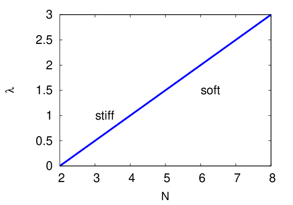
in the limit of large systems, i.e., $L\gg a_{0}$, where $L$ is a lower momentum cut-off $\sim$ linear system size. Regardless of the value of $T_{c}$, () holds as long as $\lambda>\lambda_{c}(\epsilon=0)$. Thus similar to Ref. [3], $\Delta_{0}$ diverges as $L\rightarrow\infty$, but very slowly and remains finite for any finite value of $L$. In contrast for pure NLS, $\kappa(q)$ vanishes for a low enough $q$. Hence for the pure system, $\Delta_{0}$ will diverge even for a finite system size. For $d>2$, it may be shown straightforwardly that $\Delta_{0}$ is finite in TL. Thus, true LRO exists for $d>2$. A phase diagram of the system in the $\lambda-\epsilon$ plane is shown in Fig. 1, with the line of FPs given by $\lambda=\lambda_{c}(\epsilon)$, SRO for $\lambda<\lambda_{c}(\epsilon)$, LRO for $\lambda>\lambda_{c}(\epsilon),\,\epsilon>0$ and stiff phase for $\lambda>\lambda_{c}(\epsilon=0)$ .

It is insightful to consider the flow of the reduced temperature $\tilde{T}=T_{c}/\kappa$ ar $2d$. We find

$$\frac{d\tilde{T}}{dl}=\tilde{T}^{2}[\frac{N-2}{2\pi}-\frac{2\lambda}{2\pi}].$$

(34)

For $\lambda=0$ and $N>2$, $\tilde{T}=0$ is the only DRG FP. This is, however, an unstable FP (expected), such that even for an arbitrarily small (microscopic) $\tilde{T}=\tilde{T}_{0}$, scale-dependent $\tilde{T}(l)$ grows. Integrating (34)

$$-\frac{1}{\tilde{T}}=A_{0}l+C,$$

(35)

where $A_{0}=\frac{N-2}{2\pi}-\frac{2\lambda}{2\pi}$ and $C$ is a constant of integration. Assume $A_{0}>0$. Set at $l=0$, $1/\tilde{T}=1/\tilde{T}_{0}>0$, we have

$$-\frac{1}{\tilde{T}}=A_{0}l-\frac{1}{\tilde{T}_{0}}.$$

(36)

Thus, as $l\rightarrow 1/(A_{0}\tilde{T}_{0})\sim\ln\zeta$ from below, $\tilde{T}\rightarrow\infty$. This implies that for any microscopic $\tilde{T}_{0}>0$, the large scale properties of the system is identical to that of a system at $\tilde{T}\rightarrow\infty$, indicating disordered phase at all $\tilde{T}>0$. Since $T_{c}$ for an Ising system at $2d$ is always larger than zero (there is a finite temperature Ising ferromagnetic phase), our Model I at $T=T_{c}$ is always in its disordered phase for $\lambda=0$. This scenario changes for $A_{0}<0$, or, $\lambda>\lambda_{c}$ at $2d$. Flow equation (34), upon integration, now yields

$$\frac{1}{\tilde{T}}=|A_{0}|l+\frac{1}{\tilde{T}_{0}}.$$

(37)

Evidently, for $l\rightarrow\infty$, $\tilde{T}\rightarrow 0$. Therefore, for $\lambda>\lambda_{c}(\epsilon=0)$, scale-dependent $\tilde{T}(l)$ flows to zero as $l\rightarrow\infty$, where as for $\lambda<\lambda_{c}(\epsilon=0)$, $\tilde{T}(l)$ flows to infinity as $l\rightarrow\ln\zeta$. Thus for $\lambda>\lambda_{c}(\epsilon=0)$, the properties of the system at the largest (formally TL) scale is expected to be same as that of the system at zero temperature. This suggests the existence of order in the system. On the other hand, for $\lambda<\lambda_{c}(\epsilon=0)$, the behavior of the system at large scale is same as that at infinite temperature, indicating a paramagnetic phase with SRO only. Thus, as $\lambda$ rises from 0 to a high value through $\lambda_{c}(\epsilon=0)$, the system undergoes a phase transition from a disordered (paramagnetic) phase to an ordered phase through a critical point at $\lambda=\lambda_{c}(\epsilon=0)$. This is reminiscent of the usual temperature driven order-disorder second order transition; however, in the presence case, $T$ is kept fixed at $T_{c}$ and $\lambda$ is the tuning parameter.

We now discuss the nature of the order in the ordered phase, and whether it is identical to the magnetic (i.e., ferromagnetic) order in usual magnetic systems. The usual magnetic transition is conveniently described by the magnetic order parameter, which is non-zero in the ferromagnetic phase but zero in the paramagnetic phase. Since we assume order in the “1” direction in the spin space, we take $m=\langle\sigma\rangle=\langle\sqrt{1-\pi^{2}}\rangle\approx 1-\langle\pi^{2}\rangle/2$ as the order parameter. Clearly, in the disordered phase $m\approx 0$ for a system with a linear size approaching $\zeta$. Interestingly, even in the ordered phase, $m\approx 0$ in TL, due to the divergences found in $\Delta_{0}$ above; see Eq. (). Thus, $m$ remains zero on both sides of the critical point given by $\lambda=\lambda_{c}$, and hence cannot work as an order parameter here [26]. Instead, we take

$$\overline{O}=[\ln(\xi/a_{0})]^{-1}=-T_{c}\Delta\lambda/(\pi\kappa_{0}),$$

(38)

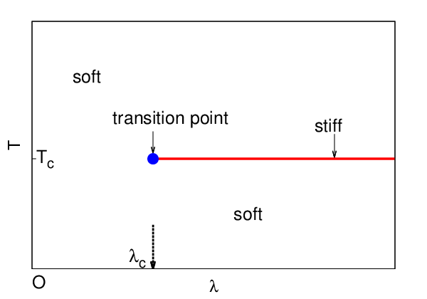
with $\lambda<\lambda_{c}$ and $\overline{O}=0$ with $\lambda\geq\lambda_{c}$ as the order parameter at 2d. This is similar to the order parameter defined in the context of a crumpled to stiff phase of a heterogeneous fluid membrane [3]. Evidently, $\overline{O}$ in the soft phase rises smoothly from zero, as $\lambda$ is reduced from $\lambda_{c}$. Thus, with $\lambda$ as the control parameter, the order parameter exponent is unity. In the stiff phase, $\overline{O}$ is naturally zero. A schematic plot of $\overline{O}$ versus $\lambda$ is shown in Fig. 2. Fig. 3 and Fig. 4 provide schematic phase diagrams of Model I in the $N-\lambda$ (with $T=T_{c}$) and $\lambda-T$ (for a fixed $N>2$) planes at $2d$ [27].

What happens for $N=2$ at $2d$? In pure NLS, the transition temperature becomes indeterminate, suggesting the importance of topological defects and amplitude fluctuations in destroying LRO in the system. When the $O(2)$ spin is coupled to the Ising spin, the flow equation for $\kappa(l)$ reduces to

$$\frac{d\kappa}{dl}=\frac{\lambda T_{c}}{\pi},$$

(39)

giving $\kappa(q)=\kappa_{0}-\lambda T_{c}\ln(a_{0}q)/\pi$ for all $\lambda>0$. Thus for any positive $\lambda$, renormalized $\kappa(l)$ diverges in TL. As a result, $\Delta_{0}\sim[\ln\,\ln L]/\lambda$ at $T=T_{c}$ and the $O(2)$ spins should appear more ordered than the XY model with QLRO at low $T$. In an equivalent picture, (34) for $N=2$ reduces to

$$\frac{d\tilde{T}}{dl}=-\tilde{T}^{2}\frac{\lambda}{\pi}.$$

(40)

Thus, $\tilde{T}(l)$ always flows to zero for all $\lambda>0$. Hence, Model I with $N=2$ is in its ordered stiff phase for all $\lambda$. We now calculate the Debye-Waller factor and the equal-time spin-spin correlation $C_{s}(r)=\langle\Phi({\bf x})\cdot\Phi({\bf x^{\prime}})\rangle$, for $N=2$ in the stiff phase ($T=T_{c},\lambda>\lambda_{c}$), where $r=|{\bf x}-{\bf x^{\prime}}|$ is assumed to be large. For $N=2$, the transverse components $\boldsymbol{\pi}$ has only one component, say, $\tilde{\pi}$; $\Phi$ may be expressed as a complex number $\exp(i\Psi)$ where $\Psi({\bf x},t)$ is a real scalar field; we write $\Phi_{1}=\cos\Psi,\,\Phi_{2}=\sin\Psi$ as the two components of $\Phi$. For small transverse fluctuations in a nearly ordered state, associate $\Psi$ with $\tilde{\pi}$ (equivalently, parametrize $\Phi=\exp(i\tilde{\pi})$; see Appendix D for formulation of the dynamics in terms of $\Psi$). In the renormalized version of Model I, the variance of $\tilde{\pi}({\bf x},t)$ in the stiff phase (for all $\lambda>0$) in $2d$ is given by () with $\epsilon=0$ and $N=2$. Now assuming “1” to be the ordering direction, the average order parameter

	$\displaystyle\langle\cos\Psi\rangle$	$\displaystyle=$	$\displaystyle\exp[-\frac{1}{2}\langle\tilde{\pi}({\bf x},t)^{2}\rangle]=\exp[-\frac{1}{2}\Delta_{0}]$		(41)
		$\displaystyle=$	$\displaystyle\exp[-\frac{1}{4\lambda}\ln|\ln L|]=\exp(-W),$

in (renormalized) Model I for a system of (large) linear size $L$. The Debye-Waller factor that determines the depreciation of the magnetization due to the noise induced fluctuations (thermal fluctuations for equilibrium systems) is given by $\exp(-2W)$, where $2W=\Delta_{0}=(\ln\ln L)/(2\lambda)$ in the limit of large $L$ [9]. Clearly, $W\rightarrow\infty$ in TL here and hence the order parameter vanishes in TL. Note, however, that as $\lambda$ rises, $W$ decreases for a fixed $L$, and thus, an increase in $\lambda$ reduces thermal depreciation of the magnetisation. Furthermore,

	$\displaystyle C_{s}(r)$	$\displaystyle=$	$\displaystyle\langle\cos[{\Psi({\bf x},t)-\Psi(0,t)}]\rangle$
		$\displaystyle=$	$\displaystyle Re\langle\exp(i[\Psi({\bf x},t)-\Psi(0,t)])\rangle=\exp[-g({\bf x})],$

where $g({\bf x})=\langle[\tilde{\pi}({\bf x},t)-\tilde{\pi}(0,t)]^{2}\rangle/2=\int\frac{d^{2}q}{(2\pi)^{2}}[\langle|\tilde{\pi}_{\bf q}(t)|^{2}\rangle[1-\exp(i{\bf q}\cdot{\bf x})]$, where we again have made the association between the phase field $\Phi$ and $\tilde{\pi}$ for small transverse fluctuations. Defining ${\bf q\cdot x}=qr\cos\varphi=u\cos\varphi$, we obtain in renormalized Model I

	$\displaystyle g({\bf x})$	$\displaystyle=$	$\displaystyle-\frac{1}{2\lambda}\int_{rL^{-1}}^{r\Lambda}du\frac{1-J_{0}(u)}{u\ln(ua_{0}/r)}$		(42)
		$\displaystyle=$	$\displaystyle-\frac{1}{2\lambda}\int_{rL^{-1}}^{1}du\frac{1-J_{0}(u)}{u\ln(ua_{0}/r)}+\frac{1}{2\lambda}\int_{1}^{r\Lambda}\frac{duJ_{0}(u)}{u\ln(ua_{0}/r)}$
		$\displaystyle-$	$\displaystyle\frac{1}{2\lambda}\int_{1}^{r\Lambda}\frac{du}{u\ln(ua_{0}/r)},$

where $\Lambda\sim 1/a_{0}$ is an upper momentum cutoff; $J_{0}(u)$ is the zeroth order Bessel function of first kind. Clearly, the first two terms in the last line of (42) remain finite in TL, $L\rightarrow\infty$. Thus in TL for $r\rightarrow\infty$ and neglecting the finite parts

$$g({\bf x})=\frac{1}{2\lambda}\ln|\ln(a_{0}/r)|.$$

(43)

This gives

	$\displaystyle C_{s}(r)$	$\displaystyle=$	$\displaystyle\exp[-\frac{1}{2\lambda}\ln|\ln(a_{0}/r)|]=\frac{1}{|\ln(a_{0}/r)|^{1/2\lambda}}$		(44)
		$\displaystyle=$	$\displaystyle\frac{1}{(\ln r)^{1/2\lambda}},$

in the limit $r\rightarrow\infty$. Thus, the spatial dependence of $C_{s}(r)$ is characterized by a model-dependent exponent $\lambda$, which is reminiscent of QLRO in the XY model below the Kosterlitz-Thouless (KT) transition. Nonetheless, the spatial dependence in (44) is markedly weaker than the algebraic decay of equal-time correlators associated with QLRO [9]. Again for a larger $\lambda$, $g({\bf x})$ is smaller and the spatial decay of $C_{s}(r)$ is accordingly weaker. This is consistent with the role of $\lambda$ in favoring order in the system.

References

- [1] N. D. Mermin and H. Wagner, Phys. Rev. Lett. 17, 1133 (1966); N. D. Mermin, Phys. Rev. 176, 250 (1968).
- [2] Statistical Mechanics of Membranes and Surfaces, edited by D. Nelson, T. Piran, and S. Weinberg World Scientific, Singapore (1989).
- [3] T Banerjee and A Basu, Phys. Rev. E 91, 012119 (2015)
- [4] H.E. Stanley Phys. Rev. Lett. 20 589 (1968).
- [5] B-G. Liu, Phys. Rev. B 45, 10771 (1992); S. Sachdev and M. Vojta, Phys. Rev. B 68, 064419 (2003); A. S. Gliozzi and A. Parola, Phys. Rev. B 64, 184439 (2001); T. Senthil and M. P. A. Fisher, Phys. Rev. B 74, 064405 (2006); K. Borejsza and N. Dupuis Phys. Rev. B 69, 085119 (2004).
- [6] M. Henneaux and A. Wilch, Phys. Rev. D 58, 025017 (1998); A. Alonso-Izquierdo, M. A. G. Leon, and J. M. Guilarte, Phys. Rev. Lett. 101, 131602 (2008); S. Kürk cüoglu, Phys. Rev. D 78, 065020 (2008).
- [7] H. Falomir and E. M. Santangelo, Phys. Rev. Lett. 56, 1659 (1986); S. R. Das and B. Sathiapalan, Phys. Rev. Lett. 57, 1511 (1986).
- [8] H. Kitamoto and Y. Kitazawa, Phys. Rev. D 83, 104043 (2011); J. Lee, T. H. Lee, T. Y. Moon, and P. Oh, Phys. Rev. D 80, 065016 (2009)
- [9] P. M. Chaikin and T. C. Lubensky, Principles of condensed matter physics (Cambridge University Press, Cambridge, 2000).
- [10] U. Täuber, Critical dynamics (Cambridge University Press, Cambridge, 2014).
- [11] S. Banerjee, T. V. Ramakrishnan and C. Dasgupta, Phys. Rev. B 83, 024510 (2011).
- [12] R. Folk, Yu. Holovatch, and G. Moser, Phys. Rev. E 78, 041125 (2008); R. Folk, Yu. Holovatch, and G. Moser, Phys. Rev. E 79 031109 (2009).
- [13] While is a relevant coupling constant in a renormalization group (RG) sense near at ; at the one-loop order, the only effect of is to shift downward; the dynamic exponent and anomalous dimension at the one-loop order at the critical point, same as their values in the linear theory, i.e., with [9, 10]. Hence, treating as the one-loop renormalized , without any loss of generality, we set in what follows below. Effects of a non-zero may be included by considering as the renormalized fields with a non-zero anomalous dimension that becomes non-zero only at ; the dynamic exponent of in a relaxational dynamics is also affected at . Note that the correlation length exponent of gets corrected at the one-loop order, i.e., at . This, however, does not affect out calculations. We have also ignored those contributions to the model parameters defining the dynamics of , which originates from the fluctuations of the spins. These are in comparison with the fluctuation corrections which originate from the fluctuations of itself.
- [14] R. Bausch, H. K. Janssen and Y. Yamazaki, Z. Phys. B 37, 163 (1980).
- [15] C. DeDominicis, J. Phys. (Paris) 37, Colloque C-247 (1976).
- [16] In a dimensional regularization scheme, , see, e.g., Ref. [15].
- [17] Fluctuations of are short lived even for . However, one needs to keep the -term in (3) for thermodynamic stability. We do not discuss this here in details.
- [18] P.Hohenberg and B.Halperin, Rev. Mod. Phys. 49, 435 (1977).
- [19] L. Peliti and S. Leibler, Phys. Rev. Lett., 54, 1690 (1985).
- [20] P. G. de Gennes and J. Prost, The Physics of Liquid Crystals, Clarendon Press (Oxford, 1995).
- [21] M. C. Marchetti, J. F. Joanny, S. Ramaswamy, T. B. Liverpool, J. Prost, M. Rao, and R. A. Simha. Rev. Mod. Phys. 85, 1143 (2013).
- [22] R. Ruiz and D. R. Nelson, Phys. Rev. A 23, 3224 (1981).
- [23] Note that there is a convolution of the terms in the Fourier space which yields the scale factor of along with in Eq. 69.
- [24] Note that the effective dynamical equations for the spins have been written directly, by exploiting the time-scale separations between the fast relaxation of the particle number density fluctuations and the slow relaxation of the broken symmetry fields. As a result, the particle number densities do not appear as separate dynamical variables in the model equations, but as effective noises with symmetry-permitted structures in the equations for spins. The form of these dynamical equations of the spins are, of course, dictated by whether the effective spin dynamics is nonconserved or conserved. The former and latter cases may be viewed as nonequilibrium dynamic analogs of the grand canonical and canonical ensembles for equilibrium systems, respectively.
- [25] M. Kardar, G. Parisi and Y.C Zhang, Phys. Rev. Lett., 56, 889 (1986).
- [26] The absence of LRO at even for is consistent with .
- [27] While the order parameter does distinguish the stiff phase from the soft phase, it is unusual as an order parameter in the sense that it is not defined locally.
- [28] H Hinrichsen, Adv. Phys. 49, 815 (2000).