von Kármán–Howarth and Corrsin equations closure based on Lagrangian description of the fluid motion.

Recently, a work dealing with the bifurcations analysis of the turbulent energy cascade [12] presents, among the other things, the relationship between Navier–Stokes equations bifurcations and turbulent energy cascade, showing that these bifurcations produce a negative value of the skewness of the longitudinal velocity difference, and a separation rate between contiguous trajectories which exponentially diverges with the time.

The present work proposes a specific analysis of the isotropic homogeneous turbulence of incompressible fluids based on Ref. [12], and on the property that the contiguous fluid particles trajectories continuously diverge due to the Navier–Stokes bifurcations. The proposed formulation adopts the Lagrangian representation of the fluid motion and the Liouville theorem.

According to the present study, the bifurcations determine the energy cascade, where the separation vector $\xi$ between two fluid particles trajectories varies much more rapidly than the velocity and temperature [12]. Such property, in conjunction with the hypothesis of fully developed turbulence, justifies the assumption that $\xi$ and the velocity field are statistically independent. This is the crucial hypothesis of the present analysis that allows, through the Liouville theorem, to analytically express the closure formulas of the von Kármán–Howarth and Corrsin equations in terms of longitudinal velocity and temperature correlations. The proposed analysis also quantifies the mean effect of the trajectories separation through the average finite–scale Lyapunov exponent, a quantity depending on $r$ which gives the rate of separation of the trajectories with finite distance. This exponent is here calculated in function of the maximum finite–scale Lyapunov exponent through the distribution function of $\xi$ and the Liouville theorem.

For sake of the reader convenience, we report the main keypoints of the article: The first part of the work, devoted to the Lagrangian description of the fluid motion, provides the representation of velocity and temperature fields, and of the kinematics of a pair of fluid particles. The Liouville theorem is then introduced, and the statistical independence of $\xi$ from velocity and temperature fields is properly justified. In the second part, a relationship between average and maximal Lyapunov exponents of finite–scale, useful for the subsequent analysis, is determined, and the average Lyapunov exponent is expressed in terms of longitudinal velocity correlation. Thereafter, the closure equations are obtained through the analytical elements introduced in the previous two parts.

The obtained results agree with those presented in Refs. [13, 14], where the closure formulas are carried out using a fully different formulation and exploiting some of the properties of motion of the finite–scale Lyapunov basis, and the frame invariance of the triple correlations appearing in the von Kármán–Howarth and Corrsin equations. This corroborates the results obtained in Refs. [13, 14], showing the equivalence between the present approach and the analysis of Refs. [13, 14].

Finally, some of the properties of the closed von Kármán–Howarth and Corrsin equations are studied and their limits of validity are discussed. Specifically, we show that the times of developing of velocity and temperature correlations are both finite quantities which depend on the initial conditions.

In fully developed homogeneous isotropic turbulence, the turbulent fluctuations of velocity and temperature are represented by the following pair correlation functions [21, 10]

where the brackets $\left\langle\right\rangle$ denote the average calculated over the ensemble of velocity and temperature in the points $\bf x$ and ${\bf x}+\bf r$, $u_{r}={\bf u}({\bf x})\cdot{\bf r}/r$ and $u_{r}^{\prime}={\bf u}({\bf x}+{\bf r})\cdot{\bf r}/r$ are the longitudinal components of fluid velocities, $\vartheta$ and $\vartheta^{\prime}$ are the fluid temperatures in $\bf x$ and $\bf x+\bf r$, and $u^{2}=\langle{\bf u}\cdot{\bf u}\rangle/3$, $\theta^{2}=\langle\vartheta^{2}\rangle$ represent the standard deviations of velocity and temperature, both constants in space due to homogeneity [21, 10]. Such correlations vary according to the von Kármán–Howarth and Corrsin equations [21, 4, 10, 11] which are the evolution equations for $f$ and $f_{\theta}$, respectively. These equations, obtained through the momentum Navier–Stokes and the thermal energy equations, are [21, 10]

where $\nu$ and $\chi=k/(\rho C_{p})$ are kinematic viscosity and thermal diffusivity, $C_{p}$ and $k$ are specific heat at constant pressure and thermal conductivity, respectively. The quantities $\lambda_{T}\equiv\sqrt{-1/f^{\prime\prime}(0)}$ and $\lambda_{\theta}\equiv\sqrt{-2/f_{\theta}^{\prime\prime}(0)}$ are the Taylor and Corrsin microscales. The boundary conditions associated to Eqs. (5) and (6) are

In Eqs. (5) and (6), $K$ and $G$ arise from the inertia forces and from the convective terms of the Navier–Stokes and thermal energy equations [21, 10], and can be expressed as

Accordingly, $K$ and $G$ do not modify neither the kinetic energy nor the thermal energy, and provide the energy cascade mechanism the effect of which vanishes for $r=0$ and for $r\rightarrow\infty$, i.e.

In this study, we analyze the case where $\nu$ does not depend on $\vartheta$, therefore Eq. (5) is independent from Eq. (6) and $f_{\theta}$. Conversely, the temperature fluctuations will depend on $\bf u$.

Following the present analysis, the turbulence is caused by the bifurcations of the Navier–Stokes equations, whereas the temperature plays the role of the passive scalar. This study applies also to any passive scalar which exhibits diffusivity. These bifurcations frequentely occur in developed turbulence determining a condition of fully developed chaos where velocity and temperature exhibit chaotic fluctuations, and the contiguous fluid particles trajectories diverge continuously with exponential growth rate [12]. This implies that the fluid deformations are represented by exponential growth functions of the time, whereas the fluid state variables, like velocity and temperature, are slow growth functions of $t$.

The purpose of this section is to present the link between average and maximum Lyapunov exponents of finite–scales that will be useful later on in this analysis.

The average effect of the trajectories divergence is quantified by the average finite–scale Lyapunov exponent, a quantity which expresses the separation rate between two trajectories with finite distance. To define this exponent, observe that the following quantity

gives the local growth rate of $|\mbox{\boldmath$\xi$}|$. Following its definition, the maximal finite–scale Lyapunov exponent gives the maximum growth rate of the trajectories distance. In the present framework, this exponent can be written as

The overline $\displaystyle\overline{\circ}$ denotes the average calculated according to Eq. (3.2), where $\lambda=\lambda(r)$ thanks to the turbulence isotropy. This exponent is associated to a given spatial direction $l_{1}$, variable with the time, which corresponds to the maximum growth rate of trajectories distance.

On the other hand, the trajectories separation happens with a mean growth rate. This latter is defined through the average finite–scale Lyapunov exponent, a quantity calculated as the mean of $\lambda^{\prime}$

If the ergodic hypothesis is satisfied, this average exponent is calculated in terms of the distribution $P$ as

With reference to Fig. 1, the continuous line represents the time variations of $1/2{\ln({\mbox{\boldmath$\xi$}}\cdot{\mbox{\boldmath$\xi$}})}$ and its local slope gives $\lambda^{\prime}$ (dash–dotted line), whereas $\lambda$ and $\overline{\lambda^{\prime}}$ are represented by dashed and dotted lines, respectively.

The two exponents are related with each other, and to express $\overline{\lambda^{\prime}}$ in function of ${\lambda}$, we write $\overline{\lambda^{\prime}}$ in terms of $\partial P/\partial t$

where the first term at the R.H.S. of Eq. (4) identifies $\lambda$, whereas the second one is expressed by means of the Liouville theorem

Integrating by parts the last term at the R.H.S. of Eq. (4), and using the Green’s second identity, we obtain the sum of two terms. The first one of these identically vanishes as it is an integral of $P$ over $\partial\left\{{\mbox{\boldmath$\xi$}}\right\}$ where $P\equiv$ 0, whereas the other one is different from zero. This leads to

Hence, taking into account Eq. (4), we have

Due to homogeneity, the separation rate does not depend on $\bf x$, and thanks to the isotropy $\overline{\lambda^{\prime}}$ and ${\lambda}$ are both even functions of $r$ [4, 31].

Finally, it is worth remarking a property of the function ${\mbox{\boldmath$\chi$}}:{\mbox{\boldmath$\xi$}}(0)\rightarrow{\mbox{\boldmath$\xi$}}$: when $0<t\lesssim 1/\lambda$, $\xi\rightarrow r\exp({\lambda}t)$, thus $\chi$ satisfies the following equation

In order to express $\overline{\lambda^{\prime}}$ in terms of $f$, observe that along the direction $l_{1}$, $\xi$ varies following $\xi=\xi(0)\exp(\lambda t)$, i.e.

where ${\bf Q}(t)$ is a proper rotation matrix which gives the orientation of $\xi$ with respect to the inertial reference frame. Hence, the relative velocity $\dot{\mbox{\boldmath$\xi$}}$ is

where ${\mbox{\boldmath$\omega$}}_{\mbox{\boldmath$\lambda$}}$ is the angular velocity of $\xi$ and $l_{1}$ with respect to the inertial reference.

Now, because of the isotropy, the standard deviation of $\Delta u_{r}$ does not depend on ${\bf r}/r$, and this implies that

Hence, $f$ and $\overline{\lambda^{\prime}}$ are linked with each other according to

Equation (69) is defined only for $f<1$ and this agrees with Schwarz inequality [4], and in particular, for $\partial f/\partial r<$0 near the origin.

In conclusion, in fully developed homogeneous isotropic turbulence, the fluid particles trajectories continuously diverge with an average separation rate $\dot{R}$ which depends on $r$ following

Here, the closure formulas of Eqs. (5) and (6) are determined by means of the elements introduced in the previous sections.

To obtain these formulas, observe that $K$ and $G$ are responsible only for the energy cascade. This latter is the kinetic and thermal energy flow between the length scales, without changing the total amount of kinetic and thermal energy (see for instance [4, 10] and references therein). In fact, inertia and pressure forces and the convective term produce an interaction between the various Fourier components of velocity and temperature spectra which gives the kinetic and thermal energy transfer between the volume elements in the wave–number space, where the global effect of such interaction leaves $u^{2}$ and $\theta^{2}$ unaltered [4, 10].

Now, to determine $K$ and $G$, we first calculate the pair correlations $f$ and $f_{\theta}$ through the PDF $\cal F$, taking into account the initial condition of $P$ given by Eq. (46). Accordingly, longitudinal velocity and temperature correlations can be expressed through ${\cal F}$

or in terms of $F$ as

in which $u_{\xi}={\bf u}\cdot{\mbox{\boldmath$\xi$}}/\xi$. The correlations (6) and (6) are linked with each other because the fluctuation ${\mbox{\boldmath$\chi$}}:$ ${\mbox{\boldmath$\xi$}}(t^{-})$ $\rightarrow$ $\mbox{\boldmath$\xi$}(t)$, ${\mbox{\boldmath$\xi$}}(t^{-})={\bf r}$, $t=t^{-}+\varepsilon$, $\varepsilon>0$ varying much more rapidly than $f$ and $f_{\theta}$, leaves unaltered the correlations in the transformed points, therefore, taking into account Eq. (65), we have $f(t,\xi)$=$f(t^{-},r)$, $f_{\theta}(t,\xi)$=$f_{\theta}(t^{-},r)$, and

Hence, the time derivatives of the correlation functions are calculated by means of $\partial{\cal F}/\partial t$, using Eq. (3.3)

As previously seen, the terms with $\partial F/\partial t$ correspond to the time variations of kinetic and thermal energies and to the changing of the correlations caused by viscosity and thermal conductivity, whereas those with $\partial P/\partial t$, arising from the fluctuations of $\xi$, do not modify neither $u^{2}$ nor $\theta^{2}$. This identifies $K$ and $G$ as

where $\partial P/\partial t$ is expressed through the Liouville theorem (3.2)

Next, integrating by parts the R.H.S. of Eq. (6), and using the Green’s second identity, we obtain that both $K$ and $G$ are the sum of two terms. The first ones identically vanish as these are integrals of $P$ over $\partial\left\{{\mbox{\boldmath$\xi$}}\right\}$ in which $P\equiv$ 0, whereas the other ones are different from zero. This leads to

Taking into account the turbulence isotropy, and Eq. (6), we obtain

It is worth remarking that $\dot{\mbox{\boldmath$\xi$}}$, depending on $x$ and $\xi$, is considered to be a fast variable, thus its contribution is calculated with the statistics of $P$. This leads to express $K$ and $G$ in terms of $\partial f/\partial r$ and $\partial f_{\theta}/\partial r$

Hence, in view of Eqs. (4) and (69), we obtain the following expressions

Following Eqs. (6), the phenomenon of kinetic and thermal energy cascade is due to the combined action of the spatial variations of $f$, $f_{\theta}$ and of the trajectories separation. Therefore, $K$ and $G$ result to be non–monotonic even functions of $r$ which vanish for $r=0$ and tend to zero as $r\rightarrow\infty$. In particular, $K$ gives also the values of the skewness of $\partial u_{r}/\partial r$ [13] which is constant and is equal to $-3/7$. Table 1 reports the comparison between the value of the skewness

calculated with the proposed expression of $K$ and those obtained by the several authors with direct numerical simulation of the Navier–Stokes equations (DNS), and Large–eddy simulations (LES). It results that the maximum absolute difference between the proposed value and the other ones results to be less than 10 $\%$. Other comparisons between the proposed closure formulas and the results of the literature can be found in the previous works [13, 14, 15].

Equations (6) coincide with those obtained in Refs. [13, 14] through the properties of the motion of the finite–scale Lyapunov basis and of the frame invariance of $K$ and $G$. This shows that the hypotheses adopted in Refs. [13, 14] agree with the assumptions of the present analysis.

The main asset of Eqs. (6) with respect to the other models is that Eqs. (6) are not based on phenomenological assumptions, such as for instance, the existence of the eddy viscosity [23, 24, 26, 16, 3, 32], but are obtained through theoretical considerations regarding the statistical independence of $\xi$ from $\bf u$, and the Liouville theorem. Thanks to their theoretical foundation, Eqs. (6) do not incorporate free model parameters or empirical constants which have to be identified.

Refs. [13, 14] show that such formulas describe adequately the energy cascade mechanisms. Specifically, $K$ reproduces the phenomenon of kinetic energy cascade in line with the Kolmogorov law, and $G$ describes the thermal energy cascade according to the theoretical argumentation presented in the Refs. [5, 6, 27], to experimental results [22, 25], and to numerical data [8, 17].

$K$ and $G$ arise from inertia forces and convective term, thus these do not depend on $\nu$ and $\chi$. Specifically, $K$ and $G$ are only indirectly related to $\nu$ and $\chi$ through $f$ and $f_{\theta}$ whose time evolutions depend on diffusivities by means of Eqs. (5) and (6).

Finally, we remark the limits of the proposed equations. Such limits arise from the hypotheses under which Eqs. (6) are derived: Eqs. (6) hold only in regime of fully developed turbulence where the flow statistical properties exhibit homogeneity and isotropy. Otherwise, during the transition through the intermediate stages of the turbulence, in decaying turbulence, or in more complex situations of developed turbulence with boundary conditions, for instance in the presence of wall, Eqs. (6) can not be applied.

Remarks. Observe that, thanks to the Navier–Stokes bifurcations, the proposed closure formulas modify significantly the mathematical structure of Eqs. (5) and (6).

In Refs. [19, 20], the authors, studying the non–closed von Kármán–Howarth equation by group theoretical methods, suggest solutions to the closure problem of isotropic turbulence, especially for what concerns the decay of the turbulence. Their two works were not based on the Navier–Stokes bifurcations, and their proposed closure formulas exhibit symmetries. Here, Eqs. (6) may not present such symmetries, and this is due to the Navier–Stokes bifurcations which determine the continuous trajectories divergence and thus the possible absence of these symmetries.

This section analyzes some of the properties of the closed Corrsin and von Kármán–Howarth equations, with particular reference to the evolution times of the developed kinetic energy and temperature spectra. In particular, we will show that these spectra reach their developed shape in finite times which depend on the the initial condition and on the classical maximal Lyapunov exponent $\Lambda$.

The exponent $\Lambda$ is linked to $\lambda$ through

and can be calculated with Eq. (69) considering that, near the origin $f$ and $f_{\theta},$ behave like

Hence

Now, with reference to von Kármán–Howarth and Corrsin equations, $u$ and $\theta$ decrease with $t$ according to [21, 10]

whereas the correlation scales change following these equations

where Eqs. (7) and (7) are, respectively, the equations for the coefficients of the powers $r^{0}$ and $r^{2}$ of von Kármán-–Howarth and Corrsin equations. Equations (7) include the terms with $f^{IV}(0)$ and $f_{\theta}^{IV}(0)$ whose determination requires the equations for the coefficients of the power of $r$ higher than 2. Therefore, we qualitatively discuss the variation laws of the correlation scales and of the classical Lyapunov exponent. The first terms at the R.H.S. of Eqs. (7) are responsible for the energy cascade, whereas the other ones are due to viscosity and thermal diffusivity. For what concerns the energy cascade, it tends to reduce the correlations scales, and if this is sufficiently stronger than viscosity and thermal diffusivity effects, then $d\lambda_{T}/dt<0$ and $d\lambda_{\theta}/dt<0$. On the contrary, the diffusivities tend to increase the correlation scales, thus $f^{IV}(0)$ and $f_{\theta}^{IV}(0)$ are expected to be positive quantities.

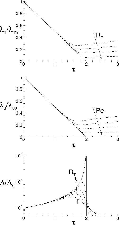
For sake of our convenience, the condition $\nu$=0, $\chi$=0 is first analyzed. In this case, $u$ and $\theta$ are both constants, whereas $\lambda_{T}$, $\lambda_{\theta}$ and $\Lambda$ vary with $t$. From Eqs. (7) and (116), $\lambda_{T}$ and $\lambda_{\theta}$ are proportional with each other, and vary linearly with the time according to

where $\tau$ is the dimensionless time. Therefore, for $\nu$=0, $\chi$=0, the energy cascade described by Eqs. (6) determines the decreasing of the Corrsin and Taylor scales until to $\tau\rightarrow 2$, where both the spectra are considered to be fully developed, and $\lambda_{T}\rightarrow 0$, $\lambda_{\theta}\rightarrow 0$ and $\Lambda\rightarrow\infty$ (see solid lines of Fig. 2). That is, the correlation functions exhibit developed shapes in a finite time whose value depends on the initial condition $\Lambda(0)$. The correlations scales are decreasing functions of $\tau$ whereas $u$ and $\theta$ are both constants, and this means that mechanical and thermal energies are transfered from large to small scales.

For $\nu>$0, $\chi>$0, $du/d\tau<$0 and $d\theta/d\tau<$0, therefore $f$ and $f_{\theta}$ are considered to be fully developed when $d\lambda_{T}/dt=0$ and $d\lambda_{\theta}/dt=0$, respectively. These cases are qualitatively represented by the dashed lines for different values of $R_{T}$ and $Pe$, where $R_{T}=\lambda_{T}u/\nu$, $Pe=PrR_{T}$ and $Pr=\nu/\chi$ are, respectively, the Reynolds number and the Péclet number, both referred to the Taylor scale, and the Prandtl number. If the initial values of $\lambda_{T}$ and $\lambda_{\theta}$ are relatively high, the dissipation effects are quite small in comparison with those of the convective terms. Accordingly, the phenomenon of energy cascade is initially stronger than the diffusivities effects, and this determines that $\lambda_{T}$ and $\lambda_{\theta}$ diminish exhibiting about the same trend of the case $\nu=\chi$=0. Following Eqs. (7) and (7), the interval of $\tau\in(0,2)$ can be splitted in two regions for $f$ and $f_{\theta}$. The first ones occur where $d\lambda_{T}/d\tau<$0, $d\lambda_{\theta}/d\tau<$0 until to certain values of $\tau_{1}<$2, $\tau_{2}<$2, in which $d\lambda_{T}/dt(\tau_{1})=0$, $d\lambda_{\theta}/dt(\tau_{2})=0$ (dashed lines) where, in general, $\tau_{1}\neq\tau_{2}$. In this last situation, the mechanism of energy cascade is balanced by viscosity and thermal diffusivity, and the turbulent spectra can be considered to be fully developed. In any case, this happens in finite times $\tau<$2 for the two spectra. The Lyapunov exponent initially coincides about with that calculated for $\nu=$0, then reaches its maximum for $\tau_{1}<2$ and thereafter diminishes due to the viscosity effects. When $\Lambda$ reaches its maximum, $d\Lambda/d\tau=$0, it is reasonable that chaos and mixing achieve their maximum level, and the spectra are there considered to be fully developed.

Thereafter, we observe the region where $d\Lambda/d\tau<$0. There, due to the smaller values of $\lambda_{T}$ and $\lambda_{\theta}$, the dissipation is stronger than the energy cascade, and $\lambda_{T}$ and $\lambda_{\theta}$ tend to rise according to Eq. (7). This region, which occurs immediately after the fully developed condition ($d\Lambda/d\tau=$0), corresponds to the decaying turbulence regime.

It is worth to remark that the proposed closure equations (6) are expected to be valid in the region where $d\Lambda/d\tau>$0, where the effects of the Navier–Stokes bifurcations generate the regime of fully developed turbulence. On the contrary, for decaying turbulence, $d\Lambda/d\tau<$0, after a certain time, say $\tau^{+}\gtrsim\tau_{1}$, the regime of decaying turbulence may not correspond to the fully developed turbulence, and Eqs. (6) are not defined.

In the case of complete self–similarity, the several solutions of Eqs. (5)–(6) are congruent with each other by proper scale factors depending on only one of the variables. Thus, the von Kármán–Howarth and Corrsin equations are reduced to be ordinary differential equations, and this happens when [11, 21]

On the other hand, the proposed closure formulas can not be brought to Eqs. (7), thus Eqs. (6) do not give a complete self–preservation. Nevertheless, in the cases in which the dimensionless quantities of Eq. (7) exhibit relatively slow variations with respect to the correlations, the solutions can be considered to be self–preserved only in first approximation. In this case, the correlations read as

Next, from Eq. (7) we have

and $f^{IV}$ is proportional to $f_{\theta}^{IV}$ according to Eq. (7)

Hence, the correlations are considered to be fully developed when $\tau^{*}=\tau_{1}=\tau_{2}$. There, $f^{IV}(0,t^{*})$ is linked to $\lambda_{T}(t^{*})$ through Eq. (7) with $d\lambda_{T}/dt$=0 [15]

We conclude this section by observing that the times of developing of $f$ and $f_{\theta}$ are finite quantities which depend on the initial conditions.

In order to obtain the closure formulas for von Kármán–Howarth and Corrsin equations, this analysis represents the fluid motion in the Lagrangian form. As the separation vector varies much more rapidly than the velocity field, $\xi$ and (${\bf u},\mbox{\boldmath$\vartheta$}$) are assumed to be statistically independent. This conjecture and the adoption of the Liouville theorem lead to the closure of von Kármán–Howarth and Corrsin equations. The equations here obtained coincide with those of the previous study [13, 14], showing that the approach of Refs. [13, 14], dealing with the frame invariance of $K$ and $G$ and the properties of the finite–scale Lyapunov basis, is in agreement with the present analysis. This corroborates the previous works, providing a demonstration of the closure formulas completely different with respect to the previous articles.

Thereafter, some of the properties of these equations are studied. In particular, we show that the condition of developed spectra (correlations) in isotropic homogeneous turbulence is reached in finite times whose values depend on the initial conditions.

This work was partially supported by the Italian Ministry for the Universities and Scientific and Technological Research (MIUR), and received no specific grant from any funding agency in the public, commercial or not-for-profit sectors.

References

- [2] Anderson R., Meneveau C., Effects of the similarity model in finite-difference LES of isotropic turbulence using a lagrangian dynamic mixed model, Flow Turbul. Combust., 62, pp. 201–225, 1999.
- [3] Baev M. K. & Chernykh G. G., On Corrsin equation closure, Journal of Engineering Thermophysics, 19, pp. 154–169, no. 3, DOI: 10.1134/S1810232810030069
- [4] Batchelor G.K., The Theory of Homogeneous Turbulence. Cambridge University Press, Cambridge, 1953.
- [5] Batchelor, G. K., Small-scale variation of convected quantities like temperature in turbulent fluid. Part 1. General discussion and the case of small conductivity, Journal of Fluid Mechanics, 5, 1959, pp. 113–133
- [6] Batchelor G. K., Howells I. D., Townsend A. A., Small-scale variation of convected quantities like temperature in turbulent fluid. Part 2. The case of large conductivity, Journal of Fluid Mechanics, 5, 1959, pp. 134–139
- [7] Carati D., Ghosal S., Moin P., On the representation of backscatter in dynamic localization models, Phys. Fluids, 7(3), pp. 606–616, 1995.
- [8] Chasnov, J., Canuto V. M., Rogallo R. S., Turbulence spectrum of strongly conductive temperature field in a rapidly stirred fluid. Phys. Fluids A, 1, pp. 1698-1700, 1989, doi:10.1063/1.857535.
- [9] Chen S., Doolen G.D., Kraichnan R.H., She Z-S., On statistical correlations between velocity increments and locally averaged dissipation in homogeneous turbulence, Phys. Fluids A, 5, pp. 458–463, 1992.
- [10] Corrsin S., The Decay of Isotropic Temperature Fluctuations in an Isotropic Turbulence, Journal of Aeronautical Science, 18, pp. 417–423, no. 12, 1951.
- [11] Corrsin S., On the Spectrum of Isotropic Temperature Fluctuations in an Isotropic Turbulence, Journal of Applied Physics, 22, pp. 469–473, no. 4, 1951., DOI: 10.1063/1.1699986.
- [12] de Divitiis N., Bifurcations analysis of turbulent energy cascade, Annals of Physics, (2015), DOI: 10.1016/j.aop.2015.01.017.
- [13] de Divitiis N., Lyapunov Analysis for Fully developed Homogeneous Isotropic Turbulence, Theoretical and Computational Fluid Dynamics, (2011) DOI: 10.1007/s00162-010-0211-9.
- [14] de Divitiis N., Finite Scale Lyapunov Analysis of Temperature Fluctuations in Homogeneous Isotropic Turbulence, Appl. Math. Modell., (2014), DOI: 10.1016/j.apm.2014.04.016.
- [15] de Divitiis N., Self–Similarity in Fully Developed Homogeneous Isotropic Turbulence Using the Lyapunov Analysis, Theoretical and Computational Fluid Dynamics, (2012), DOI: 10.1007/s00162-010-0213-7.
- [16] Domaradzki J. A., Mellor G. L. , A simple turbulence closure hypothesis for the triple-velocity correlation functions in homogeneous isotropic turbulence, Jour. of Fluid Mech., 140, 45–61, 1984.
- [17] Donzis D. A., Sreenivasan K. R., Yeung P. K., The Batchelor Spectrum for Mixing of Passive Scalars in Isotropic Turbulence, Flow, Turbulence and Combustion, 85, pp. 549–566, no. 3–4, DOI: 10.1007/s10494-010-9271-6
- [18] Kang H.S., Chester S., Meneveau C. , Decaying turbulence in an active–gridgenerated flow and comparisons with large–eddy simulation., J. Fluid Mech. 480, pp. 129–160, 2003.
- [19] Khabirov S.V., Unal G., Group analysis of the von Kármán-–Howarth equation. Part I. Submodels., Communications in Nonlinear Science and Numerical Simulation. 7, 3, 18, 2002.
- [20] Khabirov S.V., Unal G., Group analysis of the von Kármán-–Howarth equation. Part II. Physical invariant solutions, Communications in Nonlinear Science and Numerical Simulation. 7, 19, 30, 2002.
- [21] von Kármán, T. & Howarth, L., On the Statistical Theory of Isotropic Turbulence., Proc. Roy. Soc. A, 164, 14, 192, 1938.
- [22] Gibson, C. H., Schwarz W. H., The Universal Equilibrium Spectra of Turbulent Velocity and Scalar Fields, Journal of Fluid Mechanics, 16, 1963, pp. 365–384
- [23] Hasselmann K., Zur Deutung der dreifachen Geschwindigkeitskorrelationen der isotropen Turbulenz, Dtsch. Hydrogr. Z, 11, 5, 207-217, 1958.
- [24] Millionshtchikov M., Isotropic turbulence in the field of turbulent viscosity, JETP Lett., 8, 406–411, 1969.
- [25] Mydlarski, L., Warhaft, Z., Passive scalar statistics in high-Péclet-number grid turbulence, Journal of Fluid Mechanics, 358, 1998, pp. 135–175
- [26] Oberlack M., Peters N., Closure of the two-point correlation equation as a basis for Reynolds stress models, Appl. Sci. Res., 51, 533–539, 1993.
- [27] Obukhov, A. M., The structure of the temperature field in a turbulent flow. Dokl. Akad. Nauk., CCCP, 39, 1949, pp. 391.
- [28] Orszag S.A., Patterson G.S., Numerical simulation of three-dimensional homogeneous isotropic turbulence., Phys. Rev. Lett., 28, 76–79, 1972.
- [29] Ottino, J. M., Mixing, Chaotic Advection, and Turbulence., Annu. Rev. Fluid Mech. 22, 207–253, 1990.
- [30] Panda R., Sonnad V., Clementi E. Orszag S.A., Yakhot V., Turbulence in a randomly stirred fluid, Phys. Fluids A, 1(6), 1045–1053, 1989.
- [31] Robertson H. P., The invariant theory of isotropic turbulence, Math. Proc. of the Cambridge Ph. Soc., 36, 209-223, 1940.
- [32] Thiesset F., Antonia R. A., Danaila L., and Djenidi L. , Kármán–Howarth closure equation on the basis of a universal eddy viscosity, Phys. Rev. E, 88, 011003(R), 2013, doi: 10.1103/PhysRevE.88.011003.
- [33] Truesdell, C. A First Course in Rational Continuum Mechanics, Academic, New York, 1977.
- [34] Tsinober, A. An Informal Conceptual Introduction to Turbulence: Second Edition of An Informal Introduction to Turbulence, Springer Science & Business Media, 2009.