The graph spectrum of barycentric refinements
Abstract.
Given a finite simple graph , let be its barycentric refinement: it is the graph in which the vertices are the complete subgraphs of and in which two such subgraphs are connected, if one is contained into the other. If are the eigenvalues of the Laplacian of , define the spectral function on the interval , where is the floor function giving the largest integer smaller or equal than . The graph is known to be homotopic to with Euler characteristic and . Let be the sequence of barycentric refinements of . We prove that for any finite simple graph , the spectral functions of successive refinements converge for uniformly on compact subsets of and exponentially fast to a universal limiting eigenvalue distribution function which only depends on the clique number respectively the dimension of the largest complete subgraph of and not on the starting graph . In the case , where we deal with graphs without triangles, the limiting distribution is the smooth function . This is related to the Julia set of the quadratic map which has the one dimensional Julia set and satisfies as the Laplacians satisfy such a renormalization recursion. The spectral density in the case is then the arc-sin distribution which is the equilibrium measure on the Julia set. In higher dimensions, where the limiting function still remains unidentified, appears to have a discrete or singular component. We don’t know whether there is an analogue renormalization in . The limiting distribution has relations with the limiting vertex degree distribution and so in 2 dimensions with the graph curvature distribution of the refinements .
Key words and phrases:
Spectral graph theory, Barycentric subdivision, Julia sets1991 Mathematics Subject Classification
Primary: 05C50, 57M15, 37Dxx1. Introduction
The spectral theory of graphs [6, 43, 1, 7, 42, 47]
parallels to a great deal the spectral theory of compact Riemannian manifolds
[4, 44, 3]. There are areas with a good match like
inverse spectral topics, heat kernel related topics like Hodge theory where
the dimension of the space of harmonic solutions for example
is the number of connected components and more generally, harmonic -forms are
related to the k’th cohomology groups in a rather explicit way as applying
the heat flow to forms converges to harmonic forms. This can be used for example to
construct the Hurewicz homomorphism from to the cohomology groups by applying the
heat flow on a -form supported initially on a -sphere representing an element in
the homotopy group . It leads to a harmonic -form representing a homology
class. Discrete McKean-Singer [26]
illustrates further, how the graph theory
parallels the continuum [40]: the super trace of the heat kernel for
is the super trace of which is the definition of the Euler characteristic, while
in the case , it counts the alternating sum of the Betti numbers, which by Euler-Poincaré
is the same. The cohomology of discretizations of manifolds has since
the beginning of the development of algebraic topology been used to compute the cohomology
of the manifold. For the convergence of the spectrum of -form Laplacians of a compact
connected Riemannian manifold of dimension , Mantuano’s theorem
[39] tells that for any discretization given by a graph,
the spectra of the Hodge Laplacians are related by
, where the constants
only depend on dimension , the maximal curvature and radius of injectivity of . Also for eigenfunctions,
the number of nodal regions of the eigenfunction is bound by a theorem of
Fiedler [11] by , paralleling the Courant nodal theorem.
The ground state energy is estimated in the same way from below by the Cheeger constant.
The nodal regions on geometric graphs correspond to Chladni figures on compact Riemannian manifolds.
Also in topology like for Brouwer-Lefshetz [27] or Jordan-Brouwer theory [34],
the notions translate nicely to the discrete and barycentric refinements help.
There are also places, where things are different: the Weyl law relating the growth of the eigenvalues with volume
has no direct discrete analogue because the spectrum of a graph is a finite set.
Similarly, the Minashisundaram-Plejel zeta function of a manifold needs
analytic continuation in the continuum, while in the graph case, the zeta function is an entire function.
Already in the case of a circle, where the Dirac version of that zeta function is the Riemann
zeta function, the zeros of the discrete analog on circular graphs can be analyzed well, unlike in the
continuum, where it it is the Riemann hypothesis.
The convergence of the roots [36] of the graph zeta functions is a limit when looking at barycentric
subdivisions of circular graphs, which is also important for
Jacobi matrices generalizing graph Laplacians [41, 14] which we studied in [22]
in an ergodic setup, where the limiting operators are almost periodic Jacobi matrices
over the von Neumann-Kakutani system. The later is the unique fixed point of the 2:1 integral extension operation
in ergodic theory. The hull of the operators is the compact Abelian group of dyadic integers, where space
translation is addition by 1 and where the renormalization step is the shift.
We look now at higher dimensional analogue questions to these one dimensional Jacobi spectral problems.
There are other analogies between Schrödinger operators and geometric Laplacians: while isospectral
deformations are possible in the former case, geometric Laplacians are harder to deform as the isospectral
set of geometries is discrete in general. Having worked with isospectral deformations of Jacobi matrices
in [20, 19] we looked in [21] at higher dimensions and noted that writing can enable
isospectral deformation and break the spectral rigidity. Much later, we realized
that in the Riemannian as well as in the graph case, one can deform the exterior derivative
[30, 29] in an isospectral way. The Riemannian case is a bit more
technical in that story as the deformed exterior derivatives are pseudo differential equations in the
continuum but they satisfy so that
they deform cohomology. The deformation does not affect the Laplacian , but in the complex, the
nonlinear deformation becomes asymptotic to the wave evolution. Interestingly, both in the discrete as well as in the
continuum, space expands, with an inflationary start. This is not artificially placed into the model,
but is a basic property if one lets the Dirac operator move freely in its symmetry group.
Graphs can serve as a laboratory to test concepts related to physics. It is reasonable for example to see
the evolutions of the various differential forms under the wave dynamics as manifestations
of different forces. It is a caricature for physics, where nothing has put into the system except
for geometry, which is a Riemannian manifold in the continuum and a graph in the discrete.
When answering the question which graph to take, symmetry again could give a hint: take a scale invariant graph.
While impossible to achieve in a finite discrete structure, taking
a graph which is multiple way refined in a barycentric way comes close. Not only are parts of the graph
homeomorphic to the entire graph, but also the nerve graphs of open covers are homeomorphic to the entire graph.
This motivates to look at refinements and its spectral properties.
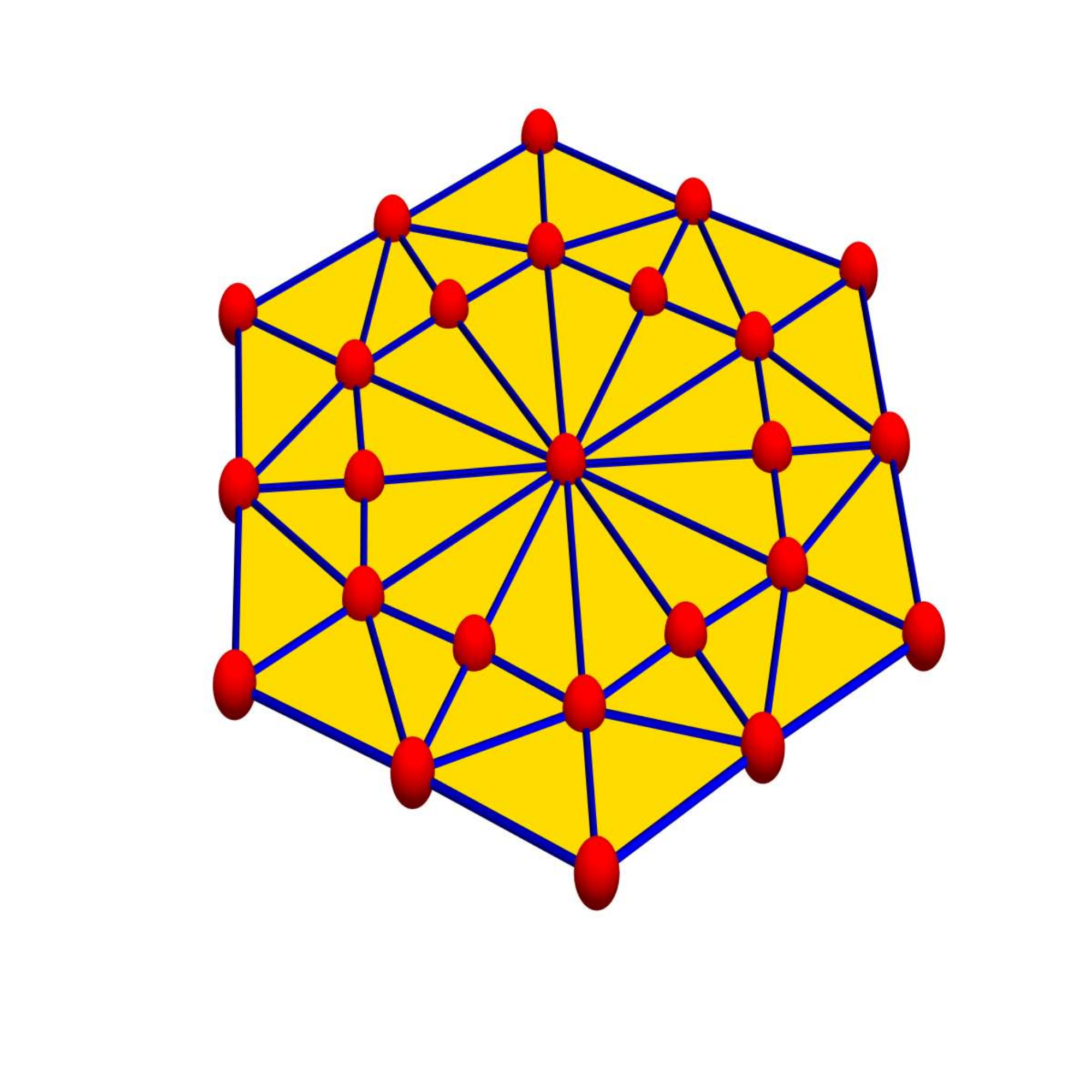
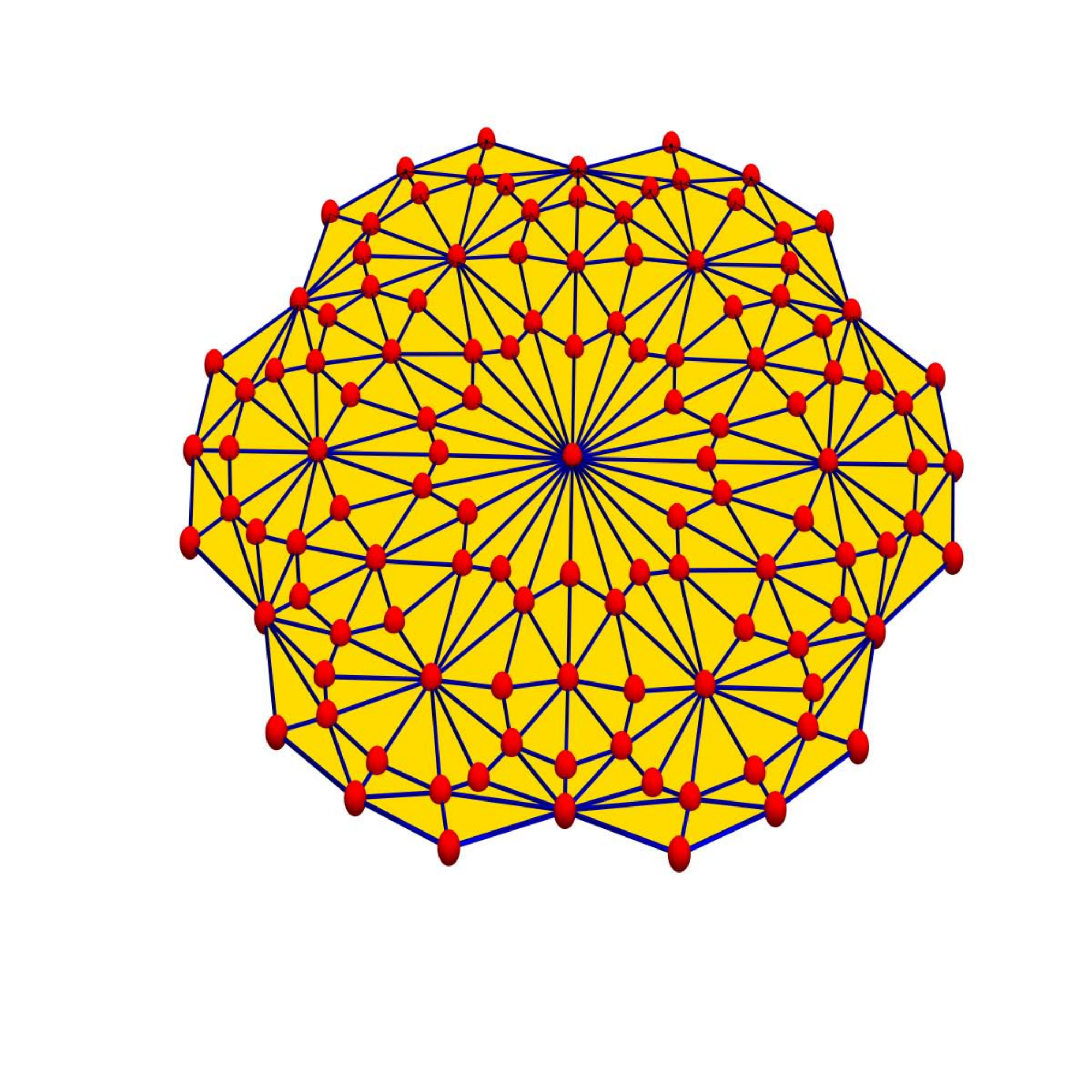
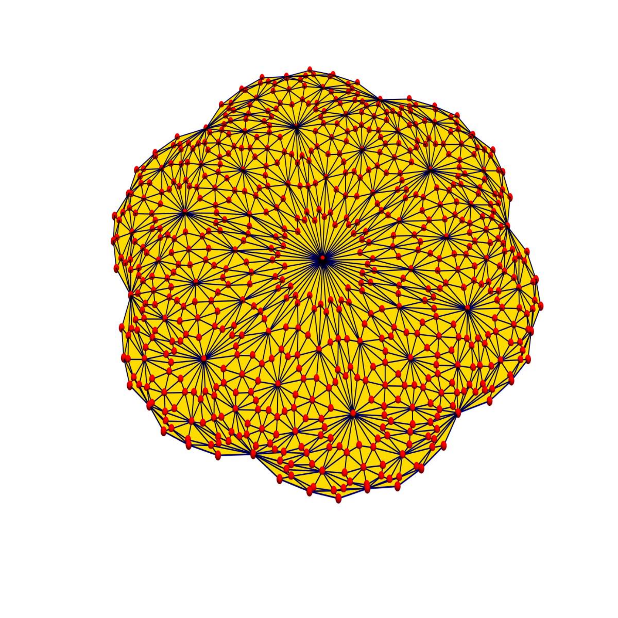
In [35], we looked at a product of graphs which satisfies the same Künneth formula for cohomology as in the continuum. This product of and is defined as follows: take two disjoint unions of and . Pick a complete subgraph of and a complete subgraph of . Let be the complete subgraph generated by . These points form the vertices of . Two such vertices and are connected if one is contained in the other. A special case is if in which case is the barycentric refinement of : its vertices are the complete subgraphs of and two complete subgraphs are connected if one is contained in an other. The graph is homotopic to . It especially has the same Euler characteristic. The dimension of is bounded below by the dimension of . If is geometric, then is even homeomorphic to and the dimensions of and are the same. For any -dimensional geometric , the graphs are all -colorable, the color being the dimension of the original simplices which make up now the vertices. The automorphism group of also acts on so that fixed points of graph automorphisms [27] can be realized as vertices in . Barycentric refinements again stress the point of view taken by discrete Morse theory [12, 13] that complete subgraphs in a graph can be treated as “points”.


For practical triangulations, barycentric refinements are rarely used. The reason is the huge difference
between the possible vertex degrees, as each refinement doubles the maximal degree. But the appearance of
large vertex degrees has also benefits: for any , the graphs are Eulerian with Eulerian spheres
and have the property that a natural geodesic flow can be defined on them in any dimension. This is essential,
as spheres and lines are important in any geometry and that for defining lines, we need an Eulerian property as with an odd
degree vertex, the continuation of a “straight line” is ambiguous: we have difficulty for example to continue
a line through a vertex of an icosahedron as we will have to chose what direction to continue. For graphs in
which all spheres and all spheres in spheres are Eulerian, there is a natural continuation. Graph products and
especially barycentric refinements have this property.
The large and nonuniform degree of some density distributed vertices has the advantage as it allows to emulate
the rotational symmetry in the discrete. For a -dimensional graph, and considering ,
we can in dimension start with a vertex degree of directions. Unlike in regular
lattices or tessellations, the spheres appear more rounded and the fact that the unit sphere
has asymptotically a similar amount of directions than the number of vertices in gives us the property
that the exponential map from the unit sphere to the graph, covers most of the graph.
This is probably the closest we can get to a Hopf-Rynov property in the discrete without digressing into the
quantum (as nature does) and look at the wave equation for the Hodge Laplacian ,
which because has the d’Alembert solution , a superposition
of wave group solutions of the Schroedinger equation
with for the Dirac operator (see [28]) for which
Hopf-Rynov is just linear algebra in the graph case as the unitary group is finite dimensional and
for any two vertices one can solve the problem to start a geodesic on and reach
by choosing the correct velocity and time .


Iterated barycentric subdivisions have long been used in topology and homology theory.
The notion is mostly defined in geometric realizations used to refine a given triangulation of
a simplex in Euclidean space.
Note that we don’t look at any embedding in an Euclidean space but look at Barycentric
refinement in a completely combinatorial setup.
There are also probabilistic connections [8, 15],
as iterated barycentric subdivisions of a triangle define a random walk on and
are linked to concrete geometric properties like angles triangles. Such work could suggest that unlike in the
one dimensional case, in higher dimensions, higher dimensional group actions and random walks
could play a role when studying the spectrum. In graph theory, where no embedding into an Euclidean
space is required, barycentric subdivisions are known in the context of flag complexes
or Whitney complexes in particular. We are not aware of any work on the nature of the spectrum of
such graphs.
The inductive dimension of a graph is defined inductively as the average of the dimensions of all unit
spheres, incremented by [25, 23].
A graph is a geometric -dimensional graph, if every unit sphere is a
-sphere or a -ball and the boundary set of vertices with a ball unit sphere
form a -dimensional geometric graph without boundary.
Geometric graphs play the role of manifolds with or without boundary.
The definition of graph theoretical spheres and homotopy are both due to Evako.
We have defined spheres independently in [33, 35] but realized in
[34] that it is already in the work of Ivashchenko=Evako
[17, 16, 9, 10]. The definition of these Evako spheres is based on Ivashchenko homotopy
which is homotopy notion inspired by Whitehead [48] but defined for graphs.
A simplification done in [5] makes this homotopy much more practical, like for Lusternik-Schnirelman
theory for graphs [18], to define what a homeomorphism for graph is [32] or
for graph colorings [31, 33], where constructing an Eulerian 3 sphere
having a given 2 sphere embedded could explain why 4 colors are enough to color a planar graph.
We proved in [35] the inequality ,
which holds for all finite simple graphs .
This implies in a special case , still for all finite simple graphs .
In the geometric case, the dimension of is the same as the dimension of .
The barycentric refinement process honors geometric graphs, graphs for which the unit spheres are spheres.
Starting with a -simplex , successive refinements
produce geometric graphs which are -balls, for which the boundary is a -sphere. In the
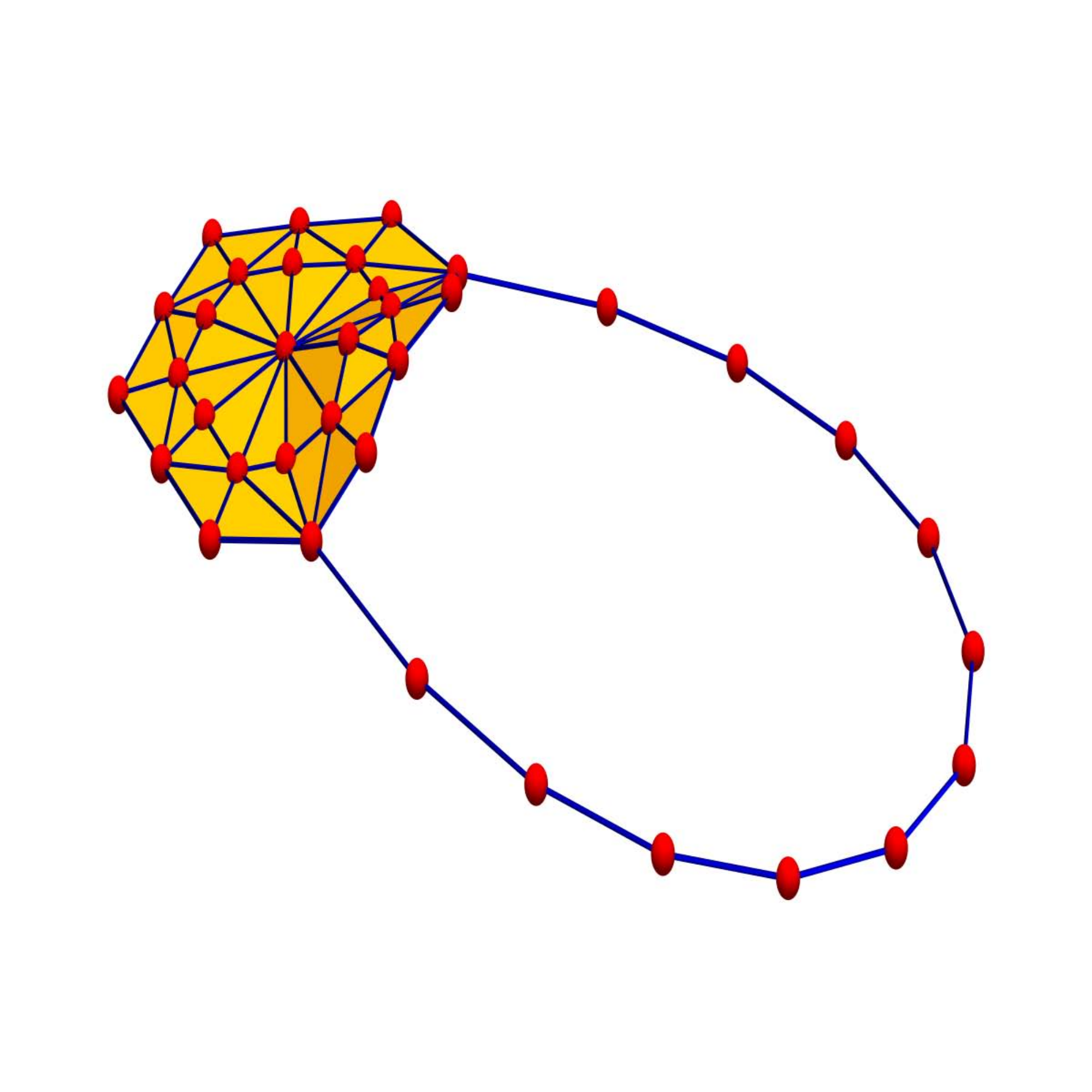
case of a triangle for example, the graph is a wheel graph with spikes. It has one interior point and
boundary point. Successive refinements produce larger and larger balls for which the boundaries are
spheres.
If is a geometric -dimensional graph, then is homeomorphic to in the sense of [32]: there is an open cover of such that the nerve graph of is . To see this, start with unit disks centered at the vertices of which originally were vertices. Then add to the -simplices on the outside which contain simplex in and a vertex simplex . This produces . Two different intersect in a -simplex, if and only the original vertices were connected. Homeomorphic graphs have the same topological properties like cohomology, fundamental groups or connectivities. We furthermore know that for any starting point , the dimension of converges to the dimension of the largest complete subgraph in [35] and the reason is the same as for the spectral convergence studied here: the largest dimensional simplices dominate.
2. Counting
The refinements grow exponentially fast already in the -dimensional case, where the number of edges doubles exactly in each step.
Lemma 1.
a) For , and .
b) For , the number of vertices ,
the number of edges is and the number of triangles
.
c) For , we have and .
Proof.
a) We have as . Furthermore
.
b) From the affine recurrence given by
and with
we get the exact simplex data formula
which in the first coordinate gives the above sequence which grows like .
c) follows from the fact that in each step, a -dimensional simplex is cut into simplices. This shows . Furthermore . ∎
In [46], a combinatorial interpretation of the eigenvalues are given. We hope it will be possible to get also exact formulas for if if . To do so, one could use the handshaking relation (see [24])
where are the number of -dimensional complete subgraphs in the unit
sphere . In the case , this is the Euler handshake giving the number
of edges in terms of the vertex degrees of the graph. In the graph ,
the spheres are all joins of smaller-dimensional spheres and in particular come in finitely
many types. What one would have to do first is to give formulas
for for these -spheres of type in level and then get
by the Handshaking lemma using the fact that we know the number of these
spheres. For example, in the case , only degrees can occur in the
interior and degrees at the boundary. It looks like a nice but not hopeless
combinatorial challenge to analyze this.
Some numbers.
1) In the one dimensional case , where and , we have
2) In the two dimensional case , we have everything explicit. In particular, which satisfies
3) In the three dimensional case , we have the following data for
:
,
,
,
.
We don’t have a closed formula for the sequence starting with
. We only know that .
4) In the four dimensional case , we have computed so far:
,
,
.
.
Also here, we only know and have no closed formula
for the sequence starting with yet.
3. Spectral distribution functions
The Laplacian of a graph is the matrix , where is the adjacency matrix and is the diagonal degree matrix. For a complete graph for example, the matrix is everywhere except for the diagonal, where the entries are . As subtracting produces a matrix with dimensional kernel and trace , the eigenvalues of the Laplacian of the complete graph is with multiplicity and with multiplicity . For the house graph for example, where a triangle (roof) is glued on top of a square leading to a graph of dimension as it is mixture of one and two dimensional components, the Laplacian is
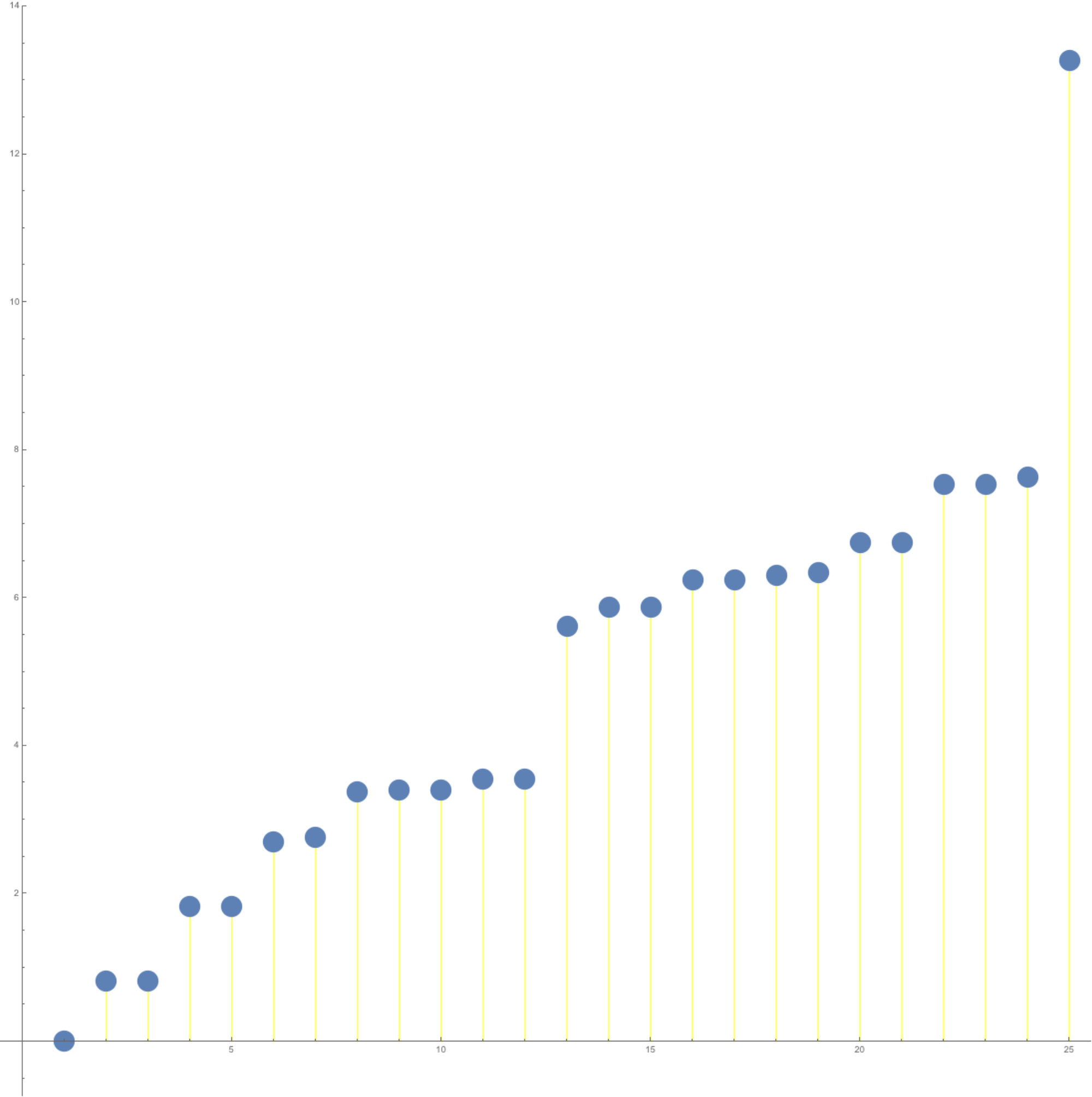
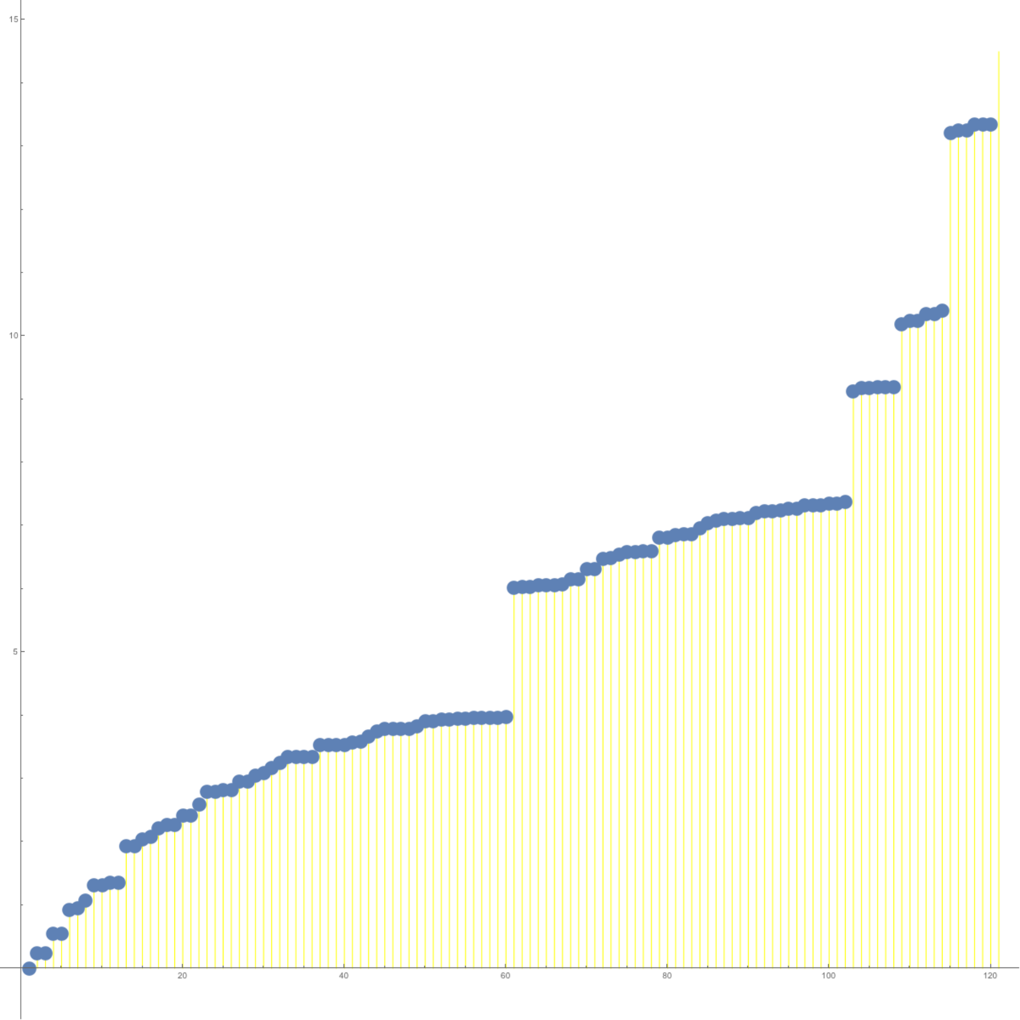
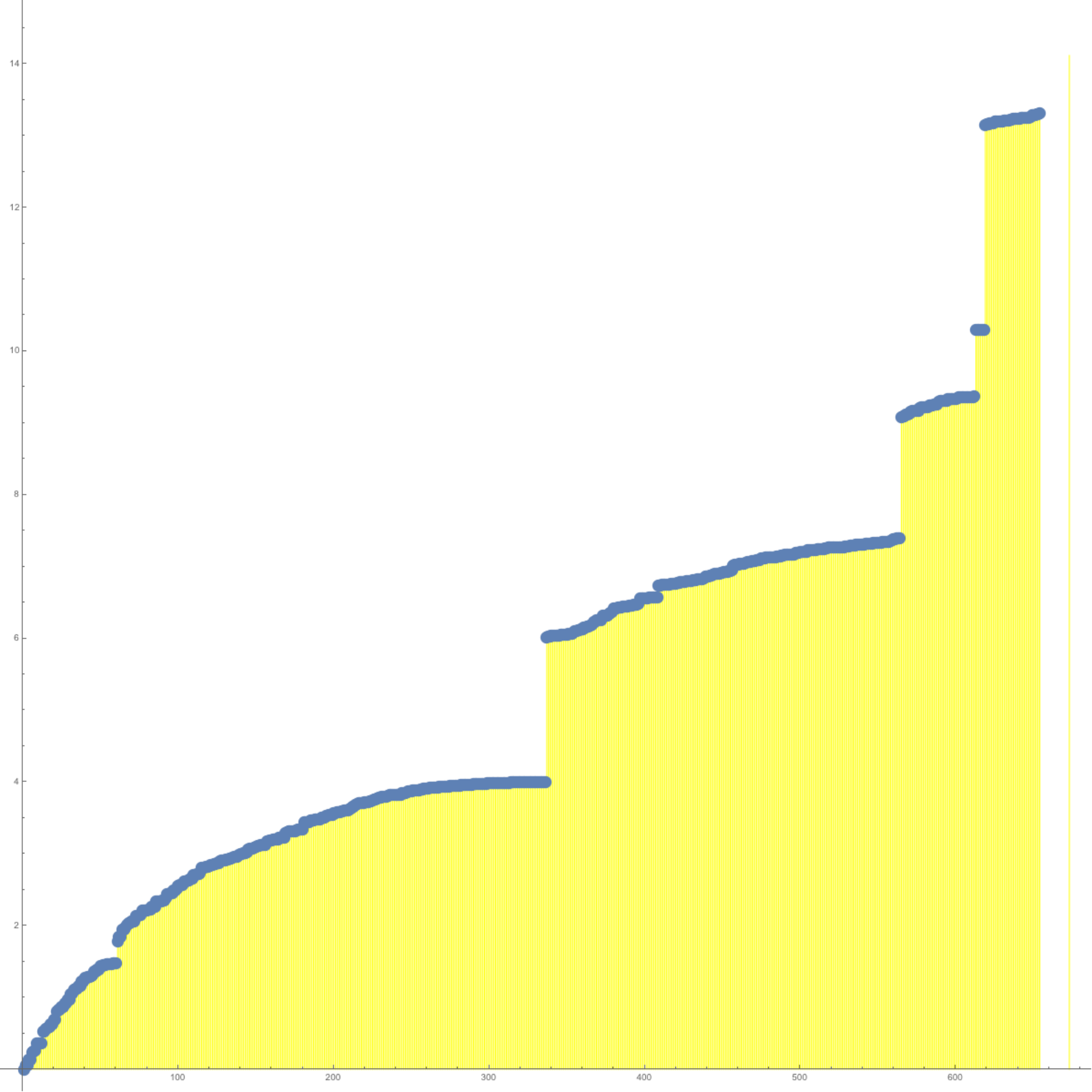
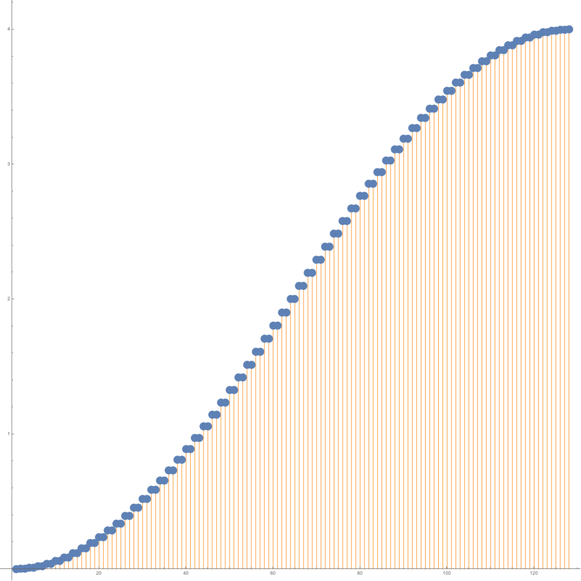
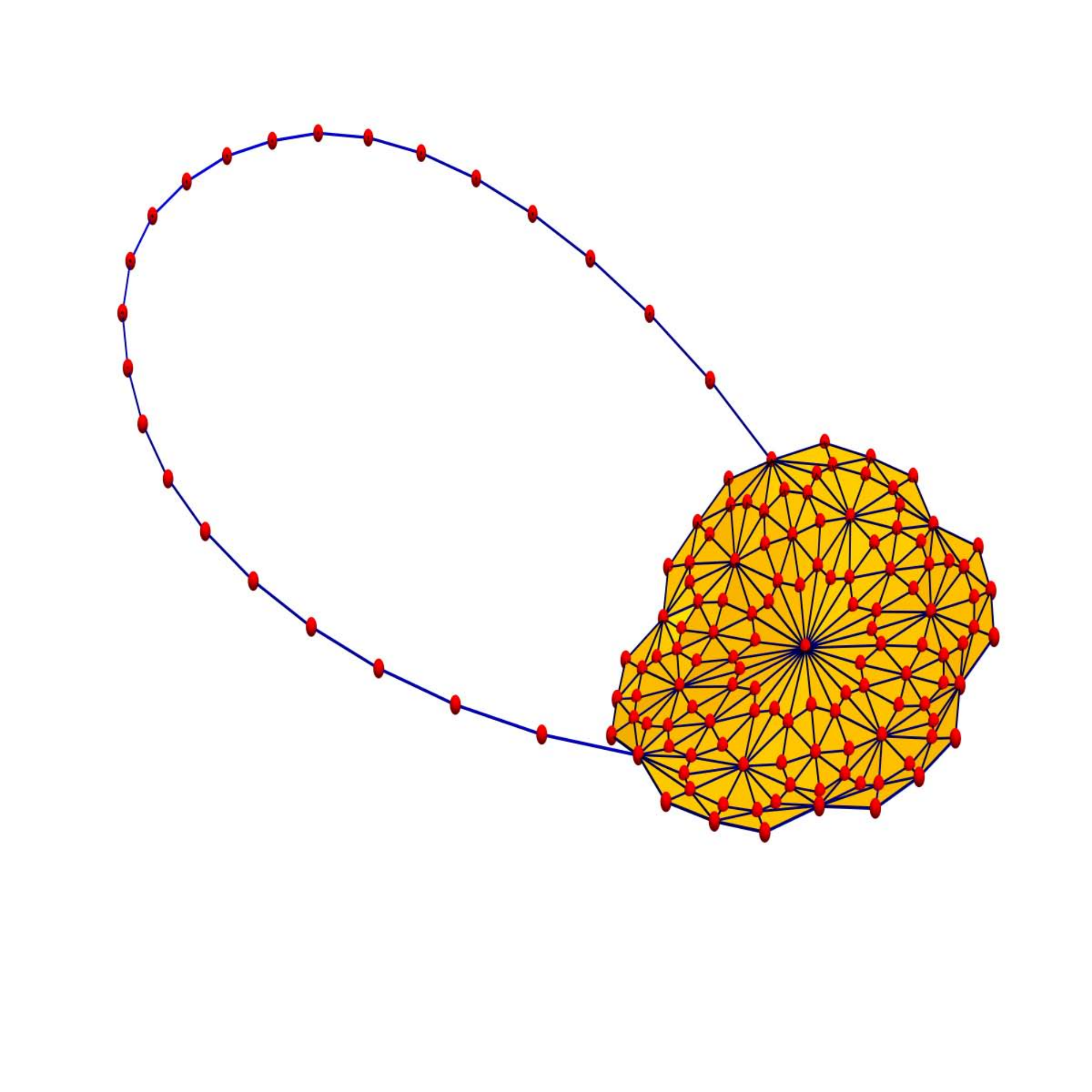
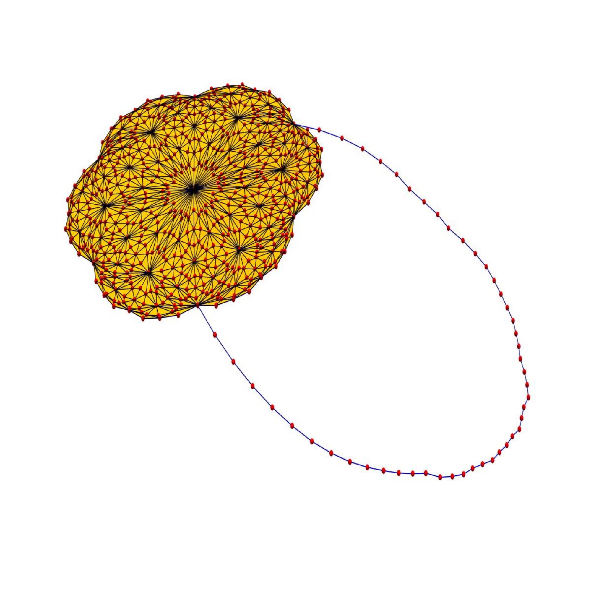
While experimenting with nodal surfaces for eigenfunctions of the Laplacian on discrete -spheres, where we expect the nodal surface of the ground state to be a -sphere in general, we also computed eigenvalues of refinements and got interested on how the eigenvalue distribution depends on refinements. While we expected some limit to be reached, we would have thought that the limit to depend on the topology of the initial graph. This is not the case. Starting with a -torus or a 2-sphere produces the same limiting function, as the figures illustrate and as we will show below. We can not push numerical experiments far, as the number of vertices of the refinements grows so fast. But the theory confirms this. The proof is rather elementary using a Lidskii lemma. Here is the main result:
Theorem 2 (Central limit of barycentric refinements).
The sequence converges in to a limiting distribution function which only depends on the dimension of the largest complete subgraph of .
The convergence is uniform on compact subsets in and exponentially fast in norm or in the norm for every compact interval . In the case , where we can compute the spectrum for circular graphs, we have an explicit limiting function . We first show that the limit exists for each graph and then prove that the limit is universal and only depends on the dimension of the largest complete subgraph of . The fact that a sequence of monotone functions in which converges in converges also uniformly on every closed interval with is known in real analysis (e.g. [38]). That the convergence can not be pushed to the boundary point follows from:
Lemma 3.
For , the function is not in , as the values grow exponentially with .
Proof.
The Courant-Fischer estimate (which is a special case of the Schur inquality in linear algebra) shows that , if is the number of vertices. Therefore, for every : then . Since the maximal degree increases indefinitely, the maximal eigenvalue grows, where is the number of vertices of . ∎
We do not know yet about the nature of the limiting functions in the case :
Problem: What is the spectral nature of the limiting density of states ? Does it have a discrete or singular part for ?
4. The one dimensional case
Proposition 4.
For , the limiting function is so that the limiting function is smooth.
Proof.
The eigenvalues of the Laplacian of circular graphs are explicitly known using discrete Fourier transform conjugating the Laplace operator on to the diagonal matrix with entries so that
By definition, we have . ∎
Proposition 5.
For , the Laplacian of the circular graphs satisfies the renormalization map , where is the quadratic map with Julia set and restricts the matrix to an invariant subspace of half the dimension.
Proof.
This is a direct verification for matrices. In the Fourier picture, it becomes a double angle formula of trigonometry. Algebraically, it is an identity for Jacobi matrices, the Laplacian of the free particle on the circular graph. For for example, we have the Laplacian
Now take the Laplacian of and form . This gives
We see that that there are two -dimensional subspaces of on which is isomorphic to the old operator . In the above notation, we have expressed this as . ∎
Remark: The quadratic map is associated to the Julia set of the map which is the ”tip of the tail” parameter in the Mandelbrot set . The polynomial is conjugated to a Tschebychev polynomial, which by the way are the polynomials for which the Julia set is an interval [2]. Alternatively, in the context of interval maps, the map is conjugated to the Ulam map . The density of the eigenvalues follows the arcsin probability distribution supported on . It has with cumulative distribution function . The absolutely continuous measure is the natural equilibrium measure on the Julia set, the measure which maximizes metric entropy and equals it to topological entropy .
5. Convergence
Intuitively, universal convergence is a consequence of the fact that
every simplex in spans more simplices producing a self similar pattern.
Smaller dimensional parts and contributions from boundary get washed away as
the refinement progresses, as in dimension , there are exponentially more
points than in dimension . Also in higher dimensions, we expect this to be
a setup for a renormalization scheme, as the spectrum on part of the graph is
close to the spectrum of the entire graph and different regions grow in the same manner.
We can not write the limiting as a fixed point of a renormalization map yet. It can
not be ruled out yet that the scalar Laplacian of could be related with the form
Laplacian of . In two dimensions, where only -forms are Fermionic,
the spectrum of is determined by the spectrum of the scalar -forms and the
-forms.
The refinements become more and more self-similar, even so the degrees become larger and larger. We will see that the average eigenvalue converges for in such a way that decreases with an exponential rate depending only on the dimension of the largest complete subgraph.
Problem: Is there also in dimension a functional equation for which the limiting is a solution? Is there a relation with an equilibrium measure of a Julia set as in ?
When we look at convergence of in , the limiting graph density relating the number of edges with the number of vertices matters.
Lemma 6.
which is the average vertex degree of .
Proof.
The trace of the matrix is the sum of the eigenvalues. By the Euler handshaking lemma, it is twice the number of edges. The average eigenvalue is therefore
∎
In the case of a circular graph, we have . In the case of the triangle graph, we have
The fact that the average degree goes to follows of also from Gauss-Bonnet, as is the curvature for graphs without subgraphs. Since the Euler characteristic of the triangle is , the sum of the curvature has to converge to . More generally, we have:
Corollary 7.
In any dimension , the one has exponentially fast.
Proof.
Indeed, as the number of boundary simplices grows like and the number of interior simplices grows like , the convergence is of the order . ∎
Since the largest vertex degree grows exponentially in , we know . The Cheeger inequality for graphs allows to say something about the ground state energy, the smallest nonzero eigenvalue of the connected graph .
Corollary 8.
The ground state energy converge to exponentially fast for .
Proof.
In dimension , where we know the explicit spectrum and because the number of vertices grows exponentially. In general, it follows from the fact that the Cheeger number goes to zero exponentially fast. ∎
In order to compare eigenvalues, one could use a perturbation result of Weyl which tells that for selfadjoint matrices , the eigenvalues are sandwiched between and . Since we need not only the individual eigenvalues to converge but also need a -convergence, the following variant of the Lidskii’s theorem which was used already in [26] is better suited:
Lemma 9 (Lidskii).
For any two selfadjoint complex matrices with eigenvalues and , one has .
The reduction to the standard Lidksii theorem was told me by Yoram Last [37]:
Proof.
Denote with the eigenvalues of the selfadjoint matrix and let be the unitary matrix diagonalizing so that . We calculate
The claim follows now from Lidskii’s inequality (see [45]) ∎
Proposition 10.
For any and , there exists a limiting eigenvalue distribution .
Proof.
We proceed by induction. For , we have explicit eigenvalues. For , we make a refinement and divide it up into 6 pieces. Lidskii shows that the eigenvalues of consist of copies of the eigenvalues of plus a correction term which comes from lower dimensional interfaces and is much smaller. In words, . As converges, the sequence is a Cauchy sequence. Now, lets go to the case . We have and again have a Cauchy sequence showing that the limit exists in . In each dimension we get a limiting function as the lower dimensional interfaces between the similar chambers grow exponentially slower than the chambers themselves. ∎
Corollary 11.
There exists a limiting density of states which is a measure on .
Proof.
As are monotone, it defines a measure . Since the limiting eigenvalue distribution is monotone, it defines a measure . ∎
With pointwise convergence, we would have weak convergence of to .
But we don’t know that yet.
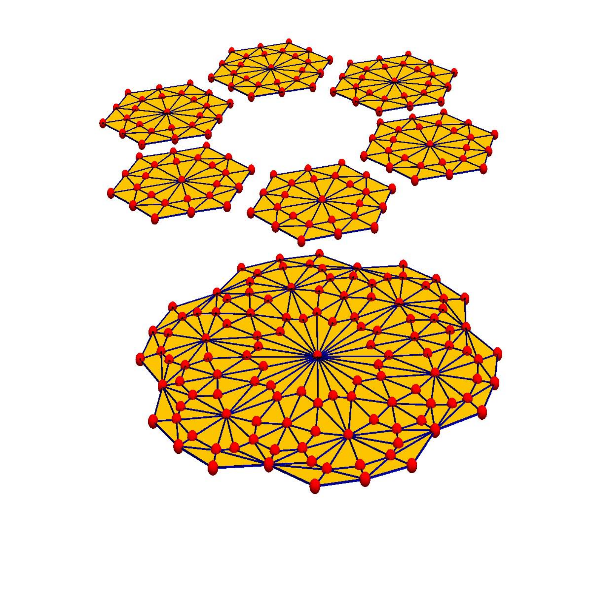
Lets now look at the proof of the theorem: we have to show that the limiting function does not depend
on the initial graph. Having seen convergence for a simplex , it follows for
a finite union of simplices glued along lower dimensional simplices. Each simplex
evolves in the same way under the barycentric evolution and the average is the same
function . When cutting the graph apart or disregarding lower dimensional parts,
the modifications lead to change on a set of vertices which becomes exponentially
less relevant as grows as it is lower dimensional.
This is justified by Lidskii’s estimate as we can estimate the sum of the eigenvalue differences.
6. Vertex degree distribution
Lets look at the vertex degree distribution . In the same way as for the spectrum, we can define a degree distribution function
The degree and eigenvalue distributions are linked by the Schur’s inequality so that one can deduce the following from the eigenvalues. It is also possible to do it directly:
Corollary 12 (Limiting vertex distribution).
There exists a limiting vertex distribution function . It is independent of the initial graph and depends only on the dimension of the largest complete subgraph of . The distribution satisfies for , .
Proof.
Splitting the graph into smaller graphs and noting that the
degrees of the lower dimensional walls can be neglected in the limit as the number
of vertices in those parts grows slower, we have a Cauchy sequence in .
An inequality of Schur
For any selfadjoint matrix , the Schur inequality
holds, where are the eigenvalues of and are the diagonal elements of . In the case we have equality since . The Schur inequality gives if the degrees of the graph and eigenvalues of the graph are ordered in an ascending way. ∎
Remark. A bit stronger than Schur is a result of Gone [1]) which assures that
if are the eigenvalues of the Laplacian
of and are the vertex degrees of
the graph . This implies that for each and suggest that
also in the limit for every .
In the case , the degree is related to the curvature
which adds up to the Euler characteristic of . We see that the curvature
distribution is related to the eigenvalue distribution.
In general we can look at the curvature
of a vertex which by Gauss-Bonnet-Chern [24]
adds up to the Euler characteristic of .
The limiting distribution works also for the Dirac operator and so for the Hodge Laplacian . The argument is the same.
Corollary 13.
For any , the Laplacian on -forms has a spectral limiting function which only depends on and the dimension of the largest simplex in .
In each dimension , the graph belonging to a simplex
can be cut (using some modifications on smaller dimensional sub graphs)
into smaller isomorphic pieces, which are of the form
. The -dimensional cuts do not matter in the limit as the
number of simplices in them grows exponentially less fast.

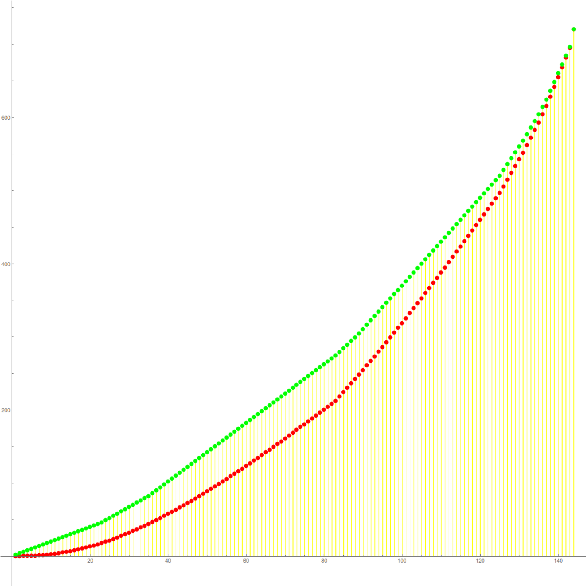
Since the matrices and have the same size, we compared
the distribution of the Hodge Laplacian on the level with the distribution of
the scalar Laplacian on the level and they appear comparable.
Because of super symmetry, the 1-form Laplacian has the same spectrum
than the union of the and -form Laplacians. The -form Laplacian is
related to the Laplacian of the dual graph.
There might be more relations if things are extended to Schrödinger operators. In [22], we looked at renormalization maps satisfying , where is a Laplacian on a barycentric refined circular graph. Its not clear whether there are algebraic relations for . For a triangle with Laplacian the Laplacian of the refinement and the form Laplacian have the same size
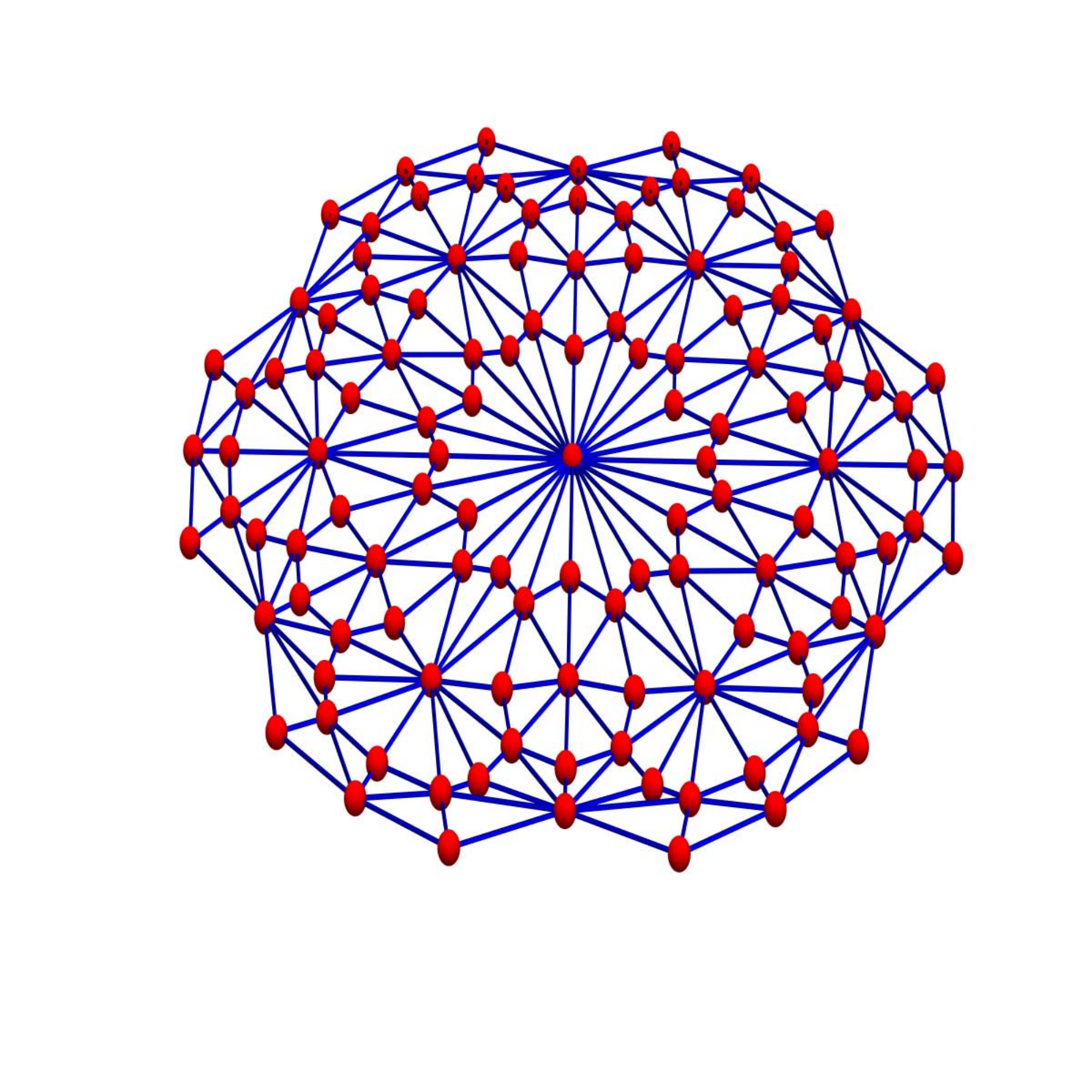
7. Figures


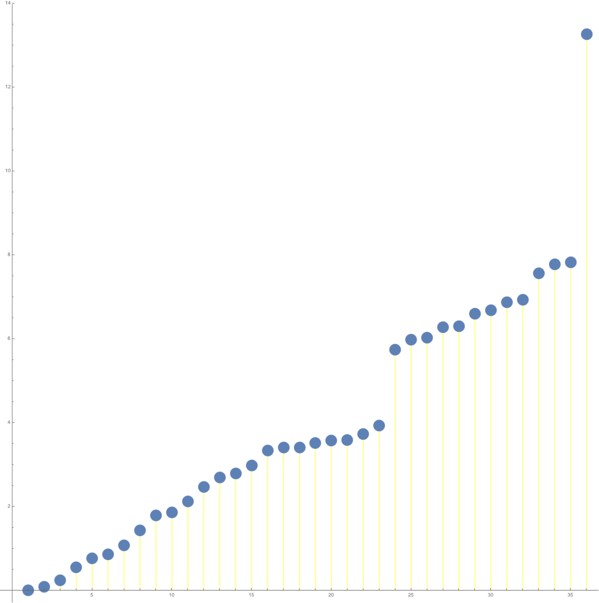
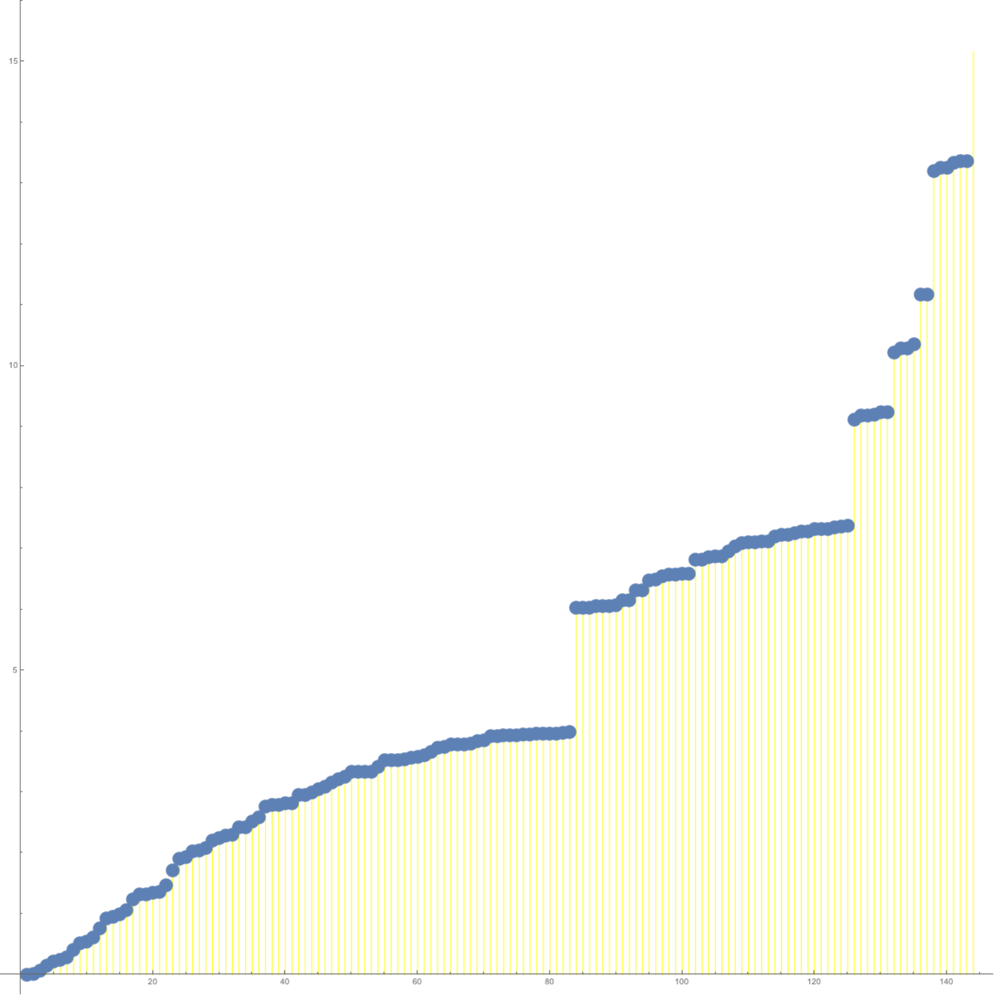
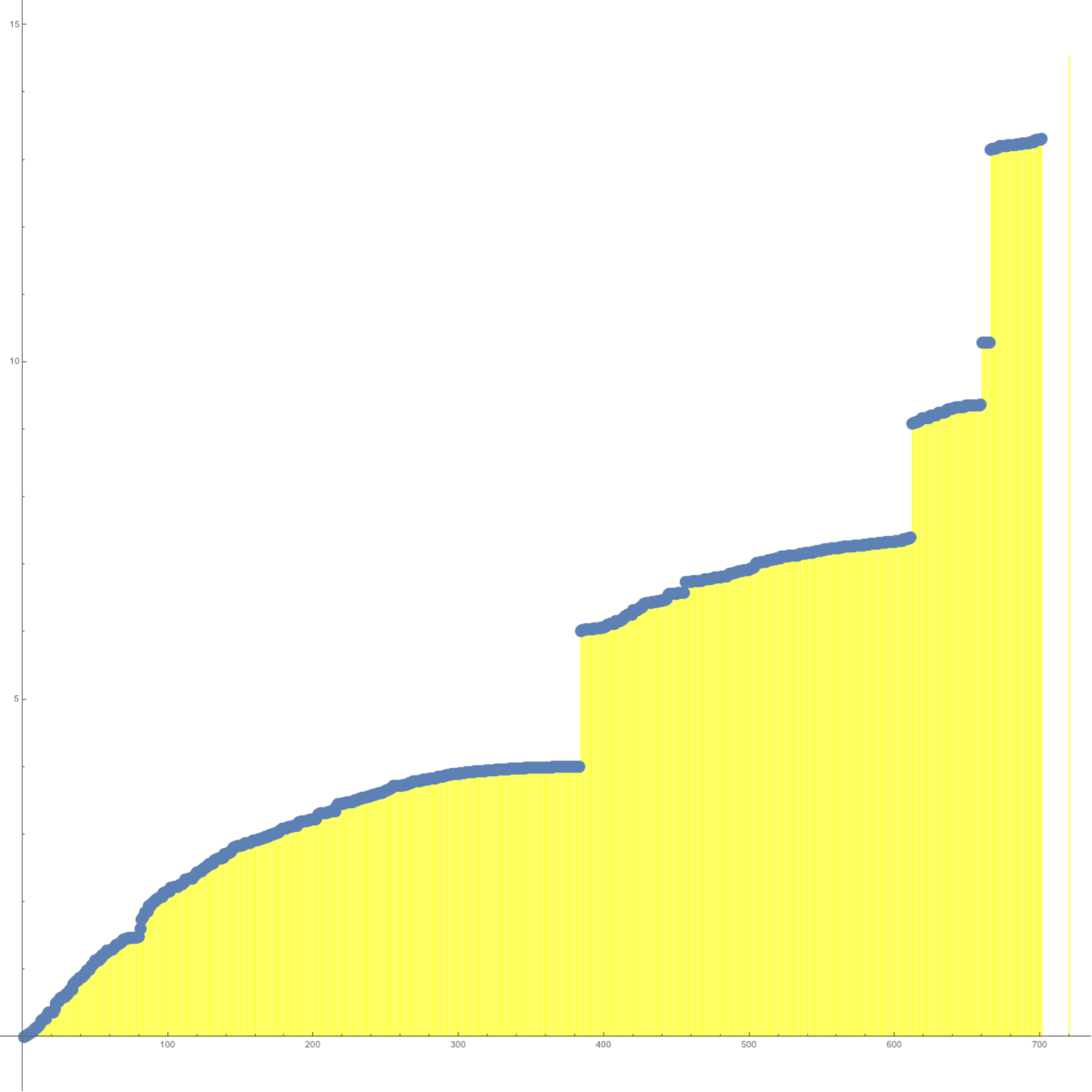

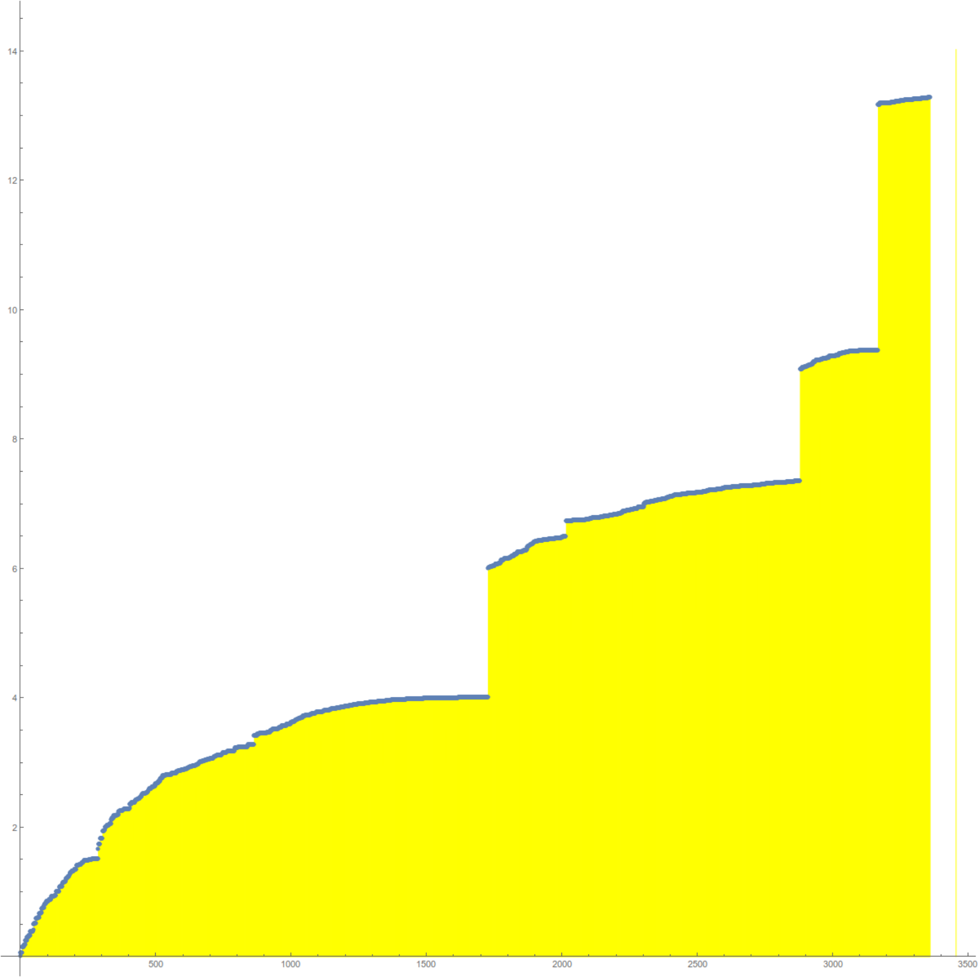


References
- [1] W.H. Haemers A.E. Brouwer. Spectra of graphs. Springer, 2010.
- [2] A. Beardon. Iteration of rational functions. Graduate Texts in Mathematics. Springer-Verlag, New York, 1990.
- [3] M. Berger. A Panoramic View of Riemannian Geometry. Springer Verlag, Berlin, 2003.
- [4] I. Chavel. Eigenvalues in Riemannian Geometry. Pure and applied mathematics. Academic Press Inc., Orlando, 1984.
- [5] B. Chen, S-T. Yau, and Y-N. Yeh. Graph homotopy and Graham homotopy. Discrete Math., 241(1-3):153–170, 2001. Selected papers in honor of Helge Tverberg.
- [6] F. Chung. Spectral graph theory, volume 92 of CBMS Regional Conf. Series. AMS, 1997.
- [7] Y.Colin de Verdière. Spectres de graphes. 1998.
- [8] P. Diaconis and L. Miclo. On barycentric subdivision. Combin. Probab. Comput., 20(2):213–237, 2011.
- [9] A.V. Evako. Dimension on discrete spaces. Internat. J. Theoret. Phys., 33(7):1553–1568, 1994.
- [10] A.V. Evako. The Jordan-Brouwer theorem for the digital normal n-space space . http://arxiv.org/abs/1302.5342, 2013.
- [11] M. Fiedler. A property of eigenvectors of nonnegative symmetric matrices and its application to graph theory. Czechoslovak Mathematical Journal, 25:619–633, 1975.
- [12] R. Forman. A discrete Morse theory for cell complexes. In Geometry, topology, and physics, Conf. Proc. Lecture Notes Geom. Topology, IV, pages 112–125. Int. Press, Cambridge, MA, 1995.
- [13] R. Forman. Combinatorial differential topology and geometry. New Perspectives in Geometric Combinatorics, 38, 1999.
- [14] G.A.Baker, D.Bessis, and P.Moussa. A family of almost periodic Schrödinger operators. Physica A, 124:61–78, 1984.
- [15] B. Hough. Tessellation of a triangle by repeated barycentric subdivision. Electron. Commun. Probab., 14:270–277, 2009.
- [16] A. Ivashchenko. Contractible transformations do not change the homology groups of graphs. Discrete Math., 126(1-3):159–170, 1994.
- [17] A.V. Ivashchenko. Graphs of spheres and tori. Discrete Math., 128(1-3):247–255, 1994.
- [18]
F. Josellis and O. Knill.
A Lusternik-Schnirelmann theorem for graphs.
http://arxiv.org/abs/1211.0750, 2012. - [19] O. Knill. Factorisation of random Jacobi operators and Bäcklund transformations. Communications in Mathematical Physics, 151:589–605, 1993.
- [20] O. Knill. Isospectral deformations of random Jacobi operators. Communications in Mathematical Physics, 151:403–426, 1993.
- [21] O. Knill. Isospectral deformation of discrete random Laplacians. In M.Fannes et al., editor, On Three Levels, pages 321–330. Plenum Press, New York, 1994.
- [22] O. Knill. Renormalization of of random Jacobi operators. Communications in Mathematical Physics, 164:195–215, 1995.
- [23]
O. Knill.
The dimension and Euler characteristic of random graphs.
http://arxiv.org/abs/1112.5749, 2011. - [24]
O. Knill.
A graph theoretical Gauss-Bonnet-Chern theorem.
http://arxiv.org/abs/1111.5395, 2011. - [25] O. Knill. A discrete Gauss-Bonnet type theorem. Elemente der Mathematik, 67:1–17, 2012.
- [26]
O. Knill.
The McKean-Singer Formula in Graph Theory.
http://arxiv.org/abs/1301.1408, 2012. - [27] O. Knill. A Brouwer fixed point theorem for graph endomorphisms. Fixed Point Theory and Applications, 85, 2013.
- [28]
O. Knill.
The Dirac operator of a graph.
http://http://arxiv.org/abs/1306.2166, 2013. - [29]
O. Knill.
An integrable evolution equation in geometry.
http://arxiv.org/abs/1306.0060, 2013. - [30]
O. Knill.
Isospectral deformations of the dirac operator.
http://arxiv.org/abs/1306.5597, 2013. - [31] O. Knill. Coloring graphs using topology. http://arxiv.org/abs/1410.3173, 2014.
- [32]
O. Knill.
A notion of graph homeomorphism.
http://arxiv.org/abs/1401.2819, 2014. - [33] O. Knill. Graphs with Eulerian unit spheres. http://arxiv.org/abs/1501.03116, 2015.
- [34]
O. Knill.
The Jordan-Brouwer theorem for graphs.
http://arxiv.org/abs/1506.06440, 2015. - [35] O. Knill. The Kuenneth formula for graphs. http://arxiv.org/abs/1505.07518, 2015.
- [36]
O. Knill.
The zeta function for circular graphs.
http://arxiv.org/abs/1312.4239, December 2013. - [37] Y. Last. Personal communication. 1995.
- [38] J.T. Lewis and O. Shisha. Lp convergence of monotone functions and their uniform convergence. Journal of Approximation Theory, 14:281–284, 1975.
- [39] T. Mantuano. Discretization of Riemannian manifolds applied to the Hodge Laplacian. Amer. J. Math., 130(6):1477–1508, 2008.
- [40] H.P. McKean and I.M. Singer. Curvature and the eigenvalues of the Laplacian. J. Differential Geometry, 1(1):43–69, 1967.
- [41] M.F.Barnsley, J.S.Geronimo, and A.N. Harrington. Almost periodic jacobi matrices associated with julia sets for polynomials. Commun. Math. Phys., 99:303–317, 1985.
- [42] O. Post. Spectral Analysis on Graph like Spaces, volume 2039 of Lecture notes in Mathematics. 2012.
- [43] P.VanMieghem. Graph Spectra for complex networks. Cambridge University Press, 2011.
- [44] S. Rosenberg. The Laplacian on a Riemannian Manifold, volume 31 of London Mathematical Society, Student Texts. Cambridge University Press, 1997.
- [45] B. Simon. Trace Ideals and Their Applications. AMS, 2. edition, 2010.
- [46] D.F. Snyder. Combinatorics of barycentric subdivision and characters of simplicial two-complexes. Amer. Math. Monthly, 113(9):822–826, 2006.
- [47] J. Leydold T. Bijikoglu and P. Stadler. Laplacian Eigenvectors of Graphs, volume 1915 of Lecture Notes in Mathematics. Springer, 2007.
- [48] J.H.C. Whitehead. Simplicial spaces, nuclei and m-groups. Proc. London Math. Soc., 45(1):243–327, 1939.