Leptoquark induced rare decay amplitudes $h\to\tau^{\mp}\mu^{\pm}$ and $\tau\to\mu\gamma$

The newly discovered Higgs boson $h$ at the mass 125 GeV is consistent with the Higgs boson predicted in the standard model (SM) [1]. The narrow decay width of a predicted size about 4 MeV in SM provides hope that the unusual rare decay due to new physics (NP) can have a measurable branching fraction. Recently, the CMS collaboration has reported [2] a possible excess in the decay process $h\to\tau^{\mp}\mu^{\pm}$ with a significance of 2.4 $\sigma$ in the search for the lepton flavor violation (LFV). Assuming SM Higgs production, CMS obtained the best fit for the branching fraction summed over $\tau^{-}\mu^{+}$ and $\tau^{+}\mu^{-}$,

We understand that it is too early to draw a positive inference until future analyses of higher statistics from both CMS and ATLAS experiments are performed. However, the present sensitivity at the $1\%$ level is interesting enough to call for possible NP to deliver such a detectable rate but satisfy other rare decay constraints such as $\tau\to\mu\gamma$,

at low energy. Indeed, there are a lot of theoretical activities[4, 5, 6, 7, 8, 9, 10, 11, 12, 13, 14, 15, 16, 17, 18, 19, 20, 21, 22] along this line of investigation. There were also a number of studies on LFV Higgs boson decays in literature [23]. We are particularly motivated by the leptoquark (LQ) associated with the third generation, which provides a large top quark mass insertion in the loop diagram. However, the LQ interactions also give rise to amplitudes for $\tau\to\mu\gamma$. We notice that the cancellation between two types of LQ contributions is possible for $\tau\to\mu\gamma$, leaving a large detectable decay rate for $h\to\tau^{\mp}\mu^{\pm}$. Each of these two types of LQs has been outlined in the literature, such as in Ref.[4], but the combined version necessary for the cancellation was overlooked.

The organization of the work is as follows. In the next section, we describe the LQ interactions associated with the top quark and tau lepton. In Sec. III and IV, we calculate the decay $\tau\to\mu\gamma$ and $h\to\tau^{\mp}\mu^{\pm}$, respectively. We give details on numerical results in Sec. V. We conclude in Sec. VI.

We associate the new LQs with the top quark of the third generation in order to avoid the very stringent constraints upon the flavor non-conservation among the first two generations. On the other hand, the mass insertion of the top quark can enhance the rate of the rare LFV Higgs decay mode among the second and the third generation leptons. To satisfy the electroweak gauge symmetry, we can classify two types of LQs, the first one $\chi^{{\hbox{$1\over 3$}}}$ is a weak $SU(2)$ singlet, and the other one $SU(2)$ doublet, i.e. $\Omega^{T}=(\Omega^{{\hbox{$5\over 3$}}},\Omega^{{\hbox{$2\over 3$}}})$. The superscript denotes the electromagnetic charge number. LQs transform under the $SU(3)$ color group as $\bf 3$ just like quarks. The relevant interactions are given by

The Feynman diagrams (for $\tau\to\mu\gamma$) that involve these LQ interactions are shown in Fig. 1. The shown $\epsilon$ symbol, basically $i\sigma_{2}$, links two $SU(2)$ doublets into a gauge invariant singlet. For brevity, we do not show other Levi-Civita symbols that contract Weyl spinor indexes. Also, $(Q_{3})_{L}^{T}=(t_{L},b_{L})$, $L_{\tau,L}=(\nu_{\tau,L},\tau_{L})^{T}$. The terms from exchanging $\tau\leftrightarrow\mu$ are needed to induce the LFV between the muon and the tau.

We start with the contributions from the singlet $\chi$. We define $t^{c}$ to be the charge conjugated state of $t$. In this way, we can avoid the use of the unfamiliar Feynman rule for two fermions flowing into a vertex. Instead, one fermion flows in and the other out. For example, the incoming $\tau$ enters the first vertex and turns into a departing $t^{c}$ plus a boson $\chi^{-{1\over 3}}$. The relevant vertices for the process $\tau\to\mu\gamma$ are

For the outgoing left-handed muon, the Feynman amplitude that the external photon line attaches to the $t^{c}$ line is given by

where $R$ stands for the right-handed chiral projection operator $(1+\gamma^{5})/2$. It is understood that the external spinors $\overline{u(\mu)}$ and $u(\tau)$ sandwich the Dirac chain. We keep track of the color factor 3 by a subscript $c$. Another amplitude where the photon attaches to $\chi^{-{1\over 3}}$ is

We set charges $q_{t^{c}}=-{\hbox{$2\over 3$}}$ and $q_{\chi^{-{1\over 3}}}=-{\hbox{$1\over 3$}}$. Using $z\leftrightarrow(1-z)$ in ${\cal M}_{1}$, we obtain

The numerator of the integral becomes $z^{2}-{\hbox{$z\over 3$}}$. The overall result is

So the amplitude is related to the integral function,

Our result is different from that in Ref.[4]. Note that there is another chiral amplitude for the outgoing right-handed muon, using $g_{L}^{\tau}g_{R}^{\mu}$. These two amplitudes do not interfere in the zero muon mass limit.

Now we switch to the contributions from the LQ doublet $\Omega$. The relevant vertices for the process $\tau\to\mu\gamma$ are

For the outgoing left-handed muon,

This corresponds to the diagram that the external photon line attaches to the $t$ line. Another amplitude where the photon attaches to $\Omega^{-{5\over 3}}$ is

We set charges $q_{t}={\hbox{$2\over 3$}}$ and $q_{\Omega^{-{5\over 3}}}=-{\hbox{$5\over 3$}}$. Using $z\leftrightarrow(1-z)$ in ${\cal M}_{1}$, we obtain

The numerator of the integral becomes $z^{2}-{\hbox{$5z\over 3$}}$. The overall result is

So the amplitude is related to the integral function,

Note that there is another chiral amplitude for the outgoing right-handed muon, using ${g^{\prime}}_{L}^{\tau}{g^{\prime}}_{R}^{\mu}$.

In general, the low energy effective operators of dim 5 are

The partial decay width of the process $\tau\to\mu\gamma$ is

The general loop formulas for the radiative transitions can be found in Ref.[24]

For the rare decay $h\to\tau\mu$, we start with the contribution from the $SU(2)$ singlet leptoquark $\chi^{-{\hbox{$1\over 3$}}}$ to the chiral amplitude of the outgoing right-handed $\tau$. We take the zero mass limit for $\mu$ and $\tau$. At the one loop level, the Higgs coupling to $\tau(p_{1})\bar{\mu}(p_{2})$ is induced via a triangle diagram, which involves internal $t^{c},\chi$ lines. First, we concentrate at the diagram that the external Higgs touches the internal $t^{c}$ line, as shown in Fig. 2.

We use the Feynman parameterization trick to carry over the integration. The parameters $\alpha,\beta,\gamma$ are assigned to the denominator factors $(\ell+p_{1})^{2}-m_{t}^{2}$, $(\ell-p_{2})^{2}-m_{t}^{2}$, $\ell^{2}-m_{\chi}^{2}$ respectively, under the constraint $\alpha+\beta+\gamma=1$. Then we complete the square of the denominator as follows,

Shifting the loop momentum, we simplify the numerator of the the Dirac matrices with the equation of motion,

Here the $s$ variable is simply $2p_{1}\cdot p_{2}=m_{h}^{2}$. The amplitude becomes

The domain $\tt L\!\!\backslash$ covers positive $\alpha$ and $\beta$, as well as $\alpha+\beta\leq 1$.

We perform the Wick’s rotation by Euclideanizing $\ell^{\prime 0}\to iq_{E4}$, $\ell^{\prime 2}\to-q_{E}^{2}$, $d^{4}\ell^{\prime}\to id^{4}q_{E}$, $d^{4}q_{E}\to d^{3}{\mbox{\boldmath{$q$}}}_{E}dq_{E4}=4\pi|{\mbox{\boldmath{$q$}}}_{E}|^{2}d|{\mbox{\boldmath{$q$}}}_{E}|dq_{E4}\to 4\pi(q_{E}^{2}\cos^{2}\phi){\hbox{$1\over 2$}}dq_{E}^{2}d\phi\to\pi^{2}q_{E}^{2}dq_{E}^{2}$. So

The logarithmic divergence has to be canceled by the one-particle reducible (1PR) diagrams with bubbles in the external lepton lines. The $h$ line is either attached directly to $\tau$ or $\mu$, picking up respectively the mass couplings $m_{\tau}$ or $m_{\mu}$, which are canceled by the propagators. It can be shown the corresponding 1PR contribution to be

Overall, $\log\Lambda^{2}$ terms cancel. Therefore the combined amplitude is

Note that in the intermediate step, we can choose an arbitrary $\Lambda$ for the convenience of the calculation.

Alternatively, one can use the Passarino-Veltman[25] (PV) functions. The integral before the Feynman’s parameterization as given in (21) is

The first term simply gives the triangle function

The second term after shifting the loop momentum gives the bubble function

The result including the 1PR bubbles is

We have cross-checked numerically that the $G$ value from PV functions and from the Feynman parameterization method match each other.

For the Feynman diagram that the Higgs touches the leptoquark, the required vertex originates from the bosonic interaction of $-\lambda_{\chi}H^{\dagger}H\chi^{\dagger}\chi$. The $G$ coefficient is updated with the new addition,

When we come to the contribution from the $SU(2)$ doublet leptoquark $\Omega$, it is easy to see the simple translation,

Here $m_{\Omega}$ is the mass of the $5\over 3$ charged leptoquark. More explicitly,

The partial decay width, summing both processes $h\to\tau^{\mp}\mu^{\pm}$, is

To suppress the highly constrained $\tau\to\mu\gamma$, we tune the cancellation

We choose a simplified scenario that only one chiral mode of the muon interactions is important. Say, $g_{L}^{\mu}\gg g_{R}^{\mu}$ and ${g^{\prime}}_{L}^{\mu}\gg{g^{\prime}}_{R}^{\mu}$, then we only finely tune the corresponding one constraint, i.e. the first of the two. The ratio of the couplings $g_{R}^{\tau}g_{L}^{\mu}/({g^{\prime}}_{R}^{\tau}{g^{\prime}}_{L}^{\mu})$ is given in Fig. 3 for the tuned cancellation in $\tau\to\mu\gamma$. The contour plot demonstrates that a large parameter space remains available for the required fine-tuning.

Figure 4 shows the predicted numerical size of Br($h\to\tau^{\mp}\mu^{\pm}$ both) versus $g_{R}^{\tau}g_{L}^{\mu}$ for various LQ masses when the tuned cancellation is satisfied. We have set $\lambda_{\chi,\Omega}=0$ in our numerical study. A desirable branching fraction at 1% level occurs for the coupling product $g_{R}^{\tau}g_{L}^{\mu}\simeq 0.3-1$ for the cases that $m_{\Omega}=m_{\chi}$ from 600 GeV to 1 TeV.

If we switch off either one of the canceling amplitudes in $\tau\to\mu\gamma$, the individual contribution to the Br($\tau\to\mu\gamma)$ is shown in Fig. 5. This demonstrates how much fine-tuning is required. The Br($\tau\to\mu\gamma)$ would be at about the 1 % level for 500 GeV LQ and $g_{R}^{\tau}g_{L}^{\mu}$ about 0.3 to 0.8 if only using one of the two canceling amplitudes. To go down from $10^{-2}$ to $10^{-8}$ in the branching ratio, the two amplitudes are required to cancel each other by almost one part in $10^{3}$.

Reference [4] also proposed a mechanism of cancellation in the amplitude of $\tau\to\mu\gamma$ with the help of an additional vectorial top-like quark. However, the detailed gauge quantum numbers of the added structure have not been shown to be feasible.

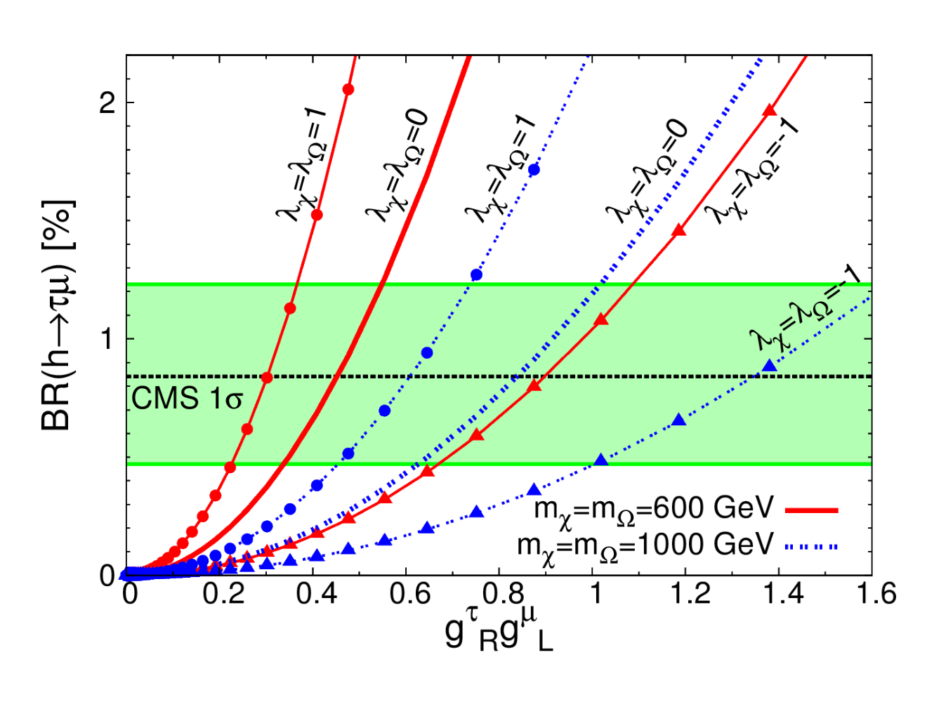
So far, we have set $\lambda_{\chi,\Omega}=0$. We show in Fig. 6 the branching ratio Br$(h\to\tau^{\mp}\mu^{\pm})$ for various choices of $\lambda_{\chi}=\lambda_{\Omega}=-1,0,1$. The tuned cancellation of Eq. (35) is satisfied. It gives additional freedom to achieve the desirable branching ratio for the rare Higgs decay.

The rare decay of $h\to\tau^{\mp}\mu^{\pm}$ can be at the current reachable sensitivity through the LFV LQ interactions, however fine-tuning is needed to avoid the stringent constraint from the null observation of $\tau\to\mu\gamma$. Here we have invoked more than one LQs, which couple to the third generation quarks, and the second and third generation leptons, in order to achieve a cancellation in $\tau\to\mu\gamma$ but sizable contributions to $h\to\tau^{\mp}\mu^{\pm}$.

There is another issue related to possible contributions of these LQs to the muon anomalous magnetic moments (aka $g-2$). It was shown a long time ago [26] and more recently [27] that if we choose, as we have chosen in the above analysis, the left-handed coupling to be much larger than the right-handed coupling for the muon, i.e. $g_{L}^{\mu}\gg g_{R}^{\mu}$ and ${g^{\prime}}_{L}^{\mu}\gg{g^{\prime}}_{R}^{\mu}$, the LQ contribution to $g-2$ is highly suppressed by $m_{\mu}/M_{LQ}$ and very small for the LQ mass range that we considered in this work.

The required leptoquarks $\chi$ and $\Omega$ can be strongly produced at the high energy and high luminosity hadron colliders. They have dominant decay channels into the top quark and the charged lepton $\tau$ or $\mu$. That is a very identifiable signature. Both ATLAS [29] and CMS [28, 30] collaborations have searched for the third generation leptoquarks via pair production by strong interaction. The CMS have searched for the third generation LQ with electric charged $-1/3$ (similar to the $\chi^{-1/3}$ of this work) decaying to a top quark and a tau lepton. They put a limit of 685 GeV at 95% CL on $m_{\chi}$ [28]. On the other hand, both ATLAS [29] and CMS [30] searched for the third generation LQ with electric charge $-2/3$ decaying into a $\bar{b}$ antiquark and a tau lepton (similar to $\Omega^{-2/3}$ in this work), and put a limit of 534 and 740 GeV, respectively.

Therefore, there are still plenty of mass ranges for $\chi^{-1/3}$ beyond 685 GeV and for $\Omega^{-2/3,-5/3}$ beyond 740 GeV that one can directly search for a top or bottom quark with a tau or muon at the Run 2 of LHC-13.

We thank N. Kosnik (on behalf of authors of Ref.[4]) for the communication about the external wave function renomalization in the process $h\to\tau\mu$. W.-Y. K. thanks the National Center of Theoretical Sciences and Academia Sinica, Taiwan, R.O.C. for hospitality. This research was supported in parts by the Ministry of Science and Technology (MOST) of Taiwan under Grant Nos. 102-2112-M-007-015-MY3 and by US DOE under Grant No. DE-FG-02-12ER41811.

References

• [1] See for example, K. Cheung, J. S. Lee and P. Y. Tseng, Phys. Rev. D 90, 095009 (2014) [arXiv:1407.8236 [hep-ph]].
• [2] V. Khachatryan et al. [CMS Collaboration], arXiv:1502.07400 [hep-ex].
• [3] B. Aubert et al. [BaBar Collaboration], Phys. Rev. Lett. 104, 021802 (2010) [arXiv:0908.2381 [hep-ex]].
• [4] I. Dorsner, S. Fajfer, A. Greljo, J. F. Kamenik, N. Kosnik and I. Nisandzic, JHEP 1506, 108 (2015) [arXiv:1502.07784 [hep-ph]].
• [5] R. Harnik, J. Kopp and J. Zupan, JHEP 1303, 026 (2013) [arXiv:1209.1397 [hep-ph]].
• [6] M. D. Campos, A. E. C. Hernández, H. Päs and E. Schumacher, Phys. Rev. D 91, no. 11, 116011 (2015) [arXiv:1408.1652 [hep-ph]].
• [7] A. Celis, V. Cirigliano and E. Passemar, arXiv:1409.4439 [hep-ph].
• [8] D. Aristizabal Sierra and A. Vicente, Phys. Rev. D 90, no. 11, 115004 (2014) [arXiv:1409.7690 [hep-ph]].
• [9] C. J. Lee and J. Tandean, JHEP 1504, 174 (2015) [arXiv:1410.6803 [hep-ph]].
• [10] J. Heeck, M. Holthausen, W. Rodejohann and Y. Shimizu, Nucl. Phys. B 896, 281 (2015) [arXiv:1412.3671 [hep-ph]].
• [11] A. Crivellin, G. D†¢Ambrosio and J. Heeck, Phys. Rev. Lett. 114, 151801 (2015) [arXiv:1501.00993 [hep-ph]].
• [12] L. de Lima, C. S. Machado, R. D. Matheus and L. A. F. do Prado, arXiv:1501.06923 [hep-ph].
• [13] I. de Medeiros Varzielas and G. Hiller, JHEP 1506, 072 (2015) [arXiv:1503.01084 [hep-ph]].
• [14] D. Das and A. Kundu, Phys. Rev. D 92, no. 1, 015009 (2015) [arXiv:1504.01125 [hep-ph]].
• [15] A. Crivellin, G. D†¢Ambrosio and J. Heeck, Phys. Rev. D 91, no. 7, 075006 (2015) [arXiv:1503.03477 [hep-ph]].
• [16] B. Bhattacherjee, S. Chakraborty and S. Mukherjee, arXiv:1505.02688 [hep-ph].
• [17] Y. n. Mao and S. h. Zhu, arXiv:1505.07668 [hep-ph].
• [18] B. Altunkaynak, W. S. Hou, C. Kao, M. Kohda and B. McCoy, arXiv:1506.00651 [hep-ph].
• [19] X. G. He, J. Tandean and Y. J. Zheng, arXiv:1507.02673 [hep-ph].
• [20] C. W. Chiang, H. Fukuda, M. Takeuchi and T. T. Yanagida, arXiv:1507.04354 [hep-ph].
• [21] W. Altmannshofer, S. Gori, A. L. Kagan, L. Silvestrini and J. Zupan, arXiv:1507.07927 [hep-ph].
• [22] A. Crivellin, J. Heeck and P. Stoffer, arXiv:1507.07567 [hep-ph].
• [23] A. Pilaftsis, Phys. Lett. B 285, 68 (1992); J. G. Korner, A. Pilaftsis and K. Schilcher, Phys. Rev. D 47, 1080 (1993) [hep-ph/9301289].
• [24] L. Lavoura, Eur. Phys. J. C 29, 191 (2003) [hep-ph/0302221].
• [25] G. Passarino and M. J. G. Veltman, Nucl. Phys. B 160, 151 (1979).
• [26] K. m. Cheung, Phys. Rev. D 64, 033001 (2001) [hep-ph/0102238].
• [27] F. S. Queiroz and W. Shepherd, Phys. Rev. D 89, no. 9, 095024 (2014) [arXiv:1403.2309 [hep-ph]].
• [28] V. Khachatryan et al. [CMS Collaboration], JHEP 1507, 042 (2015) [arXiv:1503.09049 [hep-ex]]/
• [29] G. Aad et al. [ATLAS Collaboration], JHEP 1306, 033 (2013) [arXiv:1303.0526 [hep-ex]].
• [30] V. Khachatryan et al. [CMS Collaboration], Phys. Lett. B 739, 229 (2014) [arXiv:1408.0806 [hep-ex]].