Light top squarks in lepton number model with a right handed neutrino and the LHC
Abstract
We investigate the phenomenology of top squarks at the Large Hadron Collider (LHC) in a supersymmetric model where lepton number is identified with an approximate symmetry in such a way that one of the left chiral sneutrinos can acquire a large vacuum expectation value () and can play the role of the down-type Higgs. This -symmetry allows a subset of trilinear -parity violating interactions, which determine the collider phenomenology of this model in a significant way. The gauginos are Dirac particles and gluinos are relatively heavy in this class of models. The model contains a right handed neutrino superfield, which gives a tree level mass to one of the active neutrinos. An order one neutrino Yukawa coupling also helps enhance the Higgs boson mass at the tree level and results in a very light bino-like neutralino () with mass around a few hundred MeV, which is a carrier of missing (transverse) energy (). The model can accommodate two rather light top squarks, compatible with the observed mass of the Higgs boson. The lighter top squark () can decay into , and thus the signal would be similar to the signal of top quark pair production at the LHC. In addition, fully visible decays such as can give rise to interesting final states. Such signals at the LHC combined with other features like a heavy gluino could provide a strong evidence for this kind of a model. Our analysis shows that GeV and TeV can be probed with 5 statistical significance at the 13 TeV LHC with 300 (3000) fb-1 of integrated luminosity. Finally, we observe that in the presence of super-light carriers of , the so-called ‘stealth’ top squark scenario may naturally appear in our model.
pacs
14.80.Ly, 12.60.Jv, 14.65.Ha, 11.30.PbI Introduction
The discovery of a Higgs boson at the Large Hadron Collider (LHC) with a mass around 125 GeV [1, 2] is of immense importance in high energy physics and, in particular, in the context of electroweak symmetry breaking. However, in spite of its enormous success over the years, the Standard Model (SM) of particle physics suffers from several drawbacks. From a theoretical perspective, the naturalness problem remains a troublesome issue in the framework of SM. Supersymmetry (SUSY) renders an elegant solution to this problem and has become the most popular choice for physics beyond the standard model (BSM) to date. Nevertheless, searches for superpartners by the LHC collaborations (ATLAS and CMS) in collisions at the centre-of-mass energies of TeV and 8 TeV have shown no significant excess [3, 4] over the SM background. This has put stringent lower limits on the superpartner masses in many different SUSY scenarios. Recent experimental analyses within the framework of a simplified phenomenological minimal supersymmetric standard model (pMSSM) have set a lower bound of 1.7 TeV [5] for comparable masses of the gluino and the first two generation squarks.
On top of that, finding a Higgs boson with a mass 125 GeV and the non-observation of any signals of physics beyond the SM have severely constrained many supersymmetric scenarios which are otherwise very well motivated. In view of this, models with Dirac gauginos and symmetry have become popular as they can significantly lower the current exclusion bounds on the first and second generation squarks and at the same time can address the 125 GeV Higgs boson even in the presence of lighter top squarks. Other virtues of such scenarios include significant suppression of flavor- as well as CP-violating effects. Assorted versions of models with Dirac gauginos and symmetry can be found in the literature [6, 7, 8, 9, 10, 12, 11, 13, 14, 15, 16, 17, 18, 19, 21, 20, 22, 23, 24, 25, 26, 27, 28, 29, 30, 31, 32, 33, 34, 36, 37, 38, 35, 49, 50, 39, 40, 41, 42, 43, 44, 45, 46, 47, 48, 51, 52, 53, 54, 55, 56, 57, 58, 59, 60, 61, 62, 63, 64, 65, 66, 67].
On the other hand, experiments in the neutrino sector have firmly established the fact that neutrinos have tiny masses and non-trivial mixings. Non-vanishing neutrino masses and mixings [68, 69, 70, 71] are very important indications of new physics. An interesting question to investigate is whether models with Dirac gauginos could also provide explanation for observed neutrino masses and mixings. As we shall describe later on, the introduction of a right-handed neutrino superfield with an appropriate -charge and Yukawa coupling ‘’ can give rise to a small neutrino mass of the right order at the tree level. At the same time, an order one ‘’ generates an additional tree level contribution to the Higgs boson mass. Thus, physics in the Higgs sector and the physics in the neutrino sector become intimately related in this model. This gives an opportunity to look into the Higgs sector through the neutrino-window and vice-versa. The additional tree level contribution to the Higgs boson mass also opens up the possibility of having rather light top squarks in the spectrum. This can also ameliorate the situation with so called ‘naturalness’ that is somewhat compromised in popular SUSY frameworks like the MSSM. There, the top squark masses are pushed to higher values ( (TeV)) to ensure a Higgs boson as heavy as observed at the LHC. Another very interesting outcome of this scenario is to have a very light bino-like neutralino, also identified as the lightest supersymmetric particle (LSP), with a mass in the range of a few hundred MeVs. The scenario violates -parity. Thus, such a light neutralino LSP could decay to SM fermions. However, the decay length turns out to be much larger than the collider dimension [72]. Hence it would essentially contribute to missing transverse energy (MET; ).
In such a backdrop, we study the phenomenology of light top squarks at the LHC in a symmetric model, first introduced in references [45, 46] and later on augmented by a right handed neutrino superfield in references [52, 58, 63]. The -charges are identified with the lepton numbers in such a way that the left chiral sneutrino can be large, and are not constrained by the Majorana mass of the neutrinos. Thus, the sneutrino can play the role of a down type Higgs field. There also exists a subset of -parity violating operators, mixings between the neutrinos and the neutralinos, as well as, between the charged leptons and the charginos. Once symmetry is invoked, the gauginos cease to have Majorana masses. However, they can acquire Dirac masses which requires additional chiral superfields living in the adjoint representation of the SM gauge group. It is somewhat crucial in the context of the present work to note that -symmetric models also prohibit the traditional trilinear scalar couplings ( terms) and the Higgsino mass parameter ( term). To generate a term, one needs to incorporate two more chiral superfields and with appropriate -charges.
The main motivation for having a right handed neutrino superfield is to have a tree level neutrino mass [52]. However, such a simple extension has enormous implication for the lightest CP even Higgs boson mass [52, 63] and for the dark matter sector [58].
The squarks in the present context carry a non-zero -charge () and hence a non-zero lepton number since lepton number is identified with the -charges. Top squarks can naturally be light in this model and can have novel signatures at the LHC. In the present work, we take the obviously natural direction of connecting to the top squark sector which is very much in the focus of the current LHC programme and thus could be put to test in a straight-forward way. This work presents for the first time the collider implications of the very characteristic top squark sector of the scenario under consideration. Various possibilities in the decays of both top squarks are discussed in detail. A novel final state in the form of is highlighted where the final state objects can, in principle, be reconstructed to the mass of the heavier top squark. The decay of the top squark to differs from typical -parity violating MSSM decay modes, and is typical for this model. This also provides us with an interesting handle, using which the reach of can be enhanced significantly, so much so, that the enhanced rate could also lead to its discovery even before its lighter cousin.
As for , pair production of top squarks and their subsequent decays might lead to signal similar to top quark pair production and provide important information on the model and, in particular, on the scenario with an order one neutrino Yukawa coupling ‘’. A characteristic difference in the signal is in the form of a somewhat softer , when compared to similar values in the MSSM. This is because of the presence of a MeV neutralino LSP, which is again a salient feature of our scenario. It is also demonstrated how various decay modes of remain simultaneously open thus necessitating a thorough analysis of the experimental data from the 13 TeV run of the LHC.
The paper is organised as follows. A brief description of the model is presented in section II. The neutral scalar sector of the model and its characteristic features are discussed in section III. Section IV describes the electroweak gauginos in general. We start with a generic discussion of the neutralino sector and its role in generating the tree level neutrino mass both in conserving case as well as taking into account mild violation of this -symmetry. We discuss the possibility of mixings among the neutralinos and the neutrinos. Later on, we discuss the chargino sector of this model and the corresponding mixing between the charginos and the electron. The focus area of this work, that is to say, the top squark sector is described in section V. Expressions for the decay rates in various relevant modes are presented. The latest bounds on the the masses of the top squarks as reported by the LHC collaborations are also discussed. The model is incorporated in SARAH (v4.4.1) [73, 74, 75]. In section VI we present a few benchmark points that reflect the characteristic decay patterns of the two top squarks and are found to be instrumental in shaping the interesting signatures at the LHC. Section VII is devoted to the actual simulation study of the signals and the most relevant backgrounds using event generators. Estimations of the reaches in the masses of the the top squarks are also presented. In section VIII we briefly analyse the issue of the ‘stealth’ top squark which arises naturally in our scenario. We summarise with some concluding remarks in section IX.
II The -lepton number model
We minimally extend an -symmetric model, first discussed in [45, 46], by a single right handed neutrino superfield [52]. Along with the chiral superfields of the minimal supersymmetric standard model (MSSM) superfields, , , , , , , , the model contains two ‘inert’ doublet superfields and with opposite hypercharges. To prohibit spontaneous -breaking and hence the emergence of -axions, the scalar components of and are barred from receiving any nonzero . This is why and are labeled as ‘inert’. Similarly, the scalar component of does not acquire any nonzero . The Dirac gaugino masses can be constructed with the introduction of chiral superfields, living in the adjoint representation of the SM gauge group. A singlet is needed to form a Dirac mass for the gaugino, a triplet under is required to have a Dirac mass for the gauginos and similarly an octet under must be there to generate the Dirac gluino mass. The charges of the chiral superfields along with their SM gauge quantum numbers are shown in table 1.
| Superfields | , , | |
|---|---|---|
| (3, 2, ) | 1 | |
| (, 1, ) | 1 | |
| (, 1, ) | 1 | |
| (, 2, ) | 0 | |
| (, 1, ) | 2 | |
| (, 2, ) | 0 | |
| (, 2, ) | 0 | |
| (, 2, ) | 2 | |
| (, 2, ) | 2 | |
| (, 1, ) | 0 | |
| (, 3, ) | 0 | |
| (, 1, ) | 0 | |
| (, 1, ) | 2 |
Note that the scalar components transform in the same manner as their respective chiral superfields whereas the fermions have -charge one less than that of the corresponding chiral superfields. Following reference [45], we also identify the lepton numbers of the component fields to the negative of their -charges. Such an identification leaves the lepton number assignments of the SM fermions unchanged from the usual ones while the superpartners acquire non-standard lepton numbers. As mentioned in the introduction, it is quite conspicuous that the left chiral sneutrino can be large since they do not become constrained by the lepton number violating Majorana neutrino masses [45]. As a result, the sneutrino can play the role of a down type Higgs field. It is now possible to integrate out the superfields and , which simplifies the superpotential and the scalar potential considerably. At this point all the three sneutrinos can acquire substantial s. However, without any loss of generality, one can always choose a basis in which only one of the sneutrinos get a non-zero , which we choose to be the electron type sneutrino11 1 It should be noted at this point that the formulation, though independent of this kind of a choice of a particular basis, could have crucial impacts on the actual observables at the experiments. We justify our choice later in this paragraph., whereas, the s of the other two sneutrino fields are zero. Thus, the electron sneutrino (, ) plays the role of a down type Higgs field. With this basis choice and the assumptions of [52, 63], the superpotential takes the following form;
| (1) | |||||
| (2) |
where is the up-type Yukawa coupling, is the Higgsino mass parameter consistent with the -charge assignments. ‘’ represents the neutrino Yukawa coupling, and are the trilinear couplings and finally is the coefficient of the bilinear term .
Note that, for simplicity in this work we have neglected the terms , , and from the superpotential. As long as , , , and -s of the scalar components of and are very small ( GeV, as we shall consider later), we do not expect any significant changes in the analysis and the results presented in this work.
The prime in indicates the mass basis for the down type quarks and charged leptons. When the electron sneutrino gets a , the first two terms in give masses to the down type charged leptons and quarks. However, invariance ensures that the operator cannot generate a mass for the electron. The electron mass can be generated from higher dimensional operators suppressed by a mass scale as discussed in [45]. Such operators would, in principle, contribute to the masses of other charged leptons as well. However, these contributions will be subdominant compared to the contribution to their masses from the operators. This makes it a natural choice for the electron sneutrino to acquire a non-zero . The other two terms in include all the trilinear -parity violating but lepton number preserving terms in this model.
In a realistic supersymmetric model, one needs to incorporate soft SUSY breaking terms such as the gaugino and the scalar mass terms. The Lagrangian consisting of the Dirac gaugino mass terms [45] can be written as
where is a spurion superfield parametrising -type SUSY breaking. ’s are the field strength tensors containing the gauginos of the MSSM vector superfields. The -term generates Dirac gaugino masses which can be schematically written as , where ’s are the order one coefficients and is the scale of SUSY mediation.
Similarly, -conserving but soft SUSY breaking terms in the scalar sector can be generated from a spurion superfield , where [45]. The non-zero of the -term generates the scalar soft terms. In the rotated basis where only the electron type sneutrino acquires a , the soft SUSY breaking terms are given by
| (4) | |||||
It is important to note that the scalar singlet tadpole term () is suppressed [42] in the scenarios with Dirac gaugino masses and that is what we will consider in the present context. With this short description of the theoretical framework we now proceed to describe the scalar and the fermionic sectors of the model in appropriate details.
III The neutral scalar sector and the Standard Model-like Higgs boson
In this section we discuss the CP-even scalar sector, followed by a rather important discussion on the lightest CP-even mass eigenstate. The scalar potential receives contributions from the -term, the -term, the soft-SUSY breaking terms and the dominant quartic terms generated at one loop and can be written down as
| (5) |
From the scalar potential and the subsequent minimization equations, one can now write down the CP-even scalar mass matrix in the basis , where the subscript indicates the real parts of the corresponding superfields. Both and carry -charges of two units and hence gets decoupled from the CP-even scalar mass matrix. In the -symmetric scenario the elements of CP-even scalar mass matrix are given by [52]
| (6) |
The ’s appearing only in and quantify the dominant one-loop radiative corrections22 2 See reference [22, 45] for a detailed discussion. to the quartic potential coming from the terms , and where
| (7) |
are the singlet and triplet soft masses while the singlet and the triplet s are denoted by and , respectively [22]. are the and gauge coupling constants, are the Dirac bino and wino masses, respectively. , where is the of the up-type neutral Higgs field and represents the of the electron type sneutrino. The ellipsis at the end of each expression stands for missing subdominant terms.
In this work, we study a simplified scenario in which the singlet and the triplet s are very small. These effectively decouple the corresponding scalar fields. Thus, the CP-even scalar mass-squared matrix turns out to be a one and can be written down in a compact form as
| (8) |
where and . As long as , where is the CP-odd Higgs mass, we find that the tree level upper bound on the lightest CP-even Higgs boson mass is [52]
| (9) |
Clearly, this result is very interesting since for a large neutrino Yukawa coupling, , the Higgs boson mass receives a large tree level enhancement. This additional tree level contribution grows at low and becomes significant for order one neutrino Yukawa coupling ‘’ [52, 63]. The resulting enhancement could play a significant role in lifting the Higgs boson mass to 125 GeV. Furthermore, this additional contribution ameliorates the ‘naturalness’ (pertaining to the mass of the Higgs boson) issue in the MSSM. However, this tree level contribution gets diluted at large values of . There, the one loop quartic corrections [22, 45] can come into play and can substantially enhance the Higgs boson mass in the presence of order one couplings, and , as shown in equation 7. Thus, even for larger values of , one can easily find a Higgs boson as heavy as observed at the LHC experiments, when the top squarks are relatively light.

Figure 1 illustrates the region in the plane of and compatible with 124.7 GeV 126.2 GeV and various slices of over the ranges shown. This takes into account the one-loop corrections computed in the effective potential approach to the neutral scalar potential as implemented in SARAH (v4.4.1) [73, 74, 75]. For this scattered plot we use = 23, = 1.2 TeV, = 1.5 TeV, = 200 GeV, = 1, GeV, , and vary in the range . We also vary the soft scalar masses in the range (GeV)2 to (GeV)2 to vary the top squark mass. We observe that higher values of the superpotential coupling (hence larger , as ( being the usual weak mixing angle), chosen to fit the neutrino mass at the tree level) provide larger corrections to the Higgs boson mass at the loop level and hence the requirement of having multi-TeV top squarks can be avoided. The largest values considered for and in this plot are close to 1660 GeV and 1830 GeV, respectively.
As can be seen from this figure, relatively light top squarks with may be generic to our scenario (though such a situation could attract more aggressive constraints from the LHC). Furthermore, both of them can have sub-TeV masses simultaneously and can still be consistent with the observed value of the SM-like Higgs mass if . In the absence of any appreciable chiral mixing (left-right (-) mixing), top squarks as heavy as values considered here, could only raise the Higgs boson mass up to around 114 GeV in the MSSM. Hence the model under consideration has a very interesting and a distinct feature where light to moderately heavy ( TeV) top squarks with negligible - mixing can be compatible with observed mass of the Higgs boson. Similar possibilities are discussed earlier in generic setups [76] and more recently, in a specific SUSY scenario like the Next-to-Minimal SUSY extension of the SM (NMSSM) [77].
Taking advantage of this situation, we explore relatively light top squarks satisfying the relevant direct search constraints. We further note that a top squark within a narrow mass-window between 197 GeV and 205 GeV [78], which is still allowed by data from the 8 TeV run of the LHC, can be obtained in our scenario for . Such a mass-window with is known in the literature as the ‘stealth’ window [82, 81, 79, 80, 83] for the top squark when the carriers of MET are extremely light (as with the neutrinos in the cascade of the SM top quark). This renders the signal characteristics of the top squark rather similar to that of the top quark thus making the presence of the former in the data difficult to recognise. Given that the model we consider indeed bears super-light carriers of MET (as we will discuss in section IV.1), such a ‘stealth’ scenario can be easily accommodated in our scenarios. Precise measurements of the SM top quark properties such as its pair-production cross-section could offer probe to the ‘stealth’ top squark scenario. Equivalently, presence of a light top squark may also have some impact on the measurements of the top quark mass [84]. We briefly touch upon the situation with such ‘stealth’ top squarks in section VIII.
IV The electroweak gauginos
In this section we discuss issues pertaining to neutrino masses and the fermionic sector of the scenario. These will help us understand the effect of large neutrino Yukawa coupling (‘’) in the present context. The electroweak gauginos are comprised of the neutralinos and charginos. However, contrary to the MSSM scenario, the neutralinos are Dirac fermions in the -preserving case. In the -breaking case they take a pseudo Dirac form, in general.
IV.1 The neutralino sector
The decay branching fractions in various available final states of the top squarks depend crucially on the neutralino sector. The neutralino sector in this model differs from that of the MSSM due to the presence of additional fermionic fields such as . In addition, due to the non-vanishing sneutrino , the active neutrino mixes with the neutralinos. Let us first discuss the neutralino mass matrix in the -preserving scenario, although, ultimately we carry out our analysis by considering a mild -symmetry violation. This opens up several new and interesting phenomenological issues, which we will mention in due course.
IV.1.1 The -conserving case
The part of the Lagrangian that corresponds to the neutral fermion mass matrix is given by where and . The superscript () indicates the respective -charges which are and . The neutral Dirac fermion mass matrix is given by [52]
The Dirac neutralino mass matrix can be diagonalised by a bi-unitary transformation involving two unitary matrices and . The resulting four Dirac mass eigenstates are , with and , . With certain simplifying assumptions [52] and with
| (15) |
the expression for the mass of the lightest neutralino state , i.e., the Dirac neutrino reduces to [52]
| (16) |
Note that only acquires a mass at the tree level since only the electron type sneutrino gets a non-zero . By choosing nearly degenerate Dirac masses for the electroweak gauginos, i.e., ( GeV) one can find from equation (16) that the Dirac neutrino mass can be in the right ballpark of 0.1 eV even when and assuming and to be close to a few hundred GeV. The requirement of such a degeneracy between the Dirac masses of the electroweak gauginos, however, could be relaxed if one can consider an appropriately small [52]. However, a small is not so interesting for our purpose since this results in a diminished contribution to and thus, brings back the scenario with multi-TeV top squarks to have the Higgs boson mass at the right ballpark. At colliders, a direct attempt to probe this connection would inevitably involve the heavy right handed neutrino () coupling to an active neutrino () and the SM-like Higgs boson. However, while a larger value of ‘’ enhances this coupling, this also pushes up the mass of the right handed neutrino, as conspicuous from eq. (15). We find that it is rather difficult to obtain TeV in a consistent manner while keeping . An immediate probe to this at the LHC can be the electroweak process followed by decaying to thus giving rise to a final state . Our preliminary study reveals that the corresponding rate could barely reach an attobarn level at the 13 TeV run of the LHC and thus one needs to wait for a very high integrated luminosity. A detailed analysis in this context is beyond the scope of this paper and we postpone it for a future work [85].
IV.1.2 The -breaking case
In the context of a supergravity theory broken spontaneously in the hidden sector, we consider -symmetry to be broken by a non-zero gravitino mass. The -breaking information has to be communicated from the hidden sector to the visible sector. We choose anomaly mediated supersymmetry breaking (AMSB) to play the role of a messenger [39, 52]. The -breaking Lagrangian contains the following terms
where, , and are the Majorana masses corresponding to , and gauginos, respectively. The ‘’ terms are the standard trilinear scalar couplings. For the rest of this work, we will consider the -breaking effects to be small, parametrised in terms of the gravitino mass, considered to be roughly around GeV.
The Majorana neutralino mass matrix containing -breaking effects can be written in the basis as
| (18) |
The symmetric neutralino mass matrix is given by
| (28) |
This can be diagonalised by a unitary transformation
| (29) |
We define the two-component mass eigenstates as,
| (30) |
Finally the four-component Majorana spinors in terms of the two-component states are defined as
The lightest state (), which is the neutrino, becomes a Majorana particle. Similar to the Dirac case, the lightest eigenvalue of this Majorana neutralino mass matrix resembles the mass of the active neutrino. Other two active neutrinos remain massless at this stage. Using the relationships between and as well as and as shown in section IV.1.1, the mass of the active neutrino can be expressed as [52]
| (34) |
where
| (35) |
It is noteworthy that the parameter not only gives a tree level mass to the neutrinos but also help lift the Higgs mass through quartic terms generated at one loop level. For example, we have observed that the tree level Majorana mass of the active neutrino varies from 0.09 eV to 0.23 eV when varies in the range 0.8-1.3, used in Fig. 1, which gives correct SM-like Higgs mass ( 125 GeV) when top squarks are also not too heavy. Also note that the neutrino Majorana mass given in eq. (34) does not depend on the neutrino Yukawa coupling ‘’. This is because the expression has the functional form . Since therefore, the neutrino Majorana mass becomes devoid of ‘’. Similar to the case of Dirac neutrino mass, an appropriately small Majorana mass of the active neutrino requires highly degenerate Dirac gaugino masses. Note that (equation (34)) the neutrino Majorana mass is independent of the neutrino Yukawa coupling ‘’. This is in clear contrast to the Dirac case. However, by choosing appropriate values of other parameters one can obtain a light active neutrino () with mass 0.1 eV. Nevertheless, some interesting observations can be made for various sizes of ‘’. For example, gives a sterile neutrino with mass around a few keV [58] which can be accommodated as a dark matter candidate. On the other hand, for , where we obtain a large tree level correction to the Higgs boson mass for low values of , a light bino-like neutralino () with mass around a few hundred MeV (mass of this neutralino is mostly controlled by the -breaking parameter ). This MeV neutralino LSP could decay to SM fermions via -parity violating modes. The probable decay modes could be , where are the SM light quark states from the first two generations. However, as these involve very small couplings thus resulting in small total decay widths, the decay lengths happen to be much larger than the collider dimension [72]. As a result, the LSP neutralino contributes to MET signals. Furthermore, the gravitino NLSP ( GeV) would decay to a photon and the bino-like LSP neutralino. This affects the light element abundances which is strongly constrained observationally and results in an upper bound on the reheating temperature of the universe GeV [86]. In our scenario, one of the active neutrinos acquire a mass at the tree level. In addition, there are one-loop contributions to the neutrino Majorana mass matrix. We observe, that in this model and for our benchmark points, the one-loop contributions involving the , loop interfere destructively with the Higgs-neutralino loop resulting in a somewhat relaxed bound ( 20 GeV) on the gravitino mass. This cancellation occurs for where the Higgs-neutralino loop is present. For other elements in the neutrino mass matrix we obtain a bound on the relevant RPV operators [52]. This cancellation was not considered previously [34, 39] and as a result a stronger bound on gravitino mass was obtained. We have also implemented the model in SARAH-4.4.1, which performs a full one-loop correction to the neutralino mass matrix, and we have cross-checked with the spectrum file that gravitino mass in the ballpark of GeV is consistent with light neutrino masses and mixing.
IV.2 The chargino sector
Just like the neutrino and the neutralinos would mix, the charged lepton mixes33 3 The mixing between the charged leptons and the charginos gives rise to deviation of the to charged lepton couplings. Such a deviation is very much constrained from the electroweak precision measurements leading to a lower bound on [34, 45]. It is also pertinent to mention that an upper bound on comes from Yukawa coupling contributing to the ratio [34, 45]. Choosing to be around 1 TeV corresponds to . with the charginos. This results in an extended chargino mass matrix [63] compared to the MSSM. The relevant Lagrangian after -breaking consists of the following terms
The chargino mass matrix written in the basis and is given by
Again, this can be diagonalised by a bi-unitary transformation . The chargino mass eigenstates (two-component) are written in terms of the gauge eigenstates in a compact form as
| (42) |
The four-component Dirac spinors written in terms of the two-component spinors take the form
The lightest chargino corresponds to the electron, is the lightest chargino state reminiscent of the lighter chargino in the MSSM with mass of (100) GeV. It is also pertinent to mention that and would also include , and , , respectively. However, as discussed in section II only the electron type sneutrino acquires a , and the of the other two sneutrinos can be rotated away without any loss of generality. Therefore, and do not mix with the chargino states.
V The top squark sector
In this work we concentrate on the third generation squarks, mainly the top squarks, which play important roles in lifting the Higgs boson mass. Scenarios with light top squarks draw their motivations from the ‘naturalness’ argument. They also provide rich and interesting collider signatures. As discussed in section III, the model which we consider here gives us the opportunity to study such light top squarks. Furthermore, -symmetry prohibits any trilinear scalar couplings (the ‘’ terms) and Higgsino mass parameter (the term). Therefore, we investigate a situation where both the top squarks are light (500 GeV) and have negligible chiral mixing, which originates from small -breaking.
The relevant terms in the top squark mass matrix are generated from the -term, the -term and the soft terms. The and contributions to the -fields are given by
| (46) | |||||
The and matrices are the generators of group in the fundamental and adjoint representation, respectively. From equation (46) it is straightforward to calculate the elements of the mass-squared matrix in the top squark sector, which in the basis turn out to be
| (47) |
Note that in absence of ‘’ terms and the term, the off-diagonal entries vanish and hence the top squark sector is devoid of any chiral mixing. Thus, the left- and right-chiral states are equivalent to the mass eigenstates. Such a ‘zero’ mixing situation can be contrasted with the MSSM, in which, a substantial mixing is generally required to obtain the observed value of the Higgs mass. Motivated by the recent collider bounds on the masses of the top squarks (depending on its various decay modes), to be justified in some detail in section V.3, we choose and .
At the LHC, top squarks are being searched in their direct production, , followed by their subsequent decays in various possible modes. Out of these, the decays that are relevant to our scenario [87, 88, 89, 90] are the -parity conserving ones
| (48) |
and the modes that violate -parity when a top squark could decay to a bottom quark and a charged lepton [91, 92]
| (49) |
These channels are of major relevance in the context of our model. The reasons are twofold: first, in the large ‘’ scenario, we obtain a light bino-like neutralino with mass around a few hundred MeV, in addition to an active neutrino. Therefore, the channels with top squark decaying to a top quark and a bino-like neutralino and/or an active neutrino open up. Secondly, top squark decaying to a bottom quark and a chargino is also important. Additionally, top squark decaying to a bottom quark and an electron becomes an interesting channel to look for. This decay mode is predominantly controlled by the -parity violating operator . In the framework of the MSSM with -parity violation, strong limit on this particular coupling exists from the neutrino Majorana mass, [93]. Hence, in such a scenario, the resulting decay rate becomes highly suppressed. However, in the present context, is identified with the bottom Yukawa coupling . The smallness of the neutrino mass is then explained through small -breaking effect, parametrised in terms of a small gravitino mass [52]. Thus, a large decay rate for becomes a generic feature in our model. In principle, could also decay to and via RPV couplings and . However, these decays are subdominant compared to because of the stringent constraints on the relevant couplings as discussed later. We note in passing that is also a possibility but highly suppressed [94] for a gravitino of mass GeV in the present context.
The relevant Lagrangians are worked out in the four component notation following [95, 96] and are given by
| (50) | |||||
and
| (51) |
where, , the bottom Yukawa coupling and is the top Yukawa coupling and and are the top and the bottom quark masses, respectively. The neutralino and the chargino mixing matrices , and are as defined earlier. Note that, for (corresponding to ) the mixing matrix elements and are suppressed. In the following subsections we briefly discuss the salient decay modes of the lighter () and the heavier () top squarks.
V.1 Decay rates of
The partial decay widths of in the and modes are given by
| (52) | |||||
and
| (53) | |||||
where,
| (54) |
We note down a few important observations below.
- •
In the large ‘’ case we obtain a light ( few hundred MeV, governed by the -breaking Majorana mass ) bino-like neutralino (). This is because of the presence of term in the Lagrangian, where the coefficient becomes very large ( GeV) for an order one ‘’. This results in forming a heavy pseudo-Dirac pair with mass and makes the lightest eigenvalue very small and predominantly bino-like.
- •
- •
- •
We expect the dominant decay modes of to have the Higgsino-like neutralinos or chargino as the decay products rather than the bino-like neutralino. This is because of the enlarged couplings for the former which are proportional to the top Yukawa coupling, .
- •
Finally, in the limit when , the top squark cannot decay to an on-shell top quark and a Higgsino-like neutralino or a bottom quark and a Higgsino-like chargino due to phase space constraints. Therefore, the dominant channel would only be , where is the bino-like MeV neutralino. Moreover, would also contribute to MET, although the branching is suppressed due to the small neutralino-neutrino mixing.
V.2 Decay rates of
The partial decay widths of are given by
| (55) | |||||
and
| (56) | |||||
where,
| (57) |
In addition, for we also have the interesting possibility of . The corresponding partial decay width is given by
| (58) |
Some features of decays are as follows:
- •
The decay is an interesting possibility. This faces no suppression from the phase space and the decay rate is proportional to the bottom Yukawa coupling, which grows with . Hence a substantial branching fraction in this mode is expected at large and for a fixed top squark mass.
- •
When , would decay to Higgsino-like chargino and neutralinos. Also, decay to a bino-like neutralino is a possibility. However, a quick look at the couplings in equation (57) would suggest that the decay to Higgsino-like neutralinos () is -enhanced and hence, is more probable than a decay to a bino-like neutralino (suppressed by in the coupling) or to a Higgsino-like chargino (suppressed by times the wino component of the lighter chargino, ).
- •
Again, for , decays of to Higgsino-like neutralinos and charginos are kinematically barred. Under such a circumstance, mainly decays to a bottom quark and an electron (positron). The decay mode is again suppressed because of a (comparatively) small involved coupling. Finally, reflects the absence of in the Lagrangian, which has been integrated out from the theory.
V.3 Bounds on top squarks
- •
Recently ATLAS measured the spin correlation in the top-antitop quark events and searched for top squark pair production [97] in the pp collisions at TeV centre of mass energy and integrated luminosity () of 20.3 fb-1. This particular search has ruled out top squarks with masses between the top quark mass and 191 GeV with 95 confidence level. A very recent study [78] reveals that the window of , in the so-called ‘stealth’ regime (i.e., with vanishing LSP mass), cannot yet be ruled out.
- •
Dedicated searches for pair-produced top squarks decaying 100% of the time to bottom quarks and lighter charginos have been performed [98, 99] within the framework of the MSSM. For a chargino with mass close to 200 GeV, the top squark below 470 GeV has been ruled out at the TeV run of the LHC. In our scenario, decays to this particular channel if . Although in our model the corresponding branching fraction is less than 100%, we take a conservative approach and respect this bound. In addition, this search gives the most relaxed bound on the mass of the top squark which is relevant to our analysis. Hence in the present study we choose to be the lighter top squark, i.e., .
- •
Another decay mode of the top squark relevant to our scenario is , where implies the lightest supersymmetric particle in the MSSM (in our work, however, is identified with the active neutrino and represents the lightest bino-like neutralino). At the 8 TeV run of the LHC, top squark with mass below 550 GeV is ruled out at 95 confidence level [98, 99] with the assumption . This bound applies for a massless neutralino (). For heavier neutralinos in the final states, this lower bound on the top squark mass can be relaxed further. Note that in the large ‘’ scenario we find a light super-light bino-like neutralino with mass around a few hundred MeV which thus attracts this bound on the mass of the lighter top squark.
- •
A top squark decaying via -parity violating mode has also been probed by the LHC experiments. If a top squark undergoes an -parity violating decay only to a bottom quark and an electron, a stringent lower bound [91, 92] exists on the top squark mass with GeV.44 4 Note however, that if opens up, the corresponding lower bound on the top squark mass can be relaxed. The decay is mostly controlled by the -parity violating coupling . The existing bound on this particular coupling is much relaxed: [45] and can be saturated for small values of . However, in the present scenario we confine ourselves in the limit where , which renders the decay insignificant. On the other hand, the decay is also negligible because of the strong constraint [100]. Accommodating an even lighter top squark, which is central to our present work, thus requires a situation where such a bound is preferentially applicable to the heavier top squark state () of the scenario. As described in section V.2, only could decay to a bottom quark and an electron (positron). Hence we choose the heavier top squark to be the , i.e., . Note again that our consideration is pretty conservative and, as we would find in section VI, for generic scenarios where such a decay can have a branching fraction below 50%, the bounds can get considerably weaker thus allowing for an even lighter . Phenomenological discussions on top squarks undergoing such an -parity violating decay can be found in references [107, 105, 102, 101, 103, 104, 106].
The squarks from the third generation have understandably attracted a lot of attention in the recent times. The flavor changing decay of the top squark, has been analysed in great detail in [108, 109, 77, 110, 111]. Recent searches performed by both ATLAS and CMS collaborations have looked into this channel extensively and ruled out top squark masses below 300 GeV [113, 112, 78]. Top squarks decaying to a top quark along with a neutralino (LSP or NLSP) has also been probed in various SUSY models. A lower limit close to 1 TeV for the top squark mass can be obtained at 14 TeV and with the high luminosity option [114, 116, 115]. In addition, thorough phenomenological studies have also been performed in the decay of top squark into a bottom quark and a chargino [118, 117].
We note in passing that interesting final state signatures can be obtained for the decays of bottom squarks as well [119]. For example decays to a bottom quark and the bino-like neutralino with a branching ratio close to 71% and decays to a top quark and an electron with a branching close to 47% in the BP-I scenario. Such a branching would imply 2 -jets+ or 2 -jets+4 leptons+ in the final states, respectively. The most stringent limit on the mass of the bottom squark comes from the search where it decays to a bottom quark and the lightest neutralino (LSP) with BR ()=100%. Bottom squark mass up to 700 GeV has been excluded at 95% confidence level for neutralino mass less than 50 GeV [120]. We note that all the benchmark points are chosen in a way such that they satisfy existing bounds on top squark mass under various circumstances pertaining to its decay.
VI The benchmarks and the final states
In this section we discuss a few benchmark scenarios that would be broadly representative of the phenomenology that is expected of the framework under consideration. As mentioned earlier in section III, we embed the model in SARAH (v4.4.1) [73, 74, 75]. We use the low energy output of SARAH (v4.4.1) and generate the SUSY spectrum using SPheno (v3.3.3) [121, 122]. FlavorKit [123] is used to ensure benchmark points are consistent with all relevant flavor violating constraints. Higgs boson cross-sections and signal strengths are computed using HiggsBounds [124, 125, 126, 127] and HiggsSignals [128, 129]. As discussed earlier, we will mainly consider two regimes, viz., and . For each case, we point out the dominant decay modes of both and . These dictate the types of interesting signatures at the LHC for each of these cases.
VI.1 Case 1:
Two benchmark points for this case are shown in table 2. A relatively low value of GeV) is chosen for both the benchmark points. The masses of the Higgsino-like chargino and the neutralinos are mainly controlled by . We assume the singlet and the triplet to be small; roughly to be around GeV. The Dirac gluino mass () is considered to be 1.5 TeV. Since we are considering a small amount of -breaking, the Majorana gaugino masses are roughly around a few hundred MeV. Fixing the order parameter of -breaking, i.e., the gravitino mass (10 GeV), fixes these soft SUSY breaking parameters. Both and are considered to be large, which for large (), provide significant radiative corrections to the Higgs boson mass through one loop quartic terms. Such a choice allows us to have a situation where both the top squarks are moderately light. Note that the chosen values of for BP-1 and BP-2 are expected to be consistent with the latest LHC bounds discussed in section V.3. The bound assuming BR is evidently satisfied while the one ( GeV) that assumes BR is not applicable here (see table 3). Furthermore, the neutrino Yukawa coupling ‘’ is chosen to be 1. Hence, to have the active neutrino mass in the right ballpark, we need to consider the Dirac bino and wino masses to be almost degenerate. As conspicuous from equation (34), this degeneracy provides a suitable suppression to the neutrino Majorana mass when the Dirac gaugino masses themselves are roughly around a TeV or so. Some of the low energy flavor violating branching ratios (which satisfy the respective experimental constraints) are also shown in table 2.
| Parameters | BP-1 | BP-2 |
|---|---|---|
| 1200 GeV | 800 GeV | |
| 1200.1 GeV | 800.1 GeV | |
| 1500 GeV | 1500 GeV | |
| 200 GeV | 200 GeV | |
| 20 GeV | 20 GeV | |
| 23 | 35 | |
| 2.3 GeV2 | GeV2 | |
| 5.5 GeV2 | GeV2 | |
| 1 | 1 | |
| GeV | GeV | |
| GeV | GeV | |
| 1.130 | 1.116 | |
| Observables | BP-1 | BP-2 |
| 124.9 GeV | 125.7 GeV | |
| 566.2 GeV | 580.5 GeV | |
| 918.5 GeV | 904.8 GeV | |
| 0.01 eV | 0.04 eV | |
| 167.9 MeV | 168.3 MeV | |
| 211.5 GeV | 213.8 GeV | |
| 211.5 GeV | 213.8 GeV | |
| 0.51 MeV | 0.51 MeV | |
| 243.8 GeV | 247.1 GeV | |
| Flavor Observables | BP-1 | BP-2 |
| BR() | ||
| BR() | ||
| BR() | ||
| BR() | ||
| 1.05 | 1.06 |
- •
Decay branching fractions of
The dominant decay branching fractions of for BP-1 and BP-2 are indicated in table 3.
| Decay modes | BR for BP-1 | BR for BP-2 |
|---|---|---|
is the Higgsino-like chargino and are the Higgsino-like neutralinos. is the bino-like neutralino with mass in the ballpark of a few hundred MeV. As can be seen from table 3, the top squarks, once produced in pairs, can undergo both symmetric as well as asymmetric decays. Table 4 lists all possible final state topologies. However, in the context of this work, we will mainly consider the dilepton final states accompanied by -jets and MET. Such a final state might arise when the top squarks, on being pair-produced, undergo the decay . in turn, decays to a and a with a branching ratio close to 90% (10%) followed by -s decaying leptonically. Although a semileptonic () final state from -decays is a good compromise between the rate and the cleanliness of the signal, we go for a cleaner channel where both the bosons decay leptonically. As shown in figure 2(c), such a topology leads to a final state 2 - . A similar final state could also arise from other decays of the lighter top squark, such as those involving as shown in figures 2(a) and 2(b). However, the effective branching ratio is rather suppressed.
We note in passing that the various decay combinations shown in table 3 could also provide exotic multilepton and multijet final states depending on the leptonic or hadronic decays of both or boson. For example, decays such as could give rise to a 2 - final state. Some relevant final states arising from the decays of are tabulated in table 4. The branching fractions in BP-1 and BP-2 are rather similar since we are dealing with similar top squark masses. Also, top Yukawa coupling is practically insensitive to larger values of , as considered in our study. This results in similar branching fractions in the mode in BP-1 and BP-2. The dynamics of other decays are essentially controlled by the gauge couplings and therefore, they remain similar.
| : Decays of |
|---|


- •
Decay branching fractions of
The dominant decay branching fractions of for BP-1 and BP-2 are shown in table 5. The pattern can be justified following the discussion in section V.2.
| Decay modes | BR for BP-1 | BR for BP-2 |
|---|---|---|

The branching fractions of to the three modes indicated are comparable. These lead to distinct final state signatures with appreciable strength. Possible final states arising from the decays of are listed in table 6. The decay channels are absent due to negligibly small mixing between the left and the right chiral states of the top squark.
| : Decays of |
|---|
A remarkable point to note here is the significant decay branching fraction of to a bottom quark and an electron. To reiterate, this decay rate is proportional to , which is identified with . Therefore, the corresponding decay rate is large. Also, because of the large difference between the mass of the decaying particle () and the total mass of the particles in the final state (), the final state electron is expected to be hard. The schematic diagram for such a process is presented in figure 3. Other decay modes, presented in table 6, are similar to the previous case where the decay products of are a top quark and a Higgsino-like neutralino. These would further decay to give a final state comprising of 6 leptons+2 -jets +. The variations in the branching fractions as we go from BP-1 to BP-2, as can be seen in table 5, are due to changing bottom Yukawa coupling as changes.
VI.2 Case 2:
As opposed to the previous case, we consider the situation where . To have the Higgs boson mass in the right range we tweak . The soft masses and are modified to get different top squark masses satisfying relevant LHC constraints. just takes a different in sign when compared to BP-1 and BP-2 only to exclude tachyonic states. All the other parameters are kept fixed to their values in table 2. Due to such a choice of , a top squark cannot decay to Higgsino-like chargino and neutralinos. Note that, in the present case as well, the masses of the top squarks are chosen in such a manner that they satisfy the present experimental bounds. Values of flavor observables are checked to satisfy experimental constraints. However, those are not shown explicitly this time.
| Parameters | BP-3 | BP-4 |
|---|---|---|
| 1500 GeV | 1100 GeV | |
| GeV | GeV | |
| 4 (GeV)2 | 5 (GeV)2 | |
| 5.2 (GeV)2 | 6 (GeV)2 | |
| 1.09 | 1.06 | |
| Observables | BP-3 | BP-4 |
| 126.6 GeV | 126.1 GeV | |
| 728.7 GeV | 802.8 GeV | |
| 909.5 GeV | 908.8 GeV | |
| 0.03 eV | 0.12 eV | |
| 175.8 MeV | 175.6 MeV | |
| 1202.1 GeV | 804.3 GeV | |
| 1202.2 GeV | 804.3 GeV | |
| 0.51 MeV | 0.51 MeV | |
| 1304.2 GeV | 877.4 GeV |
- •
Decay branching fractions of
The decay branching fractions for when are shown in table 8 for the benchmark points BP-3 and BP-4. An interesting point to note here is that the top squark decays only to a top quark accompanied either by a (figure 2(b)) or a (figure 4) both of which are carriers of MET while the former being the dominant one.
| Decay modes | BR for BP-3 | BR for BP-4 |
|---|---|---|
Again, both symmetric and asymmetric decays of the pair produced -s are possible. These would lead to 2 -jets+2 final states. Note that more exotic final states with a larger lepton multiplicity would be absent as heavier Higgsino-like neutralino(s) will now be missing in the cascades of . This is in sharp contrast with what is expected for (case 1) as discussed in section VI.1 and thus, may be exploited to distinguish between these two broad scenarios.
- •
Decay branching fractions of
Similarly, the absence of a light Higgsino-like chargino and neutralinos implies would dominantly decay to a bottom quark and an electron (positron). The branching fractions of under such a circumstance are presented in table 9.
| Decay modes | BR for BP-3 | BR for BP-4 |
|---|---|---|
VII Collider (LHC) analysis
In this section we present the setup and the results of the simulation we carry out at the 13 TeV LHC for pair-produced top squarks that eventually cascade to the final states discussed in section VI.
VII.1 The simulation setup and reconstructing the physics objects
We have implemented the model in MadGraph5_aMC@NLO [130]. Events for both signals and backgrounds are generated using the same. We use the parton distribution function CTEQ6L1 [131] and a factorisation/renormalisation scale of for generating events at the lowest order. The inclusive rates are then normalised to their respective values obtained after higher order corrections as given by MadGraph5_aMC@NLO in the cases for the SM background and Prospino2 (v2.1) [132, 133] for the case of the SUSY productions. Appropriate branching fractions are obtained from the spectrum generator SPheno [121] which, in the first place, is generated by SARAH [73, 74, 75]. We note in passing that the production cross-section for the top squarks (at the tree level) in this model is same as in the MSSM, considering only the dominant strong interaction.
Events in the LHE format are fed into Pythia-6.4.28 [134] for showering, hadronisation and jet formation. Clustering of jets is performed with the built-in Pythia module PYCELL which employs a cone algorithm and incorporates appropriate smearing of the momenta. In PYCELL we allowed for an angular coverage of for the hadron calorimeter with a cell-segmentation of which resembles a generic LHC detector. A cell is required to have a minimum value of deposited GeV for it to be considered. A jet-cone radius of is employed for finding jets. A minimum summed of 20 GeV is required within such a geometry for the configuration to be considered as a jet. Ultimately, formed jets within are considered in our analysis. Care has been taken to isolate final state leptons by imposing the following cuts and isolation criteria:
- •
To select leptonic events we have used GeV and .
- •
Lepton-lepton separation has been done by choosing , where .
- •
Subsequently, to separate leptons from jets we have used .
- •
Finally, the sum of the energy deposits of the hadrons which fall within a cone of around a lepton, must be less than 10 GeV.
In this work, by leptons we mean only electrons and muons for which the detection efficiencies are generally very high, unlike the lepton. We have used a minimum cut of 10 GeV and 17 GeV to isolate muons and electrons, respectively. To estimate the number of -jets in the final state, a flat (but somewhat conservative) -tagging efficiency of has been used.
VII.2 Top squark pair-production cross section
The phenomenology we discuss in this work crucially depends on the rate of pair-production of the top squarks. It is to be noted that at the lowest order these rates are the same as in the MSSM. Considering the dominant strong contributions in the rates, the variation of the same is only dependent on the mass of the top squark, irrespective of its chiral content. As a quick reckoner for this basic rate, we present the same as a function of in figure 5 for the 13 TeV run of the LHC. Appropriate -factors as obtained from the package Prospino2 [132, 133] are already folded in. To this end, we fix all the parameters as given in BP-4 except for the right handed soft squark mass, which we varied from . Such a choice would surely move the Higgs mass away from the allowed range. However, we are here merely concentrating on study of the production cross-section for . The parameters such as can be adjusted to fit the Higgs mass, which is unlikely to affect the production rate any significantly (via unknown higher order effects).


VII.3 The Standard Model backgrounds
As mentioned earlier, we would mostly concentrate on the final states with 2 -jets+2 leptons+ and 2 -jets+. In the first case, we consider only the most dominant background coming from production when both the top quarks decay leptonically. In order to have a realistic normalisation of this background, events generated at the lowest order (LO) using MadGraph5_aMC@NLO and the size of the event sample is scaled appropriately to correspond to its next-to-leading order (NLO) + next-to-next-to-leading log (NNLL) cross-section ( 816 pb) [135]. The heavier top squark undergoes a significant decay to a bottom quark and an electron. The dominant background comes from the direct production of a pair of bottom quarks with one of them radiating a or which subsequently produces a pair of . This background can be largely suppressed by putting an on-shell veto for the pair. To be conservative and for the robustness of the estimate, the NLO computation [136, 138, 137, 139] is done with two additional jets (10 GeV GeV) in the final state. The SM cross-section for jets we used is 9.43 pb.
VII.4 Event selection
To optimise the signal to background ratios, we now have to adopt a set of event selection criteria. Towards this, various appropriate kinematic distributions are studied for both signals and the backgrounds. We present our study for two broad scenarios discussed in section VI, i.e., for and . For each of these cases, two different final states are considered, viz., 2 -jets+2 leptons + and , arising from and decays, respectively.
VII.4.1 Case 1:
Here we discuss the decays of both the top squarks pertaining to the case where .
- •
- (figure 2)
Such a final state could arise from top squarks decaying to and/or . The final state leptons arise from the decays of bosons. In addition, is somewhat heavier than the top quark for both BP-1 and BP-2. Hence, on an average, one would expect the leptons to be a little harder compared to the background leptons originating in the cascades of the top quarks. This can be seen from the left panel of figure 6, where the distributions of the harder lepton in the signal in both the benchmarks have extended tails compared to a similar lepton originating from the SM background.


Figure 6: distributions of the harder lepton (left) and the distributions (right) for the background and the signals and dileptonic stransverse mass (in benchmark scenarios BP-1 and BP-2) in the 2 -jet+2 lepton+ final state arising from decays of for the case . The signal distributions for BP-1 and BP-2 are similar because of similar values of top squark masses in the two benchmarks. The signal distributions are different from the corresponding distribution for the SM background. This may be attributed to the much larger mass of the top squark (compared to ) and the presence of extra carriers of , i.e., the bino-like MeV neutralino () and the active neutrino () emerging from top squark decays. It is evident from the right panel of figure 6 that the SM background can be effectively suppressed by applying a hard enough cut, viz., GeV. We have also constructed the dileptonic stransverse mass variable to see if the SM background can be suppressed further. The stransverse mass is a kinematic variable which is used to measure the masses of the pair produced semi-invisibly decaying heavy particles. The dileptonic stransverse mass is defined as [140]
(59) where and are two isolated leptons and is the total missing transverse momentum in the event and the transverse mass of the system has its usual definition. Although, the stransverse mass is a standard variable used in the recent top squark search, however, the yield with cut is more effective compared to the dileptonic cut for BP1 and BP2.
- •
(figure 3)
As has been pointed out earlier, could have a significant decay branching fraction to a bottom quark and an electron, which is a characteristic of such a scenario. Along with the enlarged phase space available to this decay mode, a moderately large coupling () does boost the decay rate. Naturally, we expect electrons (positrons) with high . In the absence of a genuine carrier of in such a final state, low or at most a moderate is expected from mis-measured momenta of the involved physics objects. The leptons are also expected to have uncorrelated momenta. Such events are rare in the SM.


Figure 7: distributions of the harder electron (positron) from both background and signal (left) and distributions (right) (in benchmark scenarios BP-1 and BP-2) in the final state arising from decays of a pair of -s for the case . The left of panel figure 7 illustrates the hardest electron (positron) distribution in the scenario where decays to a bottom quark and an electron (positron). We impose a minimum cut of 200 GeV to reduce the SM background substantially. Since is very similar for BP-1 and BP-2 and so is its kinematics for these two benchmark points, the distributions look very similar. In the right panel of figure 7, we present the MET distribution which arises in this case from mis-measurements of momenta of visible entities in the final state. As expected, the MET distributions peak at small MET ( GeV).
Note that eventually, one should be able to reconstruct -s in the invariant mass spectra of appropriately chosen -jet-electron (positron) systems which would show peaks at . Clearly, the efficiency of reconstructing would be limited by various detector effects and a close study of the kinematic distributions discussed above would surely be of crucial help. Nonetheless, it appears that the peaks cannot be missed and a reasonable estimation of would thus be possible.
VII.4.2 Case 2:
For , the top squarks decay mostly in a symmetric manner with and as can be seen from table 9.
- •
- (figure 2(b))
For , decays mostly to a top quark and a bino-like neutralino (see table 8). The top quark would subsequently decay to a boson and a -jet via cascades. A pair of ’s can then decay leptonically, semi-leptonically or hadronically. We confine ourselves to leptonic decays of -bosons for cleaner signals. The final state would then be comprised of 2 -jets+2 leptons+. The distributions for the harder of the final state leptons are shown in the left panel of figure 8. The presence of an additional source of and the heavier mass of in the signal are behind harder distributions (see right panel of figure (8)) when compared to the SM background. To optimise the signal significance, we have observed the dileptonic cut of 150 GeV works better compared to the cut of 200 GeV as used in Case 1.


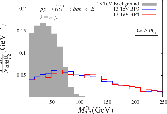
Figure 8: distributions of the harder lepton (left) and the distributions (right) and dileptonic stransverse mass for the background and the signals (in benchmark scenarios BP-3 and BP-4) in the 2 -jet +2 lepton+ final state arising from decays of for the case . - •
(figure 3)
In this case the overwhelmingly dominant decay mode is . As mentioned earlier, the emitted electron (positron) could have a very high as is evident from the left panel of figure 9. A strong cut (200 GeV) on the electron can thus be easily afforded to suppress the SM background effectively. Similar to the case of figure 7, the distributions of MET (of spurious origin) for the present case are presented in the right panel of figure 9. Again, the MET distributions peak at small values ( GeV), as expected and explained earlier. Again, possible reconstructions of -s in the invariant mass distributions of suitable pairs of -jet-electron (positron) systems are on the cards. We would touch briefly on this issue later in this section.
It is also important to note that ATLAS has performed a search for RPV stops in this channel [141]. Our analysis strategy is somewhat different from what they have chosen. ATLAS uses a cut on hadronic transverse momentum TeV and requires the invariant masses of the -lepton pairs to be within of each other. We find that the simple cut on electron momentum suppresses the background equally well and should be robust even at high pileup conditions.


Before going into the assessment of the signal significance, we mention below some issues of interest/importance pertaining to possible final states in these two cases.
- •
For both (section VI.1) and (section VI.2), we have only looked into the 2 -jet+2 lepton+ final state arising from pair production. However, the first scenario is phenomenologically richer as it can yield multi-lepton signals with 4-6 leptons in the final states when -s and -s decay via cascades involving the heavier neutralinos and charginos that in turn decay to SM bosons (see tables 3 and 5). Some corroborative analyses can take advantage of such inclusive final states comprising of 4 to 6 leptons along with -jets and MET.
- •
Furthermore, such a possibility could help differentiate from the two distinct scenarios considered in this work. For , in addition to the 2 -jets + final state out of which a pair of could be reconstructed, there would also be multi-lepton final states where leptons other than would appear. This is sharp contrast to the regime with .
- •
A final state like 2 -jets + arising from the decays of -s would be ideally free from any MET. However, as pointed out earlier, in reality, mis-measurements of various momenta may give rise to low to moderate amount of MET thus rendering the final state arising from a pair of -s to be similar to that is obtained from pair-production in a part of the phase space. This gives rise to some legitimate concern as to how efficiently the signature of -s could be deciphered, given the rates for such a final state originating in pair production would be, in general, large thanks to smaller mass of .
Such contaminations, however, can be avoided to a reasonable extent by imposing hard cuts on the minimum of the leading electrons as guided by the lepton distributions in the left panels of figures 6 and 7 (for ) and figures 8 and 9 (for ). In addition, imposition of a cut on the maximum allowed MET could effectively restrict the contamination thus allowing for a more efficient reconstruction of . By studying the MET distributions presented in the right panels of figures 7 and 9, we find an optimal value of this cut to be 50 GeV that helps retain a healthy number of ‘signal’ events with low , a characteristic of such a final state originating in the decays of .


Figure 10: Invariant mass distributions for the appropriate pairs of -jet-eletron (positron) systems (with low MET characteristic of -parity violating decays of to a bottom quark and an electron (positron)) for (left) and (right). The distributions are obtained by imposing 200 GeV for the leading electron and 50 GeV. In figure 10 we present the invariant mass distributions of appropriately chosen pairs of -jet and an electron (positron). Guided by figures 7 and 9, a high threshold of 200 GeV for the leading electron is demanded along with requiring a 50 GeV to ensure that we mostly confine ourselves to the signal region. The left (right) panel of figure 10 represent the case with (). We find that in both cases clear peaks at show up thus raising the hope that not only -s could be discovered in this mode but also a reliable estimate of its mass would be possible.
Before we close this subsection we like to mention that although we have only discussed two broad scenarios, i.e., and , other intermediate situations are all a priori viable. However, the expectations under those scenarios could be substantiated in a straightforward manner from the two cases we present. For example, an increase in value of from that in Case 1 would result in suppression of the branching fractions to Higgsino-like neutralinos and charginos. With increasing , at some point, these decay-modes (see table 3) would be closed for and BR() = 1. At the same time, branching fractions to the Higgsino-like states for would also get suppressed before these decay-modes get completely closed as it happens in Case 2. A detail study of possible correlations among the event rates in various final states could, in principle, shed light on the relative value of with respect to and . However, this is beyond the scope of the present work.
VII.5 Signal significance and the reach
The signal significance () is estimated using the expression [142]
| (60) |
which is appropriate for the situation with small number of events (in particular when the number of background events is less than 50). Equation (60) is based on likelihood-ratios and follows from the Poisson distribution. Here, and stand for the numbers of the signal and the background events, respectively after imposition of the set of optimal cuts discussed in section VII.4. The -factors for are computed using Prospino2 (v2.1) [132, 133].
We now estimate the required integrated luminosities for a reach of and in the four benchmark scenarios we consider. The final states we focus on are 2 -jets+2 leptons+ and , which stem from the decay of and , respectively.
| - | BP1 | BP2 | BP3 | BP4 |
|---|---|---|---|---|
| (fb) | 428.9 | 463.4 | 193.0 | 73.6 |
| Cut acceptance for signal | 1.6 | 4.4 | ||
| ( 200 GeV for BP1 and BP2) | ||||
| ( GeV for BP3 and BP4) | ||||
| Required for significance | 256.0 | 316 | 2350.0 | 3000 (3) |
For the first case (see table 10) the dominant background comes from pair production which subsequently decays to the 2 -jet+2 lepton+ final state. An appropriate -factor of 1.6 is used to derive the NLO cross sections from the LO ones for -pair production.
We note that a signal significance can be achieved for BP-1 and BP-2, with an integrated luminosity around 100 fb-1. To achieve a similar significance for BP-3 and BP-4, one has to wait for a much higher accumulated luminosity, for example, 500 fb-1 and 3000 fb-1, respectively at TeV.
| - | BP1 | BP2 | BP3 | BP4 |
|---|---|---|---|---|
| (fb) | 7.83 | 8.69 | 8.45 | 8.48 |
| Cut acceptance for signal | 1.96 | 5.26 | 1.9 | 1.9 |
| ( GeV, 50 GeV) | ||||
| Required for significance | 501.23 | 63.92 | 6.85 | 6.61 |
In table 11 we present the required luminosities for a reach of for the four benchmark points. The dominant SM background comes from production followed by giving rise to pairs. This can be efficiently suppressed by using an on-shell -veto for the pairs, as discussed in section VII.3. Thus, as can be seen from this table, a significance can be obtained with an integrated luminosity as low as fb-1 for the benchmark scenarios BP-3 and BP-4 with TeV. In addition, we also study the distribution, i.e., the scalar sum of the of the pair and the reconstructed -jets and the improvements are marginal. The wildly varying integrated luminosities across the benchmark points are the artifact of varying branching fractions that are instrumental, as has been pointed out in section VI.


Figure 11 summarises the mass-reach for the two top squarks with varying accumulated integrated luminosities (or, in other words, luminosity required to probe a certain top squark mass) at the 13 TeV LHC. The left panel illustrates the case for in the final state 2+2 lepton+ in BP-2 while the right one does the same for via 2+ final state in BP-4. As indicated by tables 10 and 11, figure 11 also reveals that has a significantly better reach compared to with the final states under consideration. This may lead to a tantalising possibility of discovering of such a scenario much earlier than and the former could guide us to find the latter. We observe that at the 13 TeV LHC and with the mass-reaches for and are around 575 (750) GeV and 1.2 (1.4) TeV respectively, with an integrated luminosity of 300 (3000) fb-1.
VIII The ‘stealth’ top squark scenario
The SUSY model under consideration, with super-light carriers of MET like and an MeV neutralino LSP () can easily conceive a rather low mass top squark lying right in the so-called ‘stealth’ window of [78]. As discussed in section V.3, the experimental lower bound on is more stringent considering its decay modes. Hence we choose to be the lightest top squark (). A benchmark point can be obtained by choosing GeV2. This results in GeV. Such a light top squark cannot provide enough correction to the Higgs mass. Hence we choose a relatively large value of (=1.28) so that the radiatively generated additional quartic contributions could lift the Higgs boson mass to the observed range. All other parameters are fixed at the values mentioned in BP-1 (see table 2). Note that the additional tree level contribution proportional to the neutrino Yukawa coupling ‘’ remains small (even for its order one value) because of large values of that we require. As a result, mostly decays to and with 85% and 15% branching fractions, respectively. The possible final state topologies are exactly the same as those result from top quark pair production.
We again analyse the final state with 2 -jets+ 2 leptons+. We checked that the distributions of various kinematic observables look very similar for the signal and the background, which is something literally expected of a ‘stealth’ top squark and what makes it so elusive. In figure 12 we present the distribution of the harder lepton (left panel) and the distribution (right panel) which clearly demonstrate how similar the behaviors of the SM background and the signal could get. In this context, techniques to exploit differences in spin-correlations inherent to and systems [82], use of various transverse mass variables [143] including the one like in the dileptonic decay channel [144], incorporating a new variable like ‘topness’ [145] using asymmetric decays of the top squarks have been proposed to study the ‘stealth’ top squark regime in search for an improved sensitivity. Clearly the issue demands dedicated addressal which is beyond the scope of the present discussion.


IX Summary and conclusions
We study a lepton number model augmented with a right handed neutrino superfield. The -charges are identified with the lepton numbers in such a way that the sneutrinos acquire large -s. Such large -s for sneutrinos are not prohibited since, in such a scenario, the same are not constrained by the Majorana masses of the neutrinos. In this paper, we choose to work in a basis in which only the electron type sneutrino acquires a nonzero whereas the -s of the other two sneutrinos are rotated away. This simple extension with a right handed neutrino superfield is rather interesting in the sense that the Higgs boson mass gets a tree level contribution which can be substantial in the low regime and for order one neutrino Yukawa coupling ‘’. Also present are the large one loop contribution to the Higgs boson mass arising from new couplings in the theory. Thus, one can easily accommodate a scenario where both top squarks are light. In addition, a very light bino-like neutralino comes out naturally in this scenario along with an active neutrino endowed with an appropriately small Majorana mass. Therefore, rich and interesting collider signatures are expected in such a scenario. The signature of a top squark decaying to a top quark and a neutralino and/or a neutrino is similar to the top quark pair production in the SM. Under favorable circumstances, top squark could also decay to a bottom quark and a chargino leading to a similar final state containing 2 -jets and 2 leptons along with MET. In this mode, top squark mass of around 575 (750) GeV can be probed with 300 (3000) of integrated luminosity.
Furthermore, in an -parity violating scenario such as ours, the charginos mix with the electron. The decay width of the top squark to a bottom quark and an electron (positron) is enhanced because of the enhanced coupling as well as an unsuppressed phase space. Hence we study in detail the final state with 2 -jets accompanied by an pair arising from such a dominant decay. We show that even when the top squark is heavy ( TeV), this particular channel could deliver a large signal significance with 300 (3000) of integrated luminosity.
In the model discussed in this work, only decays to . This is an artifact of no - mixing in the top squark sector. Also, note that the scenario prohibits decaying to or . The final state arising from both top squarks decaying to mode could carry MET which can only be of spurious origin (mis-measurements of various visible momenta, defects in the detector, etc.) and hence is characteristically small. This feature can be used to establish such a model and differentiate it from other competing ones. Due to a relatively clean final state and hence, a possibility to reconstruct the heavier top squark mass reasonably efficiently, such a state could be within an easier reach of the current LHC run when compared to its lighter peer. Such a scenario thus, gives rise to an interesting possibility that can be found much earlier than at the LHC and could carry a reliable hint as to where exactly to look for the latter. The signal region for is attributed with a much larger MET as is usual in searches for new heavy states in scenarios with a stable charge- and color-neutral particle(s). This is in sharp contrast with the case of in such a scenario.
Although the analyses in this work are presented in terms of two broad scenarios, viz., and , it is pointed out that the signatures discussed are robust under intermediate situations except for some obvious quantitative issues getting in. Simultaneous searches in various channels described in this work are expected to shed light on the detailed aspect of the spectrum and the involved new couplings of such a scenario.
Finally, we have demonstrated how the ‘stealth’ top squark can appear in our model naturally. However, probing such a window, 197 GeV 205 GeV [78] needs dedicated analysis which is an active area of research on its own merit. Overall, characteristic signatures for these light top squark states at the LHC even have the potential to discriminate between competing scenarios that may give rise to such a light pair of top squarks. In addition, such issues and projections are not readily available for 13/14 TeV run. Therefore, it is important to study all these issues at the dawn of 13 TeV run of the LHC.
Acknowledgements.
SC would like to thank the Council of Scientific and Industrial Research, Government of India for the financial support received as a Senior Research Fellow. It is a pleasure to thank Florian Staub for many helpful discussions regarding SARAH. SC would also like to thank Subhadeep Mondal, Arghya Choudhury and Amit Chakraborty for many helpful discussions. AD would like to thank the Department of Theoretical Physics, IACS for hospitality during the course of this work. SR acknowledges the hospitality of the University of Helsinki and Helsinki Institute of Physics where this work was initiated. KH and HW acknowledge support from the Academy of Finland (project no 137960).References
- [1] G. Aad et al. [ATLAS Collaboration], Phys. Lett. B 716 (2012) 1 [arXiv:1207.7214 [hep-ex]].
- [2] S. Chatrchyan et al. [CMS Collaboration], Phys. Lett. B 716 (2012) 30 [arXiv:1207.7235 [hep-ex]].
- [3] S. Chatrchyan et al. [CMS Collaboration], Eur. Phys. J. C 73 (2013) 9, 2568 [arXiv:1303.2985 [hep-ex]].
- [4] G. Aad et al. [ATLAS Collaboration], JHEP 1310 (2013) 130 [Erratum-ibid. 1401 (2014) 109] [arXiv:1308.1841 [hep-ex]].
- [5] G. Aad et al. [ATLAS Collaboration], JHEP 1409 (2014) 176 [arXiv:1405.7875 [hep-ex]].
- [6] P. Fayet, Phys. Lett. B 64 (1976) 159.
- [7] J. Polchinski and L. Susskind, Phys. Rev. D 26, 3661 (1982).
- [8] L. J. Hall, Mod. Phys. Lett. A 5 (1990) 467.
- [9] L. J. Hall and L. Randall, Nucl. Phys. B 352 (1991) 289.
- [10] I. Jack and D. R. T. Jones, Phys. Lett. B 457 (1999) 101 [hep-ph/9903365].
- [11] P. J. Fox, A. E. Nelson and N. Weiner, JHEP 0208 (2002) 035 [hep-ph/0206096].
- [12] A. E. Nelson, N. Rius, V. Sanz and M. Unsal, JHEP 0208 (2002) 039 [hep-ph/0206102].
- [13] Z. Chacko, P. J. Fox and H. Murayama, Nucl. Phys. B 706 (2005) 53 [hep-ph/0406142].
- [14] I. Antoniadis, K. Benakli, A. Delgado, M. Quiros and M. Tuckmantel, Phys. Lett. B 634, 302 (2006) [arXiv:hep-ph/0507192];
- [15] I. Antoniadis, K. Benakli, A. Delgado, M. Quiros and M. Tuckmantel, Nucl. Phys. B 744, 156 (2006) [arXiv:hep-th/0601003].
- [16] I. Antoniadis, K. Benakli, A. Delgado and M. Quiros, Adv. Stud. Theor. Phys. 2, 645 (2008) [arXiv:hep-ph/0610265].
- [17] G. D. Kribs, E. Poppitz and N. Weiner, Phys. Rev. D 78 (2008) 055010 [arXiv:0712.2039 [hep-ph]].
- [18] S. Y. Choi, M. Drees, A. Freitas and P. M. Zerwas, Phys. Rev. D 78 (2008) 095007 [arXiv:0808.2410 [hep-ph]].
- [19] S. D. L. Amigo, A. E. Blechman, P. J. Fox and E. Poppitz, JHEP 0901, 018 (2009) [arXiv:0809.1112 [hep-ph]];
- [20] K. Benakli and M. D. Goodsell, Nucl. Phys. B 816 (2009) 185 [arXiv:0811.4409 [hep-ph]].
- [21] A. E. Blechman, Mod. Phys. Lett. A 24 (2009) 633 [arXiv:0903.2822 [hep-ph]].
- [22] G. Belanger, K. Benakli, M. Goodsell, C. Moura and A. Pukhov, JCAP 0908 (2009) 027 [arXiv:0905.1043 [hep-ph]].
- [23] K. Benakli and M. D. Goodsell, Nucl. Phys. B 830 (2010) 315 [arXiv:0909.0017 [hep-ph]].
- [24] A. Kumar, D. Tucker-Smith and N. Weiner, Lepton Flavor Violation in the MRSSM,” JHEP 1009 (2010) 111 [arXiv:0910.2475 [hep-ph]].
- [25] B. A. Dobrescu and P. J. Fox, Eur. Phys. J. C 70 (2010) 263 [arXiv:1001.3147 [hep-ph]].
- [26] K. Benakli and M. D. Goodsell, Nucl. Phys. B 840 (2010) 1 [arXiv:1003.4957 [hep-ph]].
- [27] S. Y. Choi, D. Choudhury, A. Freitas, J. Kalinowski, J. M. Kim and P. M. Zerwas, Supersymmetry at Colliders,” JHEP 1008 (2010) 025 [arXiv:1005.0818 [hep-ph]].
- [28] L. M. Carpenter, JHEP 1209 (2012) 102 [arXiv:1007.0017 [hep-th]].
- [29] G. D. Kribs, T. Okui and T. S. Roy, Phys. Rev. D 82 (2010) 115010 [arXiv:1008.1798 [hep-ph]].
- [30] S. Abel and M. Goodsell, JHEP 1106 (2011) 064 [arXiv:1102.0014 [hep-th]].
- [31] K. Benakli, M. D. Goodsell and A. -K. Maier, Nucl. Phys. B 851 (2011) 445 [arXiv:1104.2695 [hep-ph]].
- [32] J. Kalinowski, Acta Phys. Polon. B 42 (2011) 2425.
- [33] K. Benakli, Fortsch. Phys. 59 (2011) 1079 [arXiv:1106.1649 [hep-ph]].
- [34] C. Frugiuele and T. Gregoire, Phys. Rev. D 85 (2012) 015016 [arXiv:1107.4634 [hep-ph]].
- [35] H. Itoyama and N. Maru, Gaugino Masses of Mixed Majorana-Dirac Type,” Int. J. Mod. Phys. A 27 (2012) 1250159 [arXiv:1109.2276 [hep-ph]].
- [36] C. Brust, A. Katz, S. Lawrence and R. Sundrum, JHEP 1203 (2012) 103 [arXiv:1110.6670 [hep-ph]].
- [37] K. Rehermann and C. M. Wells, arXiv:1111.0008 [hep-ph].
- [38] R. Davies and M. McCullough, Phys. Rev. D 86 (2012) 025014 [arXiv:1111.2361 [hep-ph]].
- [39] E. Bertuzzo and C. Frugiuele, JHEP 1205 (2012) 100 [arXiv:1203.5340 [hep-ph]].
- [40] R. Davies, JHEP 1210 (2012) 010 [arXiv:1205.1942 [hep-th]].
- [41] R. Argurio, M. Bertolini, L. Di Pietro, F. Porri and D. Redigolo, JHEP 1208 (2012) 086 [arXiv:1205.4709 [hep-th]].
- [42] M. D. Goodsell, JHEP 1301 (2013) 066 [arXiv:1206.6697 [hep-ph]].
- [43] R. Fok, G. D. Kribs, A. Martin and Y. Tsai, Phys. Rev. D 87 (2013) 5, 055018 [arXiv:1208.2784 [hep-ph]].
- [44] R. Argurio, M. Bertolini, L. Di Pietro, F. Porri and D. Redigolo, JHEP 1210 (2012) 179 [arXiv:1208.3615 [hep-th]].
- [45] C. Frugiuele, T. Gregoire, P. Kumar and E. Ponton, JHEP 1303 (2013) 156 [arXiv:1210.0541 [hep-ph]].
- [46] C. Frugiuele, T. Gregoire, P. Kumar and E. Ponton, JHEP 1305 (2013) 012 [arXiv:1210.5257 [hep-ph]].
- [47] K. Benakli, M. D. Goodsell and F. Staub, JHEP 1306 (2013) 073 [arXiv:1211.0552 [hep-ph]].
- [48] F. Riva, C. Biggio and A. Pomarol, JHEP 1302 (2013) 081 [arXiv:1211.4526 [hep-ph]].
- [49] H. Itoyama and N. Maru, Phys. Rev. D 88 (2013) 025012 [arXiv:1301.7548 [hep-ph], arXiv:1301.7548 [hep-ph]].
- [50] H. Itoyama and N. Maru, arXiv:1312.4157 [hep-ph].
- [51] P. Agrawal and C. Frugiuele, JHEP 1401 (2014) 115 [arXiv:1304.3068 [hep-ph], arXiv:1304.3068].
- [52] S. Chakraborty and S. Roy, matter in an lepton number model,” JHEP 1401 (2014) 101 [arXiv:1309.6538 [hep-ph]].
- [53] C. Csaki, J. Goodman, R. Pavesi and Y. Shirman, Phys. Rev. D 89 (2014) 5, 055005 [arXiv:1310.4504 [hep-ph]].
- [54] E. Dudas, M. Goodsell, L. Heurtier and P. Tziveloglou, Nucl. Phys. B 884 (2014) 632 [arXiv:1312.2011 [hep-ph]].
- [55] H. Beauchesne and T. Gregoire, JHEP 1405 (2014) 051 [arXiv:1402.5403 [hep-ph]].
- [56] E. Bertuzzo, C. Frugiuele, T. Gregoire and E. Ponton, JHEP 1504 (2015) 089 [arXiv:1402.5432 [hep-ph]].
- [57] K. Benakli, M. Goodsell, F. Staub and W. Porod, Phys. Rev. D 90, 045017 (2014) [arXiv:1403.5122 [hep-ph]].
- [58] S. Chakraborty, D. K. Ghosh and S. Roy, JHEP 1410 (2014) 146 [arXiv:1405.6967 [hep-ph]].
- [59] M. D. Goodsell and P. Tziveloglou, Nucl. Phys. B 889 (2014) 650 [arXiv:1407.5076 [hep-ph]].
- [60] S. Ipek, D. McKeen and A. E. Nelson, Phys. Rev. D 90 (2014) 7, 076005 [arXiv:1407.8193 [hep-ph]].
- [61] D. Busbridge, arXiv:1408.4605 [hep-ph].
- [62] P. Dießner, J. Kalinowski, W. Kotlarski and D. Stöckinger, JHEP 1412 (2014) 124 [arXiv:1410.4791 [hep-ph]].
- [63] S. Chakraborty, A. Datta and S. Roy, JHEP 1502 (2015) 124 [arXiv:1411.1525 [hep-ph]], Erratum to be published.
- [64] A. E. Nelson and T. S. Roy, Phys. Rev. Lett. 114 (2015) 201802 [arXiv:1501.03251 [hep-ph]].
- [65] S. P. Martin, arXiv:1506.02105 [hep-ph].
- [66] J. Berger, J. A. Dror and W. H. Ng, arXiv:1506.08213 [hep-ph].
- [67] M. D. Goodsell, M. E. Krauss, T. Müller, W. Porod and F. Staub, arXiv:1507.01010 [hep-ph].
- [68] T. Schwetz, M. Tortola and J. W. F. Valle, New J. Phys. 13 (2011) 063004 [arXiv:1103.0734 [hep-ph]].
- [69] T. Schwetz, M. Tortola and J. W. F. Valle, New J. Phys. 13 (2011) 109401 [arXiv:1108.1376 [hep-ph]].
- [70] D. V. Forero, M. Tortola and J. W. F. Valle, Phys. Rev. D 86 (2012) 073012 [arXiv:1205.4018 [hep-ph]].
- [71] M. C. Gonzalez-Garcia, M. Maltoni, J. Salvado and T. Schwetz, JHEP 1212 (2012) 123 [arXiv:1209.3023 [hep-ph]].
- [72] W. Porod, M. Hirsch, J. Romao and J. W. F. Valle, Phys. Rev. D 63 (2001) 115004 [hep-ph/0011248].
- [73] F. Staub, arXiv:0806.0538 [hep-ph].
- [74] F. Staub, Comput. Phys. Commun. 184, pp. 1792 (2013) [Comput. Phys. Commun. 184, 1792 (2013)] [arXiv:1207.0906 [hep-ph]].
- [75] F. Staub, arXiv:1503.04200 [hep-ph].
- [76] D. Curtin, P. Meade and P. J. Tien, Phys. Rev. D 90 (2014) 11, 115012 [arXiv:1406.0848 [hep-ph]].
- [77] J. Beuria, A. Chatterjee, A. Datta and S. K. Rai, arXiv:1505.00604 [hep-ph].
- [78] G. Aad et al. [ATLAS Collaboration], arXiv:1506.08616 [hep-ex].
- [79] J. Fan, M. Reece and J. T. Ruderman, JHEP 1111 (2011) 012 [arXiv:1105.5135 [hep-ph]].
- [80] C. Csaki, L. Randall and J. Terning, Phys. Rev. D 86 (2012) 075009 [arXiv:1201.1293 [hep-ph]].
- [81] J. Fan, M. Reece and J. T. Ruderman, JHEP 1207 (2012) 196 [arXiv:1201.4875 [hep-ph]].
- [82] Z. Han and A. Katz, arXiv:1310.0356 [hep-ph].
- [83] M. Czakon, A. Mitov, M. Papucci, J. T. Ruderman and A. Weiler, Phys. Rev. Lett. 113 (2014) 20, 201803 [arXiv:1407.1043 [hep-ph]].
- [84] T. Eifert and B. Nachman, Phys. Lett. B 743 (2015) 218 [arXiv:1410.7025 [hep-ph]].
- [85] S. Chakraborty, AseshKrishna Datta, Katri Huitu, Sourov Roy, Harri Waltari, Work in progress.
- [86] H. K. Dreiner, M. Hanussek, J. S. Kim and S. Sarkar, Phys. Rev. D 85 (2012) 065027 [arXiv:1111.5715 [hep-ph]].
- [87]
[ATLAS Collaboration],
ATLAS-CONF-2013-037, ATLAS-COM-CONF-2013-038.
- [88]
[CMS Collaboration],
CMS-PAS-SUS-12-023.
- [89]
The ATLAS collaboration,
ATLAS-CONF-2013-061, ATLAS-COM-CONF-2013-071.
- [90] S. Chatrchyan et al. [CMS Collaboration], Eur. Phys. J. C 73 (2013) 12, 2677 [arXiv:1308.1586 [hep-ex]].
- [91] The ATLAS collaboration, ATLAS-CONF-2015-015, ATLAS-COM-CONF-2015-017.
- [92] V. Khachatryan et al. [CMS Collaboration], Phys. Lett. B 739 (2014) 229 [arXiv:1408.0806 [hep-ex]].
- [93] R. Barbier, C. Berat, M. Besancon, M. Chemtob, A. Deandrea, E. Dudas, P. Fayet and S. Lavignac et al., Phys. Rept. 420 (2005) 1 [hep-ph/0406039].
- [94] S. Ambrosanio, G. L. Kane, G. D. Kribs, S. P. Martin and S. Mrenna, Phys. Rev. D 54 (1996) 5395 [hep-ph/9605398].
- [95] J. F. Gunion and H. E. Haber, Nucl. Phys. B 272 (1986) 1 [Erratum-ibid. B 402 (1993) 567].
- [96] I. Low, Phys. Rev. D 88 (2013) 9, 095018 [arXiv:1304.0491 [hep-ph]].
- [97] G. Aad et al. [ATLAS Collaboration], Phys. Rev. Lett. 114 (2015) 14, 142001 [arXiv:1412.4742 [hep-ex]].
- [98] G. Aad et al. [ATLAS Collaboration], JHEP 1406 (2014) 124 [arXiv:1403.4853 [hep-ex]].
- [99] V. Khachatryan et al. [CMS Collaboration], Phys. Lett. B 739 (2014) 229 [arXiv:1408.0806 [hep-ex]].
- [100] H. K. Dreiner, K. Nickel, F. Staub and A. Vicente, Phys. Rev. D 86 (2012) 015003 [arXiv:1204.5925 [hep-ph]].
- [101] A. Datta and B. Mukhopadhyaya, Phys. Rev. Lett. 85 (2000) 248 [hep-ph/0003174].
- [102] S. P. Das, A. Datta and S. Poddar, Phys. Rev. D 73 (2006) 075014 [hep-ph/0509171].
- [103] A. Datta and S. Poddar, Phys. Rev. D 75 (2007) 075013 [hep-ph/0611074].
- [104] A. Datta and S. Poddar, Phys. Rev. D 79 (2009) 075021 [arXiv:0901.1619 [hep-ph]].
- [105] Z. Marshall, B. A. Ovrut, A. Purves and S. Spinner, Phys. Lett. B 732 (2014) 325 [arXiv:1401.7989 [hep-ph]].
- [106] R. Bose, A. Datta, A. Kundu and S. Poddar, Phys. Rev. D 90 (2014) 3, 035007 [arXiv:1405.1282 [hep-ph]].
- [107] E. J. Chun, S. Jung, H. M. Lee and S. C. Park, Phys. Rev. D 90 (2014) 11, 115023 [arXiv:1408.4508 [hep-ph]].
- [108] A. Choudhury and A. Datta, Mod. Phys. Lett. A 27 (2012) 1250188 [arXiv:1207.1846 [hep-ph]].
- [109] R. Grober, M. Muhlleitner, E. Popenda and A. Wlotzka, arXiv:1408.4662 [hep-ph].
- [110] G. Ferretti, R. Franceschini, C. Petersson and R. Torre, Phys. Rev. Lett. 114 (2015) 201801 [arXiv:1502.01721 [hep-ph]].
- [111] G. Belanger, D. Ghosh, R. Godbole and S. Kulkarni, arXiv:1506.00665 [hep-ph].
- [112] S. Chatrchyan et al. [CMS Collaboration], Phys. Rev. Lett. 111 (2013) 22, 221801 [arXiv:1306.6643 [hep-ex]].
- [113] G. Aad et al. [ATLAS Collaboration], Phys. Rev. D 90 (2014) 5, 052008 [arXiv:1407.0608 [hep-ex]].
- [114] A. Chakraborty, D. K. Ghosh, D. Ghosh and D. Sengupta, JHEP 1310 (2013) 122 [arXiv:1303.5776 [hep-ph]].
- [115] J. Eckel, S. Su and H. Zhang, arXiv:1411.1061 [hep-ph].
- [116] A. Chakraborty, D. K. Ghosh, S. Mondal, S. Poddar and D. Sengupta, Phys. Rev. D 91 (2015) 115018 [arXiv:1503.07592 [hep-ph]].
- [117] J. S. Kim, K. Rolbiecki, K. Sakurai and J. Tattersall, JHEP 1412 (2014) 010 [arXiv:1406.0858 [hep-ph]].
- [118] H. Abe, J. Kawamura and Y. Omura, arXiv:1505.03729 [hep-ph].
- [119] T. Han, S. Su, Y. Wu, B. Zhang and H. Zhang, arXiv:1507.04006 [hep-ph].
- [120] CMS Collaboration [CMS Collaboration], CMS-PAS-SUS-13-018.
- [121] W. Porod, Comput. Phys. Commun. 153 (2003) 275 [hep-ph/0301101].
- [122] W. Porod and F. Staub, Comput. Phys. Commun. 183 (2012) 2458 [arXiv:1104.1573 [hep-ph]].
- [123] W. Porod, F. Staub and A. Vicente, Eur. Phys. J. C 74 (2014) 8, 2992 [arXiv:1405.1434 [hep-ph]].
- [124]
P. Bechtle, O. Brein, S. Heinemeyer, G. Weiglein and K. E. Williams,
Comput. Phys. Commun. 181 (2010) 138
[arXiv:0811.4169 [hep-ph]].
- [125]
P. Bechtle, O. Brein, S. Heinemeyer, G. Weiglein and K. E. Williams,
Comput. Phys. Commun. 182 (2011) 2605
[arXiv:1102.1898 [hep-ph]].
- [126]
P. Bechtle, O. Brein, S. Heinemeyer, O. Stal, T. Stefaniak, G. Weiglein and
K. Williams,
PoS CHARGED 2012 (2012) 024
[arXiv:1301.2345 [hep-ph]].
- [127] P. Bechtle, O. Brein, S. Heinemeyer, O. Stal, T. Stefaniak, G. Weiglein and K. E. Williams, Eur. Phys. J. C 74 (2014) 3, 2693 [arXiv:1311.0055 [hep-ph]].
- [128] P. Bechtle, S. Heinemeyer, O. Stål, T. Stefaniak and G. Weiglein, Eur. Phys. J. C 74 (2014) 2, 2711 [arXiv:1305.1933 [hep-ph]].
- [129] P. Bechtle, S. Heinemeyer, O. Stål, T. Stefaniak and G. Weiglein, JHEP 1411 (2014) 039 [arXiv:1403.1582 [hep-ph]].
- [130] J. Alwall, R. Frederix, S. Frixione, V. Hirschi, F. Maltoni, O. Mattelaer, H.-S. Shao and T. Stelzer et al., JHEP 1407 (2014) 079 [arXiv:1405.0301 [hep-ph]].
- [131] J. Pumplin, D. R. Stump, J. Huston, H. L. Lai, P. M. Nadolsky and W. K. Tung, JHEP 0207 (2002) 012 [hep-ph/0201195].
- [132] W. Beenakker, M. Kramer, T. Plehn, M. Spira and P. M. Zerwas, Nucl. Phys. B 515 (1998) 3 [hep-ph/9710451].
- [133] W. Beenakker, R. Hopker and M. Spira, hep-ph/9611232.
- [134] T. Sjostrand, S. Mrenna and P. Z. Skands, JHEP 0605 (2006) 026 [hep-ph/0603175].
- [135] https://twiki.cern.ch/twiki/bin/view/LHCPhysics/TtbarNNLO#Top_quark_pair_cross_sections_at
- [136] J. M. Campbell and R. K. Ellis, Phys. Rev. D 62 (2000) 114012 [hep-ph/0006304].
- [137] S. Dawson, C. Jackson, L. H. Orr, L. Reina and D. Wackeroth, Phys. Rev. D 68 (2003) 034022 [hep-ph/0305087].
- [138] F. Febres Cordero, L. Reina and D. Wackeroth, Phys. Rev. D 78 (2008) 074014 [arXiv:0806.0808 [hep-ph]].
- [139] R. Frederix, S. Frixione, V. Hirschi, F. Maltoni, R. Pittau and P. Torrielli, JHEP 1109 (2011) 061 [arXiv:1106.6019 [hep-ph]].
- [140] http://www.hep.phy.cam.ac.uk/~lester/mt2/
- [141] The ATLAS collaboration [ATLAS Collaboration], ATLAS-CONF-2015-015.
- [142] D. G. d’Enterria et al. [CMS Collaboration], J. Phys. G 34 (2007) 2307.
- [143] W. S. Cho, J. S. Gainer, D. Kim, K. T. Matchev, F. Moortgat, L. Pape and M. Park, JHEP 1505 (2015) 040 [arXiv:1411.0664 [hep-ph]].
- [144] C. Kilic and B. Tweedie, JHEP 1304 (2013) 110 [arXiv:1211.6106 [hep-ph]].
- [145] M. L. Graesser and J. Shelton, Phys. Rev. Lett. 111 (2013) 12, 121802 [arXiv:1212.4495 [hep-ph]].