Hindered M1 Radiative Decay of from Lattice NRQCD
Abstract
We present a calculation of the hindered M decay rate using lattice non-relativistic QCD. The calculation includes spin-dependent relativistic corrections to the NRQCD action through in the quark’s relative velocity, relativistic corrections to the leading order current which mediates the transition through the quark’s magnetic moment, radiative corrections to the leading spin-magnetic coupling and for the first time a full error budget. We also use gluon field ensembles at multiple lattice spacing values, all of which include , , and quark vacuum polarisation. Our result for the branching fraction is , which agrees with the current experimental value.
pacs
12.38.Gc, 13.20.Gd, 13.40.Hq, 14.40.PqI Introduction
Quantum Chromodynamics (QCD) has been accepted as the theory describing the strong force of nature ever since the discovery of the . Since then, there has been a long history of using the spectrum and decays of heavy quarkonia in order to understand QCD, heavy quarkonia being the ideal theoretical testing grounds when using potential models, and more recently, lattice QCD. Heavy quarkonium states below threshold are very narrow, and electromagnetic transition rates are therefore significant. Comparing the theoretical and experimental rates for these decays then provides a very clear test of our understanding of the internal structure of heavy quarkonia.
A certain class of electromagnetic transitions between quarkonium states, known as hindered M transitions, require a spin-flip between different radial excitations and are particularly sensitive to small relativistic effects [1] which can illuminate the dynamics of the initial and final state systems. These hindered M transitions still remain a challenge from both the experimental and theoretical perspective. Within the bottomonium sector, such decays include the radiative transition, where BaBar measured [2] in .
On the theory side, hindered M decays have been nortoriously difficult to pin down from within a potential model framework [1], where systematic errors are hard to quantify and branching fractions ranging from to are found. The reasons for the difficulty in accurately predicting these decays from within a potential model will be discussed in Section VI. The continuum effective field theory approach called potential NRQCD (pNRQCD) has been used to predict radiative bottomonium decays, including M transitions. While these calculations have become quite precise for the allowed S S M transitions, the results for hindered M transitions are dominated by theoretical uncertainties and presently can only give an order-of-magnitude estimate [3, 4].
Lattice NRQCD is a first principles tool that has been systematically improved by the HPQCD collaboration and can aid in reliably pinning down this difficult to predict decay. Using this formalism, one can accurately overcome each of the issues arising from within a potential model framework. Previous exploratory work on this decay in a lattice NRQCD framework was done in [5, 6]. We make a number of improvements to those studies so that an accurate calculation can be done, complete with a full error budget. Some of these improvements include using one-loop radiative corrections in the NRQCD action and we show in Section V that these decays are very sensitive to a subset of these radiative corrections.
This paper is organised as follows. In Section II we set up notation and formulae relevant to this decay, and in Section III we give details of the computational setup including a discussion of states in NRQCD at non-zero momentum. In Section IV the different currents mediating this transition in NRQCD are shown and the perturbative calculation of the matching coefficient from the leading order current to full QCD is performed. Finally, analysis of the decay rate with a full error budget is given in Section V. We conclude with a discussion in Section VI.
II Decay Rates for Radiative Transitions
BaBar has measured the branching fraction of the decay as [2], which when combined with the total width keV [7], gives the decay rate keV. The large errors on the branching fraction are due to the difficulty in isolating the small signal from other nearby photon lines (, ) and from the large background in the energy spectrum of inclusive decays [8].
We want to perform an accurate and reliable theoretical calculation to compare to this experimental result. Computation of the theoretical decay rate requires the matrix element of the appropriate operator between the and states as input. In a Lorentz invariant theory, using the fact that the matrix element transforms as a vector under parity (and parity invariance of our theory), the only possible decomposition of the matrix element is
| (1) |
where is the photon momentum, is the polarisation vector of the and by momentum conservation. Using time reversal invariance, one can show that is real [9]. As the is a bound state, this M (spin-flip) transition can occur by flipping the spin on either the quark or the antiquark. Since this is a symmetric process, the form factor resulting from coupling the current to the quark or to the anti-quark is then identical. In our lattice calculation we only couple the current to the quark (c.f. Sec. IV) and actually compute .
The decay rate can now be written as
| (2) |
where is the fine structure constant, is the quark charge in units of (i.e., for -quarks) and by energy conservation, ensuring that the photon is on-shell with . Thus, from the theoretical perspective, the most challenging part of calculating the decay rate from first principles is computing the single unknown dimensionless hadronic form factor , which encodes the nonperturbative effects of QCD. This quantity can be calculated in lattice QCD, and this study will focus on the computation of .
Using the experimental value of the decay rate mentioned above, as well as MeV measured from experiment [2] and , we infer
| (3) |
This form factor can be directly compared to . From now on, we will drop the subscript to avoid superfluous notation.
III Computational Details
III.1 Second Generation Gluon Ensembles
Our calculation uses gauge field configurations generated by the MILC collaboration [10]. For the gauge fields, they used the tadpole-improved Lüscher-Weisz gauge action, fully improved to . This is possible as the gluon action has coefficients corrected perturbatively through , including pieces proportional to the number of quark flavours in the sea [11]. These ensembles are said to have flavours in the sea, the up and down quarks (treated as two degenerate light quarks with mass ), the strange quark, and the charm quark. The sea quarks are included using the HISQ formulation of fermions [12], fully improved to , removing one-loop taste-changing processes and possessing smaller discretisation errors compared to the previous staggered actions.
Five ensembles were chosen, spanning three lattice spacing and three values of , so that any dependence on the lattice spacing and sea quark mass could be fit and extrapolated to the physical limit. Details are given in Table 1. Due to the computational expense, most of the ensembles use heavier than in the real world; however one of the ensembles used in this study (set in Table 1) has physical , enabling our calculations to be performed at the physical point and reducing uncertainties associated with unphysically heavy sea quark masses.
Successive configurations generated within each ensemble are expected to be correlated. These autocorrelations in meson correlators were studied in [13] for the ensembles in Table 1. There we find that the autocorrelations for bottomonium correlators are not appreciable and that the configurations can be treated as statistically independent. The ensembles have been fixed to Coulomb gauge to allow non-gauge invariant smearings to be used, helping extract precise results for the excited states in our calculation (c.f. Sec. III.4).
| Set | (fm) | ||||||
|---|---|---|---|---|---|---|---|
III.2 -quarks Using NRQCD
This study focuses purely on bottomonium processes, and information on these processes can be computed on the lattice using combinations of -quark propagators, calculated on the gluon ensembles listed in Table 1. As the -quark has a Compton wavelength of about fm, these lattices cannot resolve relativistic -quark formulations, owing to fm. However, it is well known that -quarks are very nonrelativistic inside their bound states (), and thus, using a nonrelativistic effective field theory (NRQCD) for bottomonium states is very appropriate. Within NRQCD, with expansion parameter (the velocity of the quark inside the bound state), one writes down a tower of operators to a certain order in allowing for a systematic inclusion of ever-decreasing relativistic corrections. This effective field theory is then discretised as lattice NRQCD [14]. There are a number of systematic improvements which need to be made in order to produce highly accurate results. These will be addressed shortly.
We use a lattice NRQCD action correct through , with additional spin-dependent terms11 1 The quantities relevant to this study are insensitive to the spin-independent terms within our precision. and include discretisation corrections. This lattice formalism has already been used successfully to study bottomonium , and wave mass splittings [13, 15], precise hyperfine splittings [16, 17], meson decay constants [18], and leptonic widths [19] and , meson mass splittings [17]. The Hamiltonian evolution equations can be written as
| (4) |
with
| (5) | ||||
| (6) |
The parameter is used to prevent instabilities at large momentum due to the kinetic energy operator. A value of is chosen for all values. A smearing function is used to improve projection onto a particular state in the lattice data. Using an array of smearing functions to improve the overlap with the ground state and the first excited state will prove crucial to obtaining accurate results for the decay. To evaluate the propagator, we use random wall sources that are implemented stochastically with white noise, significantly improving the precision of the S-wave states [13].
Here, is the bare quark mass, is the symmetric lattice derivative, with the improved version, and , are the lattice discretisations of , respectively. , are the improved chromoelectric and chromomagnetic fields, details of which can be found in [13]. Each of these fields, as well as the covariant derivatives, must be tadpole-improved using the same improvement procedure as in the perturbative calculation of the matching coefficients [20, 13] (thus removing unphysical tadpole diagrams from using the Lie group element rather than the Lie algebra element in the construction of the lattice field theory). We take the mean trace of the gluon field in Landau gauge, , as the tadpole parameter, calculated in [13, 18].
The matching coefficients in the above Hamiltonian take into account the high-energy UV modes from QCD processes that are not present in NRQCD. Each can be expanded perturbatively as and, after tadpole improvement, we expect the radiative corrections to be . Each can then be fixed by matching a particular lattice NRQCD formalism22 2 Changing the NRQCD action can modify the Feynman rules used in the computation of in perturbation theory, in general changing its value. to full continuum QCD. These corrections have previously been computed [20, 13]. Alternatively, particular ’s can be tuned nonperturbatively, which we discuss in Section V.2.9.
A high-precision calculation with a reliable error budget will require knowledge of at least the corrections to the matching coefficients. For example, when tuning the quark mass fully nonperturbatively in NRQCD, one computes the kinetic mass of a hadron33 3 The static mass (the energy corresponding to zero-spatial momentum) in lattice NRQCD [13] is shifted due to the removal of the mass term from the Hamiltonian and so one can only tune static mass differences fully nonperturbatively. [13]. This kinetic mass depends on the internal kinematics of the hadron, and hence on the terms , , and in the Hamiltonian. Using the one-loop corrected coefficients to these terms has a small but visible effect on the kinetic masses and hence on the value of the tuned [13].
In addition to this, for an NRQCD action with , the kinetic mass for the is actually found to be larger than that of the [13], opposite to what is seen at zero momentum and, more importantly, in experiment. The explanation is that the term gives rise to the hyperfine splitting, and the splitting from this term is correctly included in the static mass (the mass at zero energy, offset due to removing the mass term from the Lagrangian). However, relativistic corrections to (the term proportional to in the Hamiltonian above) are needed to correctly feed this splitting into the kinetic mass. On a fine lattice, a value of and was needed to yield a hyperfine splitting using kinetic masses which agreed with experiment within errors [16]. In order to remove the sensitivity to the term when tuning , one does not use the kinetic mass of a single state, but the spin-averaged kinetic mass of the and [13, 21]. Including terms in the evolution equations makes the kinetic mass lower than that of the , as they include relativistic corrections to the term. The spin-averaged kinetic mass gets smaller and the bare quark mass gets larger [16].
The parameters used in this study are summarised in Table 2. There, and are the correct values for a NRQCD action [13], but the small changes to these coefficients in going to a NRQCD action have a negligible effect on the quantities studied here, as shown in Figure 7. While the values from ensembles and listed in Table 2 have all been tuned against the spin-averaged kinetic mass using the Hamiltonian above [16], the values from ensembles and were previously tuned without the terms [18]. Ensembles and are all coarse lattices and only differ by having different light quark masses in the sea. Ensemble has a correctly tuned for the Hamiltonian we use, corresponding to GeV. It is appropriate to tune the values on the other coarse lattices to match this physical value. Using the lattice spacings listed in Table 1, we find the values on ensemble and listed in Table 2. All these ensembles have essentially the same value of the lattice spacing, so the running of the bare mass is a negligible effect. This was observed with a Hamiltonian [13].
| Set | , | ||||||
|---|---|---|---|---|---|---|---|
Within NRQCD, the Dirac field can be written in terms of the quark and anti-quark as . The propagator is then found to be
where is the two-spinor component quark propagator and is the two-spinor component anti-quark propagator. hermicity becomes . As such, we write our interpolating operators as in Table 3 and then use the above decomposition, with suitable boundary conditions, to write the correlator in terms of .
III.3 Non-Integer Momentum on the Lattice
Using periodic boundary conditions (PBC) for the quark fields forces the momentum components to be , where is an integer. The issue with this is that processes which occur at a specific momentum, such as that needed for an on-shell photon in the form factor , cannot be reached at an integer-valued momentum. Here, we use “twisted boundary conditions” (BC) [22, 23] in order to find the matrix element at the physical point. There are some subtleties with using BC in our calculation that, to our knowledge, are not found in the literature, and we give an explicit example of the construction of our twisted correlators in Appendix B. As seen there, and confirmed by numerical data, the twisted and untwisted correlator data should agree (if the same momentum is used) on a configuration level if everything is done correctly.
In our calculations, we choose and only twist a single propagator so that . The choice of isotropic twist momentum that gives depends on the specific process under study and for the decay is found from (2) as:
| (7) |
yielding . We choose an isotropic momentum as it has been shown to reduce discretisation errors from rotational symmetry breaking [13]. Since static masses obtained from correlators at rest are shifted by an arbitrary value in NRQCD, tuning from lattice data would require a more lengthy computation of the kinetic masses. Instead, we use the experimental values of these masses [7] to tune and check that from the results.
III.4 Energies and Amplitudes from Lattice QCD
Extracting matrix elements on the lattice requires knowledge of the lattice amplitudes and energies corresponding to the states being studied. The lattice quantity which most naturally encodes information on these is the two-point correlator
| (8) |
Here, is the source time, are the smearing type (discussed below) and is the twisted momentum. After performing the Wick contractions with the bilinear operators listed in Table 3, the connected44 4 Disconnected diagrams for heavy quarkonia are expected to be negligible as they are suppressed by the heavy quark mass [9]. correlator has the form
where is the twisted propagator (c.f. Appendix B). We use smearing functions on the anti-quark field at the source and sink respectively. We employ hydrogen-like wavefunctions which have been successful in previous studies of -physics: , , . is the smearing radius, and we point the reader to [13] for further details on the smearings55 5 We use the smearing types as described in that reference.. The different smearing combinations used in this study give a matrix of correlators. We do not smear the quark fields due to complications on using twisted-smeared fields as outlined in Appendix B.
The two-point correlator in (8) can be spectrally decomposed as
| (9) |
where is the energy excitation of the interpolating operator used in the construction of the correlator and are the corresponding amplitudes, labelled by the smearing used at the source or sink. We are only interested in the first few excited states, so we do not need to worry about multiparticle states or the open -threshold. Our two-point correlators are propagated for a maximum of timeslices, as after this the locally smeared correlator on a fine lattice is largely saturated by the ground state. In addition, correlators were calculated with different time sources on each configuration in order to increase statistics. To avoid complications due to correlations between these time sources, correlators were then averaged over all sources on the same configuration.
We fit the matrix of correlators from using a simultaneous multi-exponential Bayesian fit [24, 25] to the spectral decomposition in (9). Different smearings give rise to different amplitudes and so we take priors on them to be . The priors on the ground state energies are estimated from previous results and given a suitably wide width [13]. For the zero momentum case, prior information tells us that the energy splittings are of the order MeV, while for the nonzero momentum case, priors of MeV are used (due to the inclusion of additional states in the correlator, see Sec. III.5). Logarithms of the energy splittings are taken in the fit to ensure that the ordering of states is preserved, helping the stability of the fit [25].
III.5 Energy Eigenstates in Lattice NRQCD
Theoretically, particle states living in the Hilbert space are classified in terms of invariant quantities within irreducible representations (irreps) of the symmetry group of a theory. For our calculation, two groups need to be considered: the Lorentz group and the continuous rotational group in three dimensions. Appendix A reviews the construction of the irreps of both these groups at zero and nonzero momentum.
As is well known, the irreps of the Lorentz group at rest are described by , where , are the total and third component of angular momentum respectively. is the parity quantum number and for quarkonia is the charge conjugation. The quantum numbers classify all particles seen in experiment to date [7].
However, the symmetry group of NRQCD is only the rotational group. At zero momentum, the states within such a theory are also described by . At nonzero momentum, the situation is significantly different, and the irreps are described by , where is an eigenvalue of the helicity operator . This has important consequences for the energy spectrum extracted from our lattice calculation (compare the zero and nonzero momentum lattice spectrum seen in Figures 1, 2) and therefore needs to be fully understood in order to have a reliable computation.
At rest the bilinear operators that we use in our calculation, listed in Table 3 with , overlap onto definite energy eigenstates respectively in the infinite volume continuum version of our theory (which is rotationally invariant) [26]. In Appendix A (as in [26]) it is shown that at nonzero momentum, is a helicity operator which creates a definite energy eigenstate, but creates an admixture of eigenstates, where these get contributions from values as listed in the third column of Table 3. The superscript on the represents the eigenvalue from the symmetry (a parity transformation followed by a rotation to bring the momentum direction back to the original direction) [26].
In the correlator data from using , guided by the experimental masses and this analysis, the lowest states in the spectrum should be , etc. whereas from using the lowest states in the spectrum should be , etc. These are the states which we see in our lattice spectrum at nonzero momentum.
The first three states extracted from the spectrum with the operator , are shown in Figures 1, 2 respectively. On the same plot, the solid lines represent the energy of the states according to a nonrelativistic, rotational dispersion relation reconstructed using the experimental masses, e.g., , where is the kinetic mass which we set equal to the experimental mass, and is the static mass offset due to neglecting the mass term in the NRQCD Hamiltonian. We find in the correlator data from the operator by taking the ground state lattice energy at zero momentum and finding the shift in the static mass as the difference . We then use this value of the shift to find , to be used in the above dispersion relation. We found the shift in the correlator data in the same way.
The important point to observe in these figures is that at nonzero momentum the energy of the first excited state is actually lower than the energy of the first excited state at zero-momentum, opposite to what one would expect from a dispersion relation. The reason is clear: at nonzero momentum energy eigenstates have definite helicity, not definite . Therefore our correlator data gets contributions from the states listed in Table 3.
We conclude that, as Figures 1 and 2 show, one has to be careful in equating the states found in NRQCD at nonzero momentum with continuum quantum numbers and also in extracting matrix elements involving a state inflight. However, here we only extract excited states at zero-momentum in order to avoid unnecesssary complications and to obtain high-precision results, which can be muddled when extracting excited states in flight due to the addition of extra states in the spectrum and their small overlap factors as described in Appendix A. After our analysis, we can then be sure that we have extracted the correct matrix element for the decay.
III.6 Matrix Elements from Lattice QCD
The simplest quantity which encodes information on a meson-to-meson decay matrix element from within lattice QCD is the three-point correlator
| (10) | ||||
where , are interpolating operators which create the initial state with polarisation and final state respectively, is the current which induces the transition with labelling the polarisation of the photon, and the twisted momenta are described in Sec. III.3. The three-point correlator is visualised as in Figure 3 where the three points in lattice units correspond to: the source point of the initial particle at time (equal to zero in (10)); the position and time of the current causing the transition at (, ); and the position and time of the final state at (, ). After performing Wick contractions on the three-point correlator the connected contribution, written in terms of NRQCD propagators as discussed in Section III.2, is
| (11) |
where the twisted propagator is defined in Appendix B. Direct computation of the propagator is unnecessarily expensive as we can use the sequential source technique (SST) [27, 9] to yield the desired propagator, which only requires one further evolution. There are two ways to package the propagator in the three-point correlator when using the SST. The first is called the fixed current method, which requires the insertion time to be fixed and for propagator in Figure 3 to be used as a source for propagator . However, this method does not scale well and is undesirably expensive for relativistic quark formalisms.
The second approach is called the fixed sink method. In this approach, one fixes the sink time and factorises (11) as
| (12) |
with
where we have written in terms of the twisted propagator that satisfies periodic boundary conditions and used the fact that commutes with the exponential as described in Appendix B. We have also used the NRQCD -hermicity conditions from Sec. III.2, and used because . We can obtain by using the twisted evolution equations with the source .
Clearly, the two methods should give the same correlator data as they only differ in how is packaged. We have checked this numerically and found it to be true on any given configuration up to machine precision. As the fixed sink method is more cost effective, this method was used for the calculation. Our program structure can be visualised in Figure 3. Propagator is generated with a smeared, random wall source at time and propagated to time where the sink smearing is applied. is found by using the source and evolving backwards in time using the twisted configurations to a time . Propagator is made from the same random wall as . We then combine propagator , and the current as in (12) to obtain the three-point correlator. We use the same time sources as in the two-point correlator and prior to fitting, all data is translated to a common .
The three-point correlator (10) can be related to matrix elements of the current by inserting a complete set of states [9]. By doing so, and using the rotational parameterisation of the overlaps as described in Appendix A, is seen to be anti-symmetric. We average over the six nonzero contributions using an isotropic momentum as
| (13) |

In addition, inserting the complete set of states also leads to the functional form of the fitting function
| (14) |
where and are amplitudes from the two-point fitting function in (9). The two-point and three-point correlators can be simultaneously fit to (9) and (14) respectively using multi-exponential chained [28], marginalised [29] Bayesian fitting. Chained, marginalised fitting has been shown to significantly decrease the fitting time and produce reliable, precise and accurate results if the data is in the limit of high statistics (Gaussianly distributed) [30]. We check that results are compatible from both with and without chained, marginalised fits on a subset of the data. We use a prior of for all and the same priors for the amplitudes and energies as in the two-point fits described in Sec. III.4. For each current, we obtain data for fixed and the same matrix of smearings as in the two-point correlators. This allows accurate extractions of the matrix element as it includes excited state contributions.
The use of a singular value decomposition stabilises the fit and is standard practice in the literature [28]. In our Bayesian fit, this is performed by setting a tolerance and replacing all eigenvalues of the correlation matrix smaller than this tolerance times the maximum eigenvalue to this value [28]. By doing so, this leads to larger errors in the fit results and so is a conservative step. We use a tolerance of .
The matrix element for the decay will be proportional to . By equating the fitting functions to their continuum correlator counterparts with conventional relativistic normalisation, parameterising our overlaps using rotational invariance with the initial particle at rest, we find
| (15) |
where is the twisted momentum described in Sec. III.3. Since the static masses obtained from an NRQCD calculation are shifted, as explained previously, we extract from using the same experimental masses as in Sec. II. A nonrelativistic dispersion relation was used to find , which is appropriate as shown in Figure 1.
IV M1 Radiative Decay Currents
In order to compute the form factor , we need to choose currents which will induce a hindered M radiative decay. Within a nonrelativistic framework, it is a standard result in the literature [31, 32, 33] that the leading order contribution to the matrix element is suppressed due to the orthogonality of the radial wavefunctions and relativistic corrections are necessary. This suppression introduces a sensitivity to a range of effects that we must test and quantify in order to perform an accurate calculation. The first of these effects is the fact that next-to-leading order current contributions are appreciable and we need to include them.
As we are using NRQCD to simulate the -quark, choosing the currents from a NRQCD and non-relativistic quantum electrodynamics (NRQED) effective field theory is most appropriate. This effective field theory can be found straightforwardly by extending the Lie algebra of NRQCD to a Lie algebra to produce NRQCD NRQED [3]. Then, in principle, one could discretise the theory and choose appropriate currents from the resulting operators. However, this introduces complications, e.g. the magnetic field only decouples from the chromomagnetic field to leading order in the lattice spacing, resulting in lattice artefact currents which are not present in the continuum. Calculating such currents would require more computational resources and make the computation of the matching coefficients more difficult.
Instead, we are free to choose the currents from the continuum NRQCD NRQED theory and renormalise these. It is important to understand the power counting in the NRQCD NRQED effective field theory in order to choose our currents appropriately. Given that NRQCD NRQED is a effective field theory, it has two expansion parameters. For NRQCD, we have the standard expansion parameter , where for bottomonium. The only scale available for the on-shell emitted photon is the photon’s energy GeV. Since the photon’s energy is the difference between the masses of two heavy S-wave quarkonia, it is of the order GeV. Thus we can expand our effective field theory in terms of only.
We summarise the power counting as
- •
.
- •
, .
- •
The standard QCD power counting rules for the QCD fields.
- •
The knowledge that when a derivative acts on the photon field, it gives a factor of and when acting on the quark field a factor of (as the valence quark knows nothing of the photon momentum in the initial quarkonium rest frame).
Ordering the operators that induce a M (spin-flip) transition from NRQCD NRQED, we find (to next-to-leading order for our decay and borrowing notation from [34])
| (16) |
Here, are all pure QCD covariant derivatives, fields marked QED (QCD) are the QED (QCD) fields and are the matching coefficients needed to reproduce full QCDQED from our effective theory. Using the power counting rules above, we find , , and . We can then factor out the photon and electric charge in order to derive the currents which give the decomposition of the matrix element in (1). For example, the operator gives rise to the current
We then write all currents as so that will be what enters the three-point correlator as in (12). We use the terminology that the form factor coming from the current is called , where the tilde implies we have factored off the matching coefficient from the form factor in the numerical calculation and this should be applied later in the analysis. Similar notation is used for the other currents and we refer to as unrenormalised form factors. The final form factor is .
It should be noted that there are other currents (suppressed by or ) that contribute to this decay and which might be of interest, notably, the QCD analogues of the , operators arising from choosing the electric (magnetic) fields in (16) to be gluon fields and the photon coming from the full covariant derivative. Other operators are those which only occur at loop level in the full QCD QED theory. These can be written as
| (17) |
When attempting power counting on the QCD operators above, it is helpful to draw the Feynman diagram that such an operator would produce. Essentially, we need to contract the gluon field with another, producing another factor of at least [14]. Consequently these operators are expected to be of order at most. We confirm numerically that the form factors from these QCD operators are suppressed as expected and they are negligible within the errors of our final results. Since occur only at loop level they are suppressed by relative to . We will introduce a systematic error for neglected currents in the final analysis.
IV.1 Matching Coefficients for the Currents
The matching coefficients, , appearing in the operators in (16) are needed to take into account the high-energy UV modes from processes in the full theory but not present in our effective field theory. They have the expansion . Here we compute the one loop correction to the coefficient from the leading order current. Following this, we estimate the errors from neglecting corrections that we do not calculate.
Our calculation of the one-loop coefficient is very similar to the computation of the one-loop correction of in [20]. Following that analysis, by matching the current from NRQCD + NRQED to continuum QCD+QED, we find
| (18) |
where is the coefficient of the first order correction to the quark’s magnetic moment, computed analytically in continuum QCD following standard techniques. As is UV finite, this allows us to directly equate results obtained on the lattice to those obtained in the continuum, since the difference between the schemes for UV regulation is then irrelevant. In the general matching procedure the continuum and lattice IR divergences cancel in the computation of the radiative correction; here, because of the standard Ward Identity, the continuum and lattice contributions to are separately finite.
, , are the renormalisation factors of the bare quark mass, the wavefunction and the current from (16). These are calculated in lattice NRQCD. We automatically generate the Feynman rules for a specific NRQCD action (along with the Symanzik-improved gluonic action) using the HiPPy package, then compute the numerical evaluation of these diagrams using the HPsrc package [35, 36]. We use the full NRQCD Hamiltonian with spin dependent pieces as defined in (6). Computation of and is identical to [20]. will get contributions from mean-field corrections which we denote as . We use the Landau mean link [37]. For the action that we use, the tadpole correction is [20]
| (19) |
The NRQCD diagrams contributing to are shown in Figure 4. Since we do not actually include the QED field in our calculation, there are no tadpole factors from this term. Note that Fig. 4(a) is generated by the current coming from being inserted at the vertex, and Figs. 4(b), 4(c) and 4(d) arise from mixing effects from the higher order currents (that we include in the calculation of the decay rate) from (16). Computation of the Feynman diagrams shown in Figs. 4(b), 4(c) and 4(d) is more involved than that of Fig. 4(a), so they are not included in this calculation, but we plan on computing them in future work. For now, we will introduce a systematic error from neglecting these contributions.


A breakdown of the numerical values of the various terms that enter for the masses that we use in this calculation is shown in Table 4. was computed for a range of masses (neglecting the mixing down) and we give these values in Table 5.
We show the values of with a smooth interpolating curve in Figure 5. This interpolating curve was chosen to be a polynomial in in order to reproduce the static limit as . To fit these values easily we increased the errors on the points returned by HPsrc to . We use a Bayesian fit to all points in Figure 5 against a polynomial in . We found the smallest and largest Gaussian Bayes Factor [24] when including all terms in the polynomial up to and including the quartic term. We used a prior for the constant piece as the polynomial of and priors for the coefficients of the pieces of .
IV.2 Systematic Error from Current Matching Coefficients
We need to include a systematic error from not knowing the matching coefficients in the currents to infinite precision. There are two distinct types of errors in this case: the first is from neglecting the corrections in and the corrections to the matching coefficients of the other currents; the second is from neglecting the mixing down effects on the values of used in the calculation. We will estimate each of these in turn.
To estimate the effect of neglecting the higher order corrections that we have not calculated, it is helpful to compare our result to the pure NRQED calculation of [34]. There, the authors find that the continuum QED contribution to their is the anomalous magnetic moment of the electron , while for us it is the anomalous magnetic moment of the quark . For the NRQED contribution, they find no IR log nor a constant piece and in their continuum approach the UV power law divergences may be omitted. Although we find no IR log in our data, we cannot neglect the UV power law divergence associated with the momentum cutoff. This shows up as a polynomial in as mentioned above. We observe that this lattice artefact contribution gives a negative contribution to the continuum value, as shown in Table 4, and for the range that we are interested in . As we are observing similar behaviour over this mass range as the pure NRQED calculation, we can use that calculation to estimate the error conservatively.
As shown in [34] and confirmed by the small values of our numerical data, the matching coefficients can actually be expanded in . In principle, the second order coefficient of could be , and then this contribution could be . As such, we allow for an additive systematic error (assumed to be correlated across all ensembles) of from not knowing higher order contributions to .
We have not included the contributions to the other matching coefficients in (16), namely , and . A difficult calculation would be necessary to determine them. Again, we use the equivalent parameters from the pure NRQED calculation [34] to estimate the systematic error. The pure NRQED equivalent of has log contributions in its first order coefficient and so we allow for an additive correlated systematic error of to the tree level value. We allow the same error on .
The one loop correction of the pure NRQED equivalent of was found to be . As such, we allow for an additive correlated systematic error on our of , to compensate for using the tree level value in the calculation of the decay rate. This is a conservative estimate as we see above that the lattice artefacts actually subtract away some of this contribution over the mass range we are interested in.
The mixing down effects from diagrams (b), (c) and (d) in Figure 4 are difficult to estimate since each graph by itself can be IR divergent but is IR finite. We allow an uncertainty of in the one-loop coefficient (correlated across all lattice spacings) from neglecting the mixing down. There is no substitute for the actual calculation though, and we intend to do this in the future.
V Results For The Decay
| Value | ||||
|---|---|---|---|---|
| Value | ||||
|---|---|---|---|---|
| Value | ||||
|---|---|---|---|---|
| Value | ||||
|---|---|---|---|---|
| Value | ||||
|---|---|---|---|---|
The unrenormalised form factors, , for each of the currents obtained from (16) are computed for each of the ensembles listed in Table 1 and their values are given in Tables 6, 7, 8, 9 and 10. A visual representation of is shown in Figure 6. From this, we can see that the form factor from the current is leading order, and the other currents give a negative contribution to of approximately , , for respectively across all ensembles. Note that these values do not appear to obey the power counting for the currents given in Sec. IV; however, we understand (and explain below) that the leading-order contribution is suppressed for these hindered transitions. Similar behaviour was seen in previous lattice NRQCD studies of this decay [5, 6].
We also need to determine the sensitivity of our form factors to the different parameters used in our calculation and use this analysis to give a reliable error budget. This is easily done in lattice NRQCD, as we can simply change the value of a single parameter and rerun the whole calculation. The results are shown in Figure 7, where we denote as a parameter to vary (either or ) and use to signify an upwards/downwards shift from the correct value ( is tuned fully nonperturbatively but we use to avoid additional superfluous notation). The values of the changed parameters are given in Table 11.
| Parameter | for | for | for |
|---|---|---|---|
From Figure 7 we can see that the form factor is most sensitive to the value of , while and are also important. We need to describe this sensitivity in order to give a reliable estimate on the error from not knowing each of these parameters to infinite precision. Interestingly, it is useful to note that the sensitivity to these parameters comes from the current, as shown in Figure 8. We will use a simple potential model analysis to understand the deficiencies in the naive power counting, where these sensitivities arise from, and to gain insight into this hindered M decay.
V.1 Phenomenological Insight: Potential Model Analysis
In a potential model framework one would consider periodic harmonic time-dependent perturbations and find the matrix element as the overlap between the spatial part of the potential and the initial and final states under study. For an M decay, mediated by either of the constituent quarks’ magnetic moment , one can find the matrix element as [38] (labeling the spatial part of the potential as , similar to the current we use in Section IV to highlight comparisons)
| with the integral expanded as | ||||
| (20) | ||||
Here, we have factored the spin piece in the matrix element from the radial integral (appropriate in the nonrelativistic limit) and used the Taylor expansion of to see that it is a polynomial in . Additionally, the only scale in the wavefunctions capable of being combined with to make it dimensionless is some combination of the Bohr radii of each state, which we call . The are coefficients which could be calculated if wave-functions were supplied. The leading Kronecker -function in (20) comes from noting the orthogonality condition in the extreme nonrelativistic limit, .
As can be seen, for a transition, the leading order term in (20) is one. However, for transitions between different radial excitations, the vanishes and we are left with a leading order term. The radii of the bottomonium states under study are of the order the reciprocal of the typical momentum, e.g, . Thus, as , the leading order matrix element from in a radially excited decay is suppressed by a factor of more than naively expected from using power-counting rules on the currents alone. This suppression leads to an array of sensitivities that make this decay particularly difficult to pin down theoretically from within a potential model [1], as we will expand upon in Section VI.
Due to the derivatives in the other currents listed in (16), the matrix elements of these currents give rise to wavefunction overlaps that are not orthogonal in the extreme nonrelativistic limit, and as such are not more suppressed for radially excited transitions. The derivatives act on the initial bottomonium state and give a leading order effect, which does not depend on the photon momentum, as can be seen by taking the limit. This results in the relativistic corrections to the leading order current, which we have included in our calculation, having appreciable effects (see Fig. 6), namely , . The orthogonality of the radial wavefunction muddles up the power counting of the first few currents, but additional derivatives in relativistic corrections to these currents will suppress them further. By including the current , we check that added derivitives do suppress the contribution of the current further as expected.
By examining (20), we found that the leading order matrix element for the radially-excited radiative transition can be suppressed more than we would naively expect from just power-counting the current alone. Relativistic corrections to the current are then appreciable, explaining the behaviour seen in Figure 6. Even if we included the relativistic corrections to the current in a potential model, we still would not get the correct value for this decay, as we also need to consider all relativistic corrections to the wavefunctions arising from perturbative potentials in the Hamiltonian. This gives rise to the sensitivities to the different parameters as seen in Figure 8, which we explain below. To do so, it is sufficient to consider first order time-independent perturbation theory.
V.2 Sensitivity and Errors from Terms in the NRQCD Action
We want to consider potentials arising from relativistic corrections in the NRQCD action causing perturbations of the wavefunction. To first order in we have
| (21) |
The state ( ) is the first-order perturbed state (the unperturbed state), with being the potential representing the perturbation and . Now, we take currents of interest between these states to yield
| (22) |
As mentioned above, for the current , due to the fact that is suppressed for radially excited decays, the pieces in the second term in (22) become appreciable. The matrix elements arising from currents with derivatives are already suppressed, and the first order corrections to these matrix elements are not appreciable, as seen in Figure 8.
V.2.1 Sensitivity and Error from :
Including a potential from the exchange of a single gluon between two vertices involving the chromomagnetic operator as shown in Appendix C, we find
| (23) |
| Value | |||||
|---|---|---|---|---|---|
The reason for the sensitivity to is clear. The matrix element is suppressed due to the orthogonality of the radial wavefunctions in (20), while is not. This results in the second term in (23) being sizeable compared to the first.
Since we have values of the form factor at three values of on a coarse lattice as shown in Figure 8, and an understanding that the functional dependence of the form factor on should be from (23), we should check that this is consistent. We use the and values from our lattice NRQCD calculation listed in Table 12 to find the values of and in Table 13.
We can also relate the second term from the leading order approximation in (23) to quantities that are measured in experiment and check the consistency of the value of given in Table 13. By comparing the decay rate formulae from a potential model calculation [9] with the one given in (2), we find:
and then using this in (23) yields:
| (24) |
where is the hyperfine splitting between ’th radial excitations. Using the values of , and from set in Table 2, along with the PDG average [7] values for and the spin averaged , we find . This is consistent with the value of from Table 13.
In Figure 9, we show the strong dependence of , along with the the lattice values of shown in Figure 8. This illustrates both the need for at least the -correct value of and the consistency of and with all our lattice data.
Since we only know to one loop in perturbation theory, there will be a systematic error associated with not knowing it to higher orders. With the above functional dependence of , an error of should be introduced from not knowing to second order. As there is little lattice spacing dependence in the unrenormalised form factors as shown in Figure 6, we use the value of from Table 12 across all ensembles and introduce an additive systematic error (correlated across lattice spacings) of from not knowing to more than one loop. We also allow for the statistical error in the determination of coming from the Vegas integration [20] by adding an error of .
With the other currents that have derivatives, the situation is significantly different. Due to the derivatives, the second term in (22) is always suppressed and relativistic corrections are not an appreciable effect, as seen in Figure 8. Variations of these currents with are not appreciable within the other errors.
V.2.2 Sensitivity and Error from :
The operator is a correction to the term and is expected to be a effect. We can proceed as before, assuming a linear functional dependence on as , coming from the exchange of a single gluon from a vertex and a vertex. Using our data points in Table 12, we find listed in Table 13.
It is seen that gives a negative contribution as a consequence of the and the ratio should be a effect. This is roughly consistent. We assume a dependence on as , and similarly to the error above, introduce an additive systematic error (correlated across lattice spacings) of from not knowing past tree-level. Just as with variations of , the currents with derivatives are insensitive to variations of and are all consistent within our small statistical errors.
V.2.3 Sensitivity and Error from :
Using the fact that radial splittings are expected to be , by examining (23) we observe that the form factor should have a functional dependence on as . Using our data points in Table 12, we find listed in Table 13.
Again, we can check consistency within this first order approximation. Comparing the assumed functional forms against the equation from which they came (23), we find . Thus, using the values of we obtain from the lattice data, we find the ratio , consistent with .
We allow for a systematic error from the (small) uncertainty in mistuning the -quark mass estimated from [13]. By using the above inverse cubic functional dependence on , we find of an error of . Using the estimate of in terms of , we find the error as .
| Value | ||||||||
|---|---|---|---|---|---|---|---|---|
V.2.4 Sensitivity and Error from :
From our numerical data, it appears as if the form factor is not sensitive to a variation in . We can understand this and use it in our analysis of the errors. In Appendix C we show how the the leading spin-independent perturbative potential from the exchange of a single gluon involving the Darwin term at one of the vertices [20] gives rise to a correction to the leading order matrix element that is . Using the data in Table 12 for how varies with , and using the functional form , we find the values listed in Table 13.
To test the consistency of this description, by comparing the value associated with the second term in (23) and the second term in (42) we see . Using the values in Table 13 gives , consistent with . Due to the smallness of this dependency, we can safely neglect the systematic error from not knowing to two loop order.
V.2.5 Sensitivity and Error from :
Since the bottomonium states under study have no orbital angular momentum, there is no sensitivity to arising from a spin-orbit perturbing potential. This is confirmed by the numerical data in Figure 7. We introduce no error from .
V.2.6 Sensitivity and Error from Four-Quark Operators:
The four quark operators in NRQCD [13] are contact terms between the quark and anti-quark fields arising from processes in relativistic QCD. These can have a noticable effect on the hyperfine splitting [16]. Since the matrix element in (23) is sensitive to parameters in much the same way as the hyperfine splitting, we would expect contributions from the four quark operators. In Appendix C, we show the effect of the four-quark potential on the matrix element to first order.
We introduce a systematic error (correlated across lattice sites) for neglecting these leading order four quark operators in our calculation. We estimate this by comparing the second term in (23) with the second term in (44) to find an error and then use the values of from [20] (as corrected per [39]).
V.2.7 Error from Missing Higher Order Operators in the NRQCD Action:
The terms in the action that have not been considered are the corrections to the and terms. Since the coefficient is already quite small, the correction to this will be negligible within our numerical precision and can be neglected. The error from corrections to is estimated as .
V.2.8 Total Error on from Terms in the NRQCD Action:
After performing the final continuum and chiral extrapolation as shown in Section V.4, we can obtain a breakdown of how each of the uncertainties arising from the NRQCD action effects the error in as a percentage of the error on the total form factor given in Table 14. We find that the errors from the NRQCD action contribute to a systematic error in as a percentage of the total error on the total form factor. In order of dominance, the most sizable of these errors is a error from neglecting the correction in , then a error from the statistical error in while comes from neglecting the one-loop correction to . These numbers should be added in quadrature and each is a percentage of the total error on the total form factor.
Note that due to the destructive interference between the leading order form factor, , and the other currents as shown in Section V, the error coming from as a percentage of the total error on is larger than the errors on alone. As a result, improvement of the errors coming from the NRQCD action has an appreciable effect.
V.2.9 Test of Uncertainties from the NRQCD Action:
To ensure that we have performed a reasonable estimation of the errors arising from the NRQCD action, we have also tuned against the hyperfine splitting on the coarse lattice denoted set in Table 1. In a perturbative framework as described above, the hyperfine splitting can be pictured as a result of perturbative potentials shifting the unperturbed energies. The most sizable of these is the leading order potential, as described in Section V.2.1, and then the four-quark potential, as described in Section V.2.6. In a numerical calculation with no four-fermion operators, tuning the numerical hyperfine splitting against the experimental one would have the effect of absorbing the above four-fermion term (among others) into the tuned . Stated more concretely,
| (25) |
Then, putting into (23) gives exactly the four fermion term which we need in (44). As such, using numerically would include the effect of the four fermion operator for this decay automatically. For the nonperturbative tuned error budget, there are no , leading order four-quark, or missing operator errors as these will be absorded into the value of and fed back into the matrix element calculation automatically. However, from (44) we see there is still an additive systematic error of from only knowing the difference , and not and individually.
The Particle Data Group average for the hyperfine splitting is MeV [7], while our lattice calculation with gives MeV (statistical and scale setting error only). We get a value of from tuning against the experimental hyperfine splitting, where the first error is from the lattice, and the second from experiment. The change from the one-loop perturbative value to the nonperturbatively tuned is well-accounted for in the error budget (see Sec. V.2.8) from the statistical error on alone, and including the higher order corrections to and the four-quark error is significantly over-compensating for this change.
Rerunning the computation of the form factor with , gives a value of . This includes all errors, and the only difference from the above error budget is that the error in now comes from and the error from knowing only the difference . This value is to be compared with the form factor from a perturbatively tuned shown in Section V.4, i.e., . These are entirely consistent, giving evidence that our error budget is a reliable estimation of the errors.
The four-quark operators appear to increase the value of the form factor, in a similar way as they do for the hyperfine splitting. However, it was found that including the four-quark operators in the calculation of the hyperfine splitting largely changed the slope of the continuum extrapolation but did not shift the final result away from the value computed without the four-fermion operators included [16].
Based on our analysis, we estimate that by tuning against the hyperfine splitting on all ensembles and re-doing the full calculation, one could reduce the error on to . Also, we estimate that such a calculation would give an error on the final form factor of (compared against the value given in Table 14), where now the uncertainties in order of dominance are from the neglected currents, neglecting the mixing down in , and neglecting the one-loop correction to .
V.3 Errors from Missing Higher Order Currents
Since we are using an effective field theory to study this transition, there will be higher order currents which we have not included in this study but that contribute to the final form factor. The most sizable current which we have not included is the correction to . Therefore, we include a systematic uncertainty (correlated across all lattice sites) of .
V.4 Full Error Budget
After the analysis performed in the previous sections, we are now in a position to give a full error budget for the form factor . To compare to experiment, we perform a simultaneous lattice spacing and sea quark mass extrapolation. We fit results from all ensembles to the form [13, 40]
| (26) |
The lattice spacing dependence is set by a scale MeV, allows for a mild dependence on the effective theory cutoff , and for each ensemble with is taken from lattice QCD [41]. We take a Gaussian prior on the leading order term to be , as the HISQ action is correct through ; a prior of on the higher order terms; a prior of on allowing for a shift if the light quarks were as heavy as the strange; a prior of on 66 6 The width on this prior is chosen so as to ensure that the fitted result is insensitive to the central value.. The extrapolation with all errors is shown in Figure 10 and a full error budget is shown in Table 14.
| Error % | |
|---|---|
| Systematic | |
| Stats in | |
| Radiative in | |
| Radiative in | |
| Radiative in | |
| Radiative in | |
| Mixing down in | |
| Missing currents | |
| scale | |
| Experimental masses | |
| Priors | |
| Total |
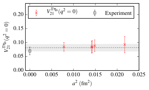
By studying the error budget we see that the main sources of error are from the systematics in . Here, as discussed in Sec. V.2.8, the main sources of uncertainty come from the statistical error in and from not knowing the coefficient of in the expansion of . While the statistical error on could potentially be reduced from to [20], computation of the two-loop coefficient of would be difficult and lengthy, and unlikely to be done in the near future. Alternatively, one could tune against the hyperfine splitting on all ensembles, as shown in Section V.2.9, and the error on could be reduced to .
After this, the main uncertainty comes from the missing currents. These could be included with more computational time if neccessary. While the statistical error on each current alone is around , these statistical errors do not allow the correlations between the data points in the fit to constrain the final result as much as we would like, and the final error from statistics in the error budget is as a result. Reducing the error from statistics is unlikely to have a sizable effect.
Based on our analysis, we estimate that by including the next order of relativistic corrections to the current, the mixing down in , and tuning against the hyperfine splitting on all ensembles, an error on of could be possible (compared against an error of on the value inferred from experiment), where the uncertainties in order of dominance would be from the one-loop corrections to and and the systematic error coming from .
Our final answer for the form factor is:
| (27) |
Final values for the decay rate and branching fraction are given in Section VI.
VI Discussion and Conclusions
In this paper we have computed the hindered M decay rate using a lattice NRQCD formalism for the -quark. We include several improvements on earlier exploratory work [5, 6] which are fundamental to obtaining an accurate value for this decay rate. The key improvements are:
- •
Previous work only had one lattice spacing. We use five ensembles with a fully tadpole-improved Lüscher-Weisz gluon action with HISQ and quarks in the sea, provided by the MILC collaboration. These ensembles each have configurations and one has physical light quark masses.
- •
- •
- •
We calculate the contribution to the matching coefficient of the leading order current which mediates this decay, as described in Section IV.1.
- •
While previous work extracted the matrix element by extrapolating/interpolating to the point, which only gives the photon on-shell contribution if the hyperfine splitting is correct, we use twisted boundary conditions to extract the form factor relevant to this decay at the physical point.
In Section III.5 we performed an analysis of the energy eigenstates of NRQCD at non-zero momentum. This is necessary as the energy eigenstates of a rotationally invariant theory, like NRQCD, in an infinite volume continuum at non-zero momentum are classified by helicity, unlike in a Lorentz invariant theory where they are described by the standard angular momentum . This has important consequences for a lattice NRQCD calculation as additional states appear in the spectrum at non-zero momentum (see Figure 1) and one has to be careful to ensure that the correct matrix elements are extracted from the correlator data.
In Section V, we show results for the four form factors from the currents listed in Section IV which when renormalised, summed and extrapolated to the continuum limit, can be compared to the form factor inferred from experimental data. We found that relativistic corrections to the leading order current gave a negative contribution causing destructive interference, that the power counting of the currents deviated from what one would naively expect in NRQCD, and that a range of sensitivities needed to be explained.
In Section V.2, using a simple potential model, we explained that the matrix element of the leading order current was suppressed due to the orthogonality of the radial wavefunctions, and this causes the matrix element to become sensitive to a multitude of effects such as relativistic corrections to the leading order current, and certain parameters in the NRQCD action that give rise to perturbing potentials causing relativistic corrections to the wavefunctions, particularly those which effect the hyperfine splitting.
It has been suggested [5, 6] that the large changes experienced in going from an unimproved calculation to an improved calculation may mean that it would be beneficial to avoid nonrelativistic approximations. We come to a different conclusion and illustrate that although such a calculation is intrinsically difficult, NRQCD does indeed show that a systematic approach works while also giving insight into the process under study.
After performing the continuum and sea quark mass extrapolation, we obtain the form factor , with a full error budget in Table 14. This form factor can be combined with the experimental masses used in Section II to produce the decay rate:
| (28) |
which can be compared against the experimental decay rate [2, 7]. Using the experimental total width from the PDG average given in Section II with our decay rate gives a branching fraction of which can be compared against the BaBar result of [2]. A comparison of our calculation with potential model results including relativistic corrections [1] is shown in Figure 11.
Potential model predictions of hindered M decay rates are known to be particularly difficult to pin down [38] and can mischaracterise the experimental data by an order of magnitude without relativistic corrections [8]. According to the Quarkonium Working Group reviews [38, 8], sources of uncertainty that contribute to making such decays complicated to calculate include the form of the long range potential chosen, and the results depending explicitly on the quark mass and the perturbative potential chosen. Without relativistic corrections, the branching fraction of the decay from potential model predictions ranges from [1]. Due to the suppression mentioned above, the value of the decay rate is very dependent on good knowledge of the relativistic corrections [1]. Including relativistic corrections, potential model predictions for the same branching fraction have a wider range , showing indeed that the decay rates may be sensitive to small details of the potential [1].
The decay is sensitive to many of the same effects as the hyperfine splitting and an accurate calculation of this decay relies on having the correct hyperfine splitting. Given the large range of estimates of the hyperfine splitting from potential model predictions ( MeV [38]), we should not be surprised that the potential model estimates for this decay rate also have a large range.
Additionally, radiative transitions between bottomonium states provide a search for new-physics effects, seperate from the weak-sector searches common in the literature [47]. For example, the hyperfine splitting between the and has been an important quantity in bottomonium physics, being historically difficult for both experimentalists and theorists to predict reliably. Using hindered M decays, the BaBar [48, 2] and CLEO [49] experiments inferred this hyperfine splitting to be MeV [50]. However, in 2012, BELLE measured the branching fractions (called E decays in the literature), removing the dependence on hindered M decays and used a significantly larger sample of events, to yield a hyperfine splitting of MeV [51], where has a tension with being zero.
It has been suggested that the tension of and theory [16] with could, if it persists, indicate a hint at new physics [52, 53]. For example, in a multiple-Higgs extension to the standard model, one would speculate that the seen in experiments is actually an admixture of the true and a CP-odd Higgs boson with mass ranging from GeV. A relatively light CP-odd Higgs scalar can appear in non-minimal supersymmetric extensions of the standard model, such as the next-to-minimal supersymmetric standard model [53]. In such cases, the measured decay rate for would likely differ from the Standard Model prediction. As stated above, this decay is sensitive in much the same way as the hyperfine splitting. To observe a similar tension between theory and experiment here as that existing between and would require a uncertainty on the form factor ( on the decay rate). The error on the lattice form factor could be reduced to (as discussed in Section V.4) if more precise experimental results became available. Any hint of new physics arising from a deviation between the experimental decay rate and theory could then be explored more concretely. Additionally, the decay is an alternative approach to studying such effects and a study of this decay rate is already underway.
E radiative decays are more easily computed than hindered M decays, and so the E decay rates and could be calculated within this NRQCD framework. Additionally, E currents can be readily renormalised nonperturbatively. Combined with the experimental branching fraction of these decays [51], this could give a prediction of the total width of the and .
ACKNOWLEDGMENTS
We would like to thank Christopher Thomas for the many insightful discussions on the finite-volume lattice inflight spectrum. We are also grateful to the MILC collaboration for the use of their gauge configurations. This work was funded by STFC. The results described here were obtained using the Darwin Supercomputer of the University of Cambridge High Performance Computing Service as part of the DiRAC facility jointly funded by STFC, the Large Facilities Capital Fund of BIS and the Universities of Cambridge and Glasgow.
Appendix A Classification of Particle States
Theoretically, particle states living in the Hilbert space are classified by unitary irreducible representations (irreps) of the symmetry group of a theory. We need to consider two symmetry groups here: the Lorentz group and the continuous rotational group in three dimensions (the symmetry group of NRQCD). The standard procedure to build infinite dimensional unitary irreps of these groups is via the method of induced representations, where one considers finite dimensional unitary irreps of the little group and then uses these to build unitary irreps of the full group.
The Poincaré group is the symmetry group of a relativistic quantum field theory, and is given by the semi-direct product of the Lorentz group and four translations. For massive irreps of the Poincaré group, the little group is 77 7 At nonzero momentum we can perform a Lorentz boost back to the rest frame, ensuring the little group is the same for zero and nonzero three-momentum [54]. Thus in a Lorentz invariant theory, massive irreps are defined as . Note that for quarkonia these states are eigenvectors of the charge-conjugation operator and parity is also a conserved quantum number,88 8 At nonzero momentum, these states are not eigenvectors of the parity operator, but are eigenstates of the operator defined in the text, which conserves parity. giving the standard decomposition. This description classifies experimental states seen to date [7].
In a continuum theory that is only rotationally invariant, the analogue of the Poincaré group is the semi-direct product of the rotational group with the three translations. For a rotationally invariant theory with zero momentum, the little group is also and the states are classified as . Thus states in a rotationally invariant theory at rest overlap with those in a Lorentz invariant theory at rest, where again, parity and charge conjugation are good quantum numbers in similar situations. Given that at nonzero momentum in a rotationally invariant theory we cannot perform a Lorentzian boost to the rest frame, the little group at nonzero momentum is now different to the zero momentum little group. The little group is now 99 9 The construction of the irreps for a rotationally invariant theory at nonzero momentum is similar to a massless representation in a Lorentz invariant theory. [54]. In this case, the unitary irreps are classified by , where is an eigenvalue of the helicity operator . The helicity will get contributions from all with . This can have important consequences for the extracted energy spectrum in NRQCD, c.f., Figure 1 and 2, and is fundamentally different from the Lorentzian theory.
At zero momentum, the operators and that we use in this calculation overlap onto and states in a rotationally invariant continuum theory [26]. We now need to find which helicity eigenstates these operators overlap with at nonzero momentum. The authors of [26] illustrate how to construct helicity operators via
| (29) |
where is a Wigner- matrix, is the active transformation which rotates to , is a helicity operator with helicity in an infinite volume continuum, e.g.,
| (30) |
and we refer the reader to Ref. [26] for further details. For quarkonium, the possibile values of , where the on the represent the symmetry with eigenvalue [26]. Using the fact that the Wigner- matrices with are , the , bilinear operators which we use in this calculation give rise to the helicity operators at nonzero momentum
| (31) |
As can be seen, is a helicity operator which creates a state, but creates an admixture of states.
The question now is: how do we identify which contributes to each , and how do we parameterise the amplitudes? By noticing that the helicity when the momentum is projected onto the -axis, all states with will have a large enough to give a contribution to this helicity state (see Table 3).
We also want to know how to quantify the amplitudes. In a rotationally invariant theory, the invariant quantities are and . For a state, we also have the momentum and the symmetric polarisation tensor . We can use these to parameterise the amplitudes relevant for a rotationally invariant theory. For the operator , Table XI in [26] has the possible decompositions and we reproduce the parameterisations for the operator which are important for our calculation
| (32) | ||||
where is the radial label. Using the overlap for the from (32) to parameterise the continuum two-point correlator with nonzero momentum, one finds that the amplitudes from our fit with local smearing should be suppressed by relative to states which overlap with the operator at zero momentum. For the momentum that we use in our calculation, this factor is around , and we observe that in our correlator data, the amplitudes for the states which do not overlap at zero momentum (and for which we get a signal) such as the , are suppressed by this factor while the other amplitudes are . We observe that as the momentum increases, so does the value of the amplitude at fixed lattice spacing.
Additionally, the symmetry group giving rise to the invariants which classify states, e.g., the little group, is broken by a finite volume lattice to a reduced symmetry group [55]. At zero momentum with a cubic lattice, this reduced symmetry group for quarkonia is the octahedral group, . States are now classified in terms of irreps of , denoted , where [56] shows how to subduce operators with continuum spin to operators with definite on the lattice. As mentioned above, in an infinite-volume continuum theory, the () operator overlaps only with at rest, but this operator falls into the () irrep of on the lattice, where mixing with the state (and higher spins) is possible. However we do not see this mixing: rotational symmetry breaking is found to be weakly broken with a fine lattice and with a rotationally invariant smearing for a particular lattice setup [56], where the spectrum and overlaps were compatible with an effective restoration of rotational symmetry. For this reason, we choose to use a rotationally invariant smearing, an isotropic lattice and have discretisation improvements in our action. Secondly, the masses of the additional states are too large to be seen in the first few energy levels which we are interested in. As such, they will only potentially contribute as additional discretisation effects in the lowest energy modes. Indeed, studies of the spectrum from NRQCD by the HPQCD collaboration indicate this to be the case (see Appendix C of [13]).
For the nonzero momentum case, the reduced little group actually depends on the type of momenta. This is due to the fact that a general integer-valued momentum on the lattice cannot be rotated into the -axis like in an infinite volume continuum, 1010 10 With twisted boundary conditions, the momenta are still discretised but just shifted by an arbitrary value. As such, the little group of momentum with a twist is the same as the little group of momentum without a twist. e.g. there is no octahedral transformation which rotates to the -axis. We use an isotropic momentum (rather than an on-axis momentum) as it has been shown to break rotational invariance less and lead to smaller discretisation effects [13]. For our isotropic momentum, the reduced little group is [26]. The operator () falls into the irrep of , where mixing with states is possible. For , this gives rise to potential mixing from states (and higher spin). As in the zero-momentum case, this mixing due to the lattice was found to be negligible with a fine lattice and a rotationally invariant smearing for a particular setup [26]. These states should be of higher energy than the first few states in our spectrum, and we see no evidence of them in our low lying spectrum. For the operator, there can be mixing with ( with states) which is not important for our analysis.
There is an important distinction to be understood from using a rotationally invariant formalism for the quark versus a Lorentz-invariant one. If each of these formalisms is discretised, then at fixed nonzero momentum, the discretised version of the Lorentz-invariant theory might be broken to a rotationally invariant theory, e.g., by using an anisotropic lattice spacing in the time direction. As such, as the infinite volume continuum limit is taken, any overlap onto as a result of helicity eigenstates (such as the from the operator) would disappear [57]. However, in a rotationally invariant theory like NRQCD, as the lattice spacing is taken to zero, these overlaps are still present as they are an infinite volume continuum effect. This is why we find a similar signal across all lattice spacings for these states in NRQCD.
Appendix B Twisted Correlators with Derivative Operators
For clarity, we will describe the construction of the twisted correlators with derivative operators in this section. To gain access to arbitrary momenta on the lattice, one can define a quark field [22, 23] that satisfies BC via , where . Now the available momentum space is . Notice that the available momentum space has an arbitary shifted value that we can choose to give the physical point . One now builds interpolating operators from these BC fields as , which gives rise to the two-point correlator
| (33) |
where is a quark propagator found by inverting the Dirac matrix, , defined via . As a consequence of satisfying BC, the Dirac matrix also satisfies the same boundary conditions. This is an inconvenience as typical inverters are built with PBC. However, it is possible to use a trick in order to use the PBC invertors yet still get access to the BC correlator data in (33).
To do this, one notices that a second quark field, defined via the scaling , satisfies PBC yet still includes information on the twist. Since
| (34) |
is a quark propagator found by inverting the Dirac matrix, , where . satisfies PBC by construction and the two exponentials only alter the derivative in the Dirac action and can be implemented by scaling the gluonic fields (before inverting) as with [22].
The final step is to rewrite the twisted correlator in (33) in terms of the propagator we actually compute using (34)
| (35) |
If , then
| (36) |
This can be implemented in the same way as the twist in the Dirac invertor, by using in the construction of the covariant derivative operator. This “changing the derivatives” issue does not occur in our two-point correlators, but does occur in the (more complicated) three point correlators with currents , , from (16). To give an explicit example of the three point correlator using the current , by keeping the initial state at rest, and twisting only one propagator in the final state with , we have
| (37) |
where we can clearly see that does not commute with , but not all derivatives are twisted due to the commutation. Since there are no derivatives in the current, the terms cancel and this issue is avoided. Smearing the twisted fields leads to a similar issue as presented above with the derivative, and so we do not smear the twisted fields. Analogous complications arise when using point-split operators with twisted momentum in staggered quark formalisms [58]. If done correctly, and any smearings are applied appropriately, the correlator data from using BC and PBC should agree on a configuration basis to machine precision (if the total momentum is identical for all states).
Appendix C Error Analysis Using a Simple Potential Model
First, we want to find the sensitivity of the matrix element to using a potential from the exchange of a single gluon between two vertices involving the chromomagentic operator [20]. We find (assuming the wavefunctions at the origin for the and are the same)
| (38) |
Putting this back into (22) with the current yields:
| (39) |
In getting to (39) we have used the fact that as the unperturbated Hamiltonian has no spin terms. We have neglected the transitions for in the sum due to the fact that the radial overlap, (20), is suppressed by at least . In fact, they will be suppressed more due to the radial difference getting larger and the wavefunction at the origin getting smaller for higher radial excitations. Eqn. (23) can be found straightforwardly by factoring the spin part of the matrix element from the radial part, i.e., using (20).
If we now consider a potential from the exchange of a single gluon involving the Darwin term at one of the vertices, we find [20]
| (40) |
Then substituting this back into (22) we find:
| (41) |
| (42) |
Using (20), we see the leading order terms in the second piece of (42) cancel and we are left with corrections to the unperturbed matrix element.
The four quark potential is (assuming the wavefunctions at the origin of the two states are the same) [20]
| (43) |
Putting this into (22) and performing an identical analysis as done above gives
| (44) |
The error in the last line was introduced by expanding out the radial overlap (20) and noting that the two matrix elements do not have to be identical to first order in . Even if we did include the four fermion operators in the calculation, since only the combination is currently known perturbatively, and not and individually, we would still need to introduce the error in our calculation.
References
- [1] S. Godfrey and J. L. Rosner, Phys. Rev. D 64, 074011 (2001), arXiv:hep-ph/0104253.
- [2] BaBar, B. Aubert et al., Phys. Rev. Lett. 103, 161801 (2009), arXiv:0903.1124.
- [3] N. Brambilla, Y. Jia, and A. Vairo, Phys. Rev. D 73, 054005 (2006), arXiv:hep-ph/0512369.
- [4] A. Pineda and J. Segovia, Phys. Rev. D 87, 074024 (2013).
- [5] R. Lewis and R. M. Woloshyn, Phys. Rev. D 84, 094501 (2011), arXiv:1108.1137.
- [6] R. Lewis and R. M. Woloshyn, Phys. Rev. D 86, 057501 (2012), arXiv:1207.3825.
- [7] Particle Data Group, K. Olive et al., Chin.Phys. C38, 090001 (2014).
- [8] N. Brambilla et al., Eur.Phys.J. C71, 1534 (2011), arXiv:1010.5827.
- [9] J. J. Dudek, R. G. Edwards, and D. G. Richards, Phys. Rev. D 73, 074507 (2006), arXiv:hep-ph/0601137.
- [10] MILC, A. Bazavov et al., Phys. Rev. D82, 074501 (2010), arXiv:1004.0342.
- [11] HPQCD Collaboration, A. Hart, G. M. von Hippel, and R. R. Horgan, Phys. Rev. D 79, 074008 (2009), arXiv:0812.0503.
- [12] HPQCD Collaboration, UKQCD Collaboration, E. Follana et al., Phys. Rev. D 75, 054502 (2007), arXiv:hep-lat/0610092.
- [13] HPQCD Collaboration, R. J. Dowdall et al., Phys. Rev. D 85, 054509 (2012), arXiv:1110.6887.
- [14] G. P. Lepage, L. Magnea, C. Nakhleh, U. Magnea, and K. Hornbostel, Phys. Rev. D 46, 4052 (1992), arXiv:hep-lat/9205007.
- [15] HPQCD Collaboration, J. O. Daldrop, C. T. H. Davies, and R. J. Dowdall, Phys. Rev. Lett. 108, 102003 (2012), arXiv:1112.2590.
- [16] HPQCD Collaboration, R. J. Dowdall, C. T. H. Davies, T. Hammant, and R. R. Horgan, Phys. Rev. D 89, 031502 (2014), arXiv:1309.5797.
- [17] HPQCD Collaboration, R. J. Dowdall, C. T. H. Davies, T. C. Hammant, and R. R. Horgan, Phys. Rev. D 86, 094510 (2012), arXiv:1207.5149.
- [18] HPQCD Collaboration, R. J. Dowdall, C. T. H. Davies, R. R. Horgan, C. J. Monahan, and J. Shigemitsu, Phys. Rev. Lett. 110, 222003 (2013), arXiv:1302.2644.
- [19] HPQCD Collaboration, B. Colquhoun, R. J. Dowdall, C. T. H. Davies, K. Hornbostel, and G. P. Lepage, Phys. Rev. D 91, 074514 (2015).
- [20] HPQCD Collaboration, T. C. Hammant, A. G. Hart, G. M. von Hippel, R. R. Horgan, and C. J. Monahan, Phys. Rev. D 88, 014505 (2013), arXiv:1303.3234.
- [21] S. Meinel, Phys. Rev. D 82, 114502 (2010), arXiv:1007.3966.
- [22] G. de Divitiis, R. Petronzio, and N. Tantalo, Phys.Lett. B595, 408 (2004), arXiv:hep-lat/0405002.
- [23] D. Guadagnoli, F. Mescia, and S. Simula, Phys. Rev. D 73, 114504 (2006), arXiv:hep-lat/0512020.
- [24] G. P. Lepage, Lsqfit and Corrfitter Python code for Bayesian fitting is available from https://github.com/gplepage/corrfitter.
- [25] G. Lepage et al., Nucl. Phys. Proc. Suppl. 106, 12 (2002), arXiv:hep-lat/0110175.
- [26] C. E. Thomas, R. G. Edwards, and J. J. Dudek, Phys. Rev. D 85, 014507 (2012), arXiv:1107.1930.
- [27] Lattice Hadron Physics, F. D. R. Bonnet, R. G. Edwards, G. T. Fleming, R. Lewis, and D. G. Richards, Phys. Rev. D 72, 054506 (2005), arXiv:hep-lat/0411028.
- [28] HPQCD Collaboration, C. M. Bouchard, G. P. Lepage, C. Monahan, H. Na, and J. Shigemitsu, Phys. Rev. D 90, 054506 (2014), arXiv:1406.2279.
- [29] HPQCD Collaboration, C. McNeile, C. T. H. Davies, E. Follana, K. Hornbostel, and G. P. Lepage, Phys. Rev. D 82, 034512 (2010), arXiv:1004.4285.
- [30] HPQCD Collaboration, K. Hornbostel et al., Phys. Rev. D 85, 031504 (2012), arXiv:1111.1363.
- [31] G. Feinberg and J. Sucher, Phys. Rev. Lett. 35, 1740 (1975).
- [32] J. Sucher, Reports on Progress in Physics 41, 1781 (1978).
- [33] J. S. Kang and J. Sucher, Phys. Rev. D 18, 2698 (1978).
- [34] T. Kinoshita and M. Nio, Phys. Rev. D 53, 4909 (1996).
- [35] A. Hart, G. von Hippel, R. Horgan, and E. Muller, Comput. Phys. Commun. 180, 2698 (2009), arXiv:0904.0375.
- [36] A. Hart, G. von Hippel, R. Horgan, and L. Storoni, J.Comput.Phys. 209, 340 (2005), arXiv:hep-lat/0411026.
- [37] M. A. Nobes, H. D. Trottier, G. P. Lepage, and Q. Mason, Nucl. Phys. Proc. Suppl. 106, 838 (2002), arXiv:hep-lat/0110051.
- [38] Quarkonium Working Group, N. Brambilla et al., (2004), arXiv:hep-ph/0412158.
- [39] R. R. Horgan, private communication.
- [40] HPQCD Collaboration, B. Colquhoun et al., Phys. Rev. D 91, 114509 (2015), arXiv:1503.05762.
- [41] (Fermilab Lattice and MILC Collaborations), A. Bazavov et al., Phys. Rev. D 90, 074509 (2014).
- [42] V. Zambetakis and N. Byers, Phys. Rev. D 28, 2908 (1983).
- [43] H. Grotch, D. A. Owen, and K. J. Sebastian, Phys. Rev. D 30, 1924 (1984).
- [44] S. Godfrey and N. Isgur, Phys. Rev. D 32, 189 (1985).
- [45] X. Zhang, K. J. Sebastian, and H. Grotch, Phys. Rev. D 44, 1606 (1991).
- [46] T. Lahde, C. Nyfalt, and D. Riska, Nuclear Physics A 645, 587603 (1999).
- [47] J. Beringer et al., Phys. Rev. D 86, 010001 (2012).
- [48] BaBar, B. Aubert et al., Phys. Rev. Lett. 101, 071801 (2008), arXiv:0807.1086.
- [49] CLEO, G. Bonvicini et al., Phys. Rev. D 81, 031104 (2010), arXiv:0909.5474.
- [50] Particle Data Group, K. Nakamura et al., J. Phys. G 37, 075021 (2010).
- [51] Belle, R. Mizuk et al., Phys. Rev. Lett. 109, 232002 (2012), arXiv:1205.6351.
- [52] D. Becirevic and F. Sanfilippo, J. High Energy Phys. 1301, 028 (2013), arXiv:1206.1445.
- [53] F. Domingo, U. Ellwanger, and M.-A. Sanchis-Lozano, Phys. Rev. Lett. 103, 111802 (2009), arXiv:0907.0348.
- [54] S. Weinberg, The Quantum Theory of Fields. Vol. 1: Foundations (Cambridge Univ. Pr., 1995).
- [55] D. C. Moore and G. T. Fleming, Phys. Rev. D 73, 014504 (2006), arXiv:hep-lat/0507018.
- [56] J. J. Dudek, R. G. Edwards, M. J. Peardon, D. G. Richards, and C. E. Thomas, Phys. Rev. D 82, 034508 (2010), arXiv:1004.4930.
- [57] Z. Davoudi and M. J. Savage, Phys. Rev. D 86, 054505 (2012), arXiv:1204.4146.
- [58] HPQCD Collaboration, G. C. Donald, C. T. H. Davies, J. Koponen, and G. P. Lepage, Phys. Rev. D 90, 074506 (2014), arXiv:1311.6669.