Empirical Bayesian Analysis of Simultaneous Changepoints in Multiple Data SequencesThanks: ZF was supported by a Hertz Foundation Fellowship and an NDSEG Fellowship (DoD, Air Force Office of Scientific Research, 32 CFR 168a). LM was supported by a Terman Fellowship.
Abstract.
Copy number variations in cancer cells and volatility fluctuations in stock prices are commonly manifested as changepoints occurring at the same positions across related data sequences. We introduce a Bayesian modeling framework, BASIC, that employs a changepoint prior to capture the co-occurrence tendency in data of this type. We design efficient algorithms to sample from and maximize over the BASIC changepoint posterior and develop a Monte Carlo expectation-maximization procedure to select prior hyperparameters in an empirical Bayes fashion. We use the resulting BASIC framework to analyze DNA copy number variations in the NCI-60 cancer cell lines and to identify important events that affected the price volatility of S&P 500 stocks from 2000 to 2009.
1. Introduction
Figure 1 displays three examples of aligned sequence data. Panel (a) presents DNA copy number measurements at sorted genome locations in four human cancer cell lines (Varma et al., 2014). Panel (b) shows the daily stock returns of four U.S. stocks over a period of ten years. Panel (c) traces the interatomic distances between four pairs of atoms in a protein molecule over the course of a computer simulation (Lindorff-Larsen et al., 2011). Each sequence in each panel is reasonably modeled as having a number of discrete “changepoints,” such that the characteristics of the data change abruptly at each changepoint but remain homogeneous between changepoints. In panel (a), these changepoints demarcate the boundaries of DNA stretches with abnormal copy number. In panel (b), changepoints indicate historical events that abruptly impacted the volatility of stock returns. In panel (c), changepoints indicate structural changes in the 3-D conformation of the protein molecule. For each of these examples, it is important to understand when and in which sequences changepoints occur. However, the number and locations of these changepoints are typically not known a priori and must be estimated from the data. The problem of detecting changepoints in sequential data has a rich history in the statistics literature, and we refer the reader to (Basseville and Nikiforov, 1993; Chen and Gupta, 2012) for a more detailed review and further applications.

In many modern applications, we have available not just a single data sequence but rather many related sequences measured at the same locations or time points. These sequences often exhibit changepoints occurring at the same sequential locations. For instance, copy number variations frequently occur at common genomic locations in cancer samples (Pollack and Brown, 1999) and in biologically-related individuals (Zhang et al., 2010), economic and political events can impact the volatility of many stock returns in tandem, and a conformational change in a region of a protein molecule can affect distances between multiple atomic pairs (Fan et al., 2015). As recognized in many recent papers, discussed below, an analysis of multiple sequences jointly may yield greater statistical power in detecting their changepoints than analyses of the sequences individually. In addition, a joint analysis may more precisely identify the times or locations at which changepoints occur and better highlight the locations where changepoints most frequently recur across sequences.
Motivated by these considerations, we introduce a Bayesian modeling framework, BASIC, for carrying out a Bayesian Analysis of SImultaneous Changepoints. In single-sequence applications, Bayesian changepoint detectors have been shown to exhibit favorable performance in comparison with other available methods and have enjoyed widespread use (Chernoff and Zacks, 1964; Yao, 1984; Barry and Hartigan, 1993; Stephens, 1994; Chib, 1998; Fearnhead, 2006; Adams and MacKay, 2007). In Section 2, we propose an extension of Bayesian changepoint detection to the multi-sequence setting by defining a hierarchical prior over latent changepoints, which first specifies the sequential locations at which changepoints may occur and then specifies the sequences that contain a changepoint at each such location.
Inference in the BASIC model is carried out through efficient, tailored Markov chain Monte Carlo (MCMC) procedures (Section 3.1) and optimization procedures (Section 3.2) designed to estimate the posterior probabilities of changepoint events and the maximum-a-posteriori (MAP) changepoint locations, respectively. These procedures employ dynamic programming sub-routines to avoid becoming trapped in local maxima of the posterior distribution. To free the user from pre-specifying prior hyperparameters, we adopt an empirical Bayes approach (Robbins, 1956) to automatic hyperparameter selection using Monte Carlo expectation maximization (MCEM) (Wei and Tanner, 1990) (Section 3.4).
To demonstrate the applicability of our model across different application domains, we use our methods to analyze two different data sets. The first is a set of array comparative genomic hybridization (aCGH) copy number measurements of the NCI-60 cancer cell lines (Varma et al., 2014), four of which have been displayed in Figure 1(a). In Section 5, we use our method to highlight focal copy number variations that are present in multiple cell lines; many of the most prominent variations that we detect are consistent with known or suspected oncogenes and tumor suppressor genes. The second data set consists of the daily returns of 401 U.S. stocks in the S&P 500 index from the year 2000 to 2009, four of which have been displayed in Figure 1(b). In Section 6, we use our method to identify important events in the history of the U.S. stock market over this time period, pertaining to the entire market as well as to individual groups of stocks.
Comparison with existing methods: Early work on changepoint detection for multivariate data (Srivastava and Worsley, 1986; Healy, 1987) studied the detection of a change in the joint distribution of all observed variables. Our viewpoint is instead largely shaped by (Zhang et al., 2010), which formulated the problem as detecting changes in the marginal distributions of subsets of these variables. A variety of methods have been proposed to address variants of this problem, many with a particular focus on analysis of DNA copy number variation. These methods include segmentation procedures using scan statistics (Zhang et al., 2010; Siegmund et al., 2011; Jeng et al., 2013), model-selection penalties (Zhang and Siegmund, 2012; Fan et al., 2015), total-variation denoising (Nowak et al., 2011; Zhou et al., 2013), and other Bayesian models (Dobigeon et al., 2007; Shah et al., 2007; Harlé et al., 2014; Bardwell and Fearnhead, 2017). Here, we briefly highlight several advantages of our present approach.
Comparing modeling assumptions, several methods (Jeng et al., 2013; Bardwell and Fearnhead, 2017) focus on the setting in which each sequence exhibits a baseline behavior, and changepoints demarcate the boundaries of non-overlapping “aberrant regions” that deviate from this baseline. Shah et al. (2007) further assumes a hidden Markov model with a small finite set of possible signal values for each sequence. However, data in many applications are not well-described by these simpler models. For instance, in cancer samples, short focal copy number aberrations may fall inside longer aberrations of entire chromosome arms and overlap in sequential position, and true copy numbers might not belong to a small set of possible values if there are fractional gains and losses due to sample heterogeneity. Conversely, the Bayesian models of (Dobigeon et al., 2007; Harlé et al., 2014) are very general, but their priors and inference procedures involve parameters (where is the number of sequences), rendering inference intractable for applications with many sequences. By introducing a prior that is exchangeable across sequences, we strike a different balance between model generality and tractability of inference.
Comparing algorithmic approaches, we observe in simulation (Section 4) that total-variation denoising can severely overestimate the number of changepoints, rendering them ill-suited for applications in which changepoint-detection accuracy (rather than signal reconstruction error) is of interest. In contrast to recursive segmentation procedures, our algorithms employ sequence-wise local moves, which we believe are better-suited to multi-sequence problems with complex changepoint patterns. These local moves are akin to the penalized likelihood procedure of (Fan et al., 2015), but in contrast to (Fan et al., 2015) where the likelihood penalty shape and magnitude are ad hoc and user-specified, our empirical Bayes approach selects prior hyperparameters automatically using MCEM. Finally, the BASIC approach provides a unified framework that accommodates a broad range of data types and likelihood models, can detect changes of various types (e.g. in variance as well as in mean), and returns posterior probabilities for changepoint events in addition to point estimates.
2. The BASIC Model

Suppose is a collection of aligned data sequences, each consisting of observations.
The BASIC model for is a generative process defined by three inputs: an observation likelihood parameterized by , a prior distribution on the parameter space , and a changepoint frequency prior on .
For each sequence position , a latent variable is
drawn from and represents the probability of any
sequence having a changepoint between its and
data points. Then, for each sequence position and sequence
, a latent variable is drawn with
and indicates whether there is a changepoint in
sequence between its and
data points. Finally, for each
and , a latent likelihood parameter
and an observed data point are drawn, such
that remains constant (as a function of ) in each data
sequence between each pair of consecutive changepoints of that sequence and
is generated anew from the prior at each changepoint, and
is a conditionally independent draw from .
This process is summarized as follows:
The BASIC Model
For notational convenience, we arrange into a matrix , fixing for all . Figure 2 illustrates this generative model in the case where the piecewise-constant parameter represents the mean of the distribution of , and is normally-distributed around this mean with fixed unit variance. Our primary goal in this model will be to infer the latent changepoint variables upon observing the data .
A key input to the model is the prior distribution over , which controls how frequently changepoints occur and to what extent they co-occur across sequences. Rather than requiring the user to pre-specify this prior, Section 3.4 develops an empirical Bayes MCEM procedure to select automatically. Specifically, we parametrize as a mixture distribution
| (1) |
where is a fixed finite dictionary of probability distributions over and are non-negative mixture weights summing to 1, and the MCEM maximum marginal likelihood procedure selects the weights . In our applications, we will simply take the dictionary to be discrete point masses over a fine grid of points in .
The choices of the likelihood model and the prior distribution are application-dependent. For our analysis of DNA copy number variations in Section 5, we use a normal model for where parametrizes the normal mean, and is the normal conjugate prior. For our analysis of stock return volatility in Section 6, we use a Laplace model for with mean 0 and scale parameter , and is the inverse-Gamma conjugate prior. We provide details on these and several other common models in Appendix A. Our inference procedures are tractable whenever the marginal
| (2) |
may be computed quickly from and . This holds, in particular, whenever is an exponential family model with the conjugate prior, as may be computed by updating a fixed number of sufficient statistics. Any unspecified hyperparameters of can also be selected automatically using the MCEM procedure of Section 3.4.
We have assumed for notational convenience that each data sequence is generated from the same parametric family with the same prior . In applications where sequences represent different types of quantities, the choices of and should vary across sequences, and our posterior inference algorithms are easily extended to accommodate this setting.
3. Inference procedures
In this section, we give a high-level overview of our algorithms for posterior inference in the BASIC model, deferring details to Appendices B-D. Our primary task is to perform posterior inference of the unobserved latent changepoint variables , given the observed data . Assuming and are fixed and known, Section 3.1 presents an MCMC procedure for sampling from the posterior distribution , and Section 3.2 presents an optimization algorithm to locally maximize this posterior distribution over to yield a MAP estimate. Section 3.4 presents an MCEM method to select and , following the empirical Bayesian principle of maximum marginal likelihood. An efficient implementation of all inference algorithms is available on the authors’ websites.
We emphasize that even though the BASIC model is specified hierarchically, our inference algorithms directly sample from and maximize over the posterior distribution of only , analytically marginalizing over the other latent variables and . Furthermore, these procedures use dynamic programming subroutines that exactly sample from and maximize over the joint conditional distribution of many or all variables in a single row or column of , i.e. changepoints in a single sequence or at a single location across all sequences. We verify in Appendix E that this greatly improves mixing of the sampler over a naïve Gibbs sampling scheme that individually samples each from its univariate conditional distribution.
3.1. Sampling from the posterior distribution
To sample from , we propose the following high-level MCMC procedure:
- (1)
For : Re-sample from
- (2)
For : Re-sample from
- (3)
For : Randomly select such that for at least one , choose or , and perform a Metropolis-Hastings step to swap and .
We treat the combination of steps 1–3 above as one complete iteration of our MCMC sampler. Here, , , , and respectively denote the row, all but the row, the column, and all but the column of . In step 3, is the number of swap attempts, which we set in practice as .
To sample in step 1, we adapt the dynamic programming recursions developed in (Fearnhead, 2006) to our setting, which require time for each . To sample in step 2, we develop a novel dynamic programming recursion which performs this sampling in time for each . Step 3 is included to improve the positional accuracy of detected changepoints, and the swapping of columns of typically amounts to shifting all changepoints at position to a new position or that previously had no changepoints. This step may be performed in time (when ), so one complete iteration of steps 1–3 may be performed in time . Details of all three algorithmic procedures are provided in Appendix B.
3.2. Maximizing the posterior distribution
To maximize over , we similarly propose iterating the following three high-level steps:
- (1)
For : Maximize over .
- (2)
For : Maximize over .
- (3)
For each such that for at least one , swap with or if this increases , and repeat.
We terminate the procedure when one iteration of all three steps leaves unchanged. In applications, we first perform MCMC sampling to select and using the MCEM procedure to be described in Section 3.4, and then initialize in the above algorithm to a rounded average of the sampled values. Under this initialization, we find empirically that the above algorithm converges in very few iterations.
To maximize over in step 1, we adapt the dynamic programming recursions developed in (Jackson et al., 2005) to our setting, which require time for each . Maximization over in step 2 is easy to perform in time for each . Step 3 is again included to improve the positional accuracy of detected changepoints, and after an initialization, each swap of step 3 may be performed in time. Hence one complete iteration of steps 1–3 may be performed in time . Details of all three algorithmic procedures are provided in Appendix C.
3.3. Reduction to linear cost in
In practice, may be large, and it is desirable to improve upon the quadratic computational cost in . For sampling, one may use the particle filter approach of (Fearnhead and Liu, 2007) in place of the exact sampling procedure in step 1, adding a Metropolis-Hastings rejection step in the particle-MCMC framework of (Andrieu et al., 2010) to correct for the approximation error. For maximization, one may use the PELT idea of (Killick et al., 2012) to prune the computation in step 1, with modifications for a position-dependent cost as described in (Fan et al., 2015).
In our applications we adopt a simpler approach of dividing each row into contiguous blocks and sampling or maximizing over the blocks sequentially; details of this algorithmic modification are provided in Appendices B–C. This reduces the computational cost of one iteration of MCMC sampling to and of one iteration of posterior maximization to , provided the block sizes are . In all of our simulated and real data examples, we use a block size of 50 data points per sequence. We examine the effect of block size choice in Appendix E.
3.4. Empirical Bayes selection of priors and
To select and automatically using the empirical Bayes principle of maximum marginal likelihood, we assume is a mixture as in Eq. 1 over a fixed dictionary , and we estimate the weights . We also assume that is parametrized by a low-dimensional parameter , and we estimate . We denote in Eq. 2 by .
Let denote the data segments induced by changepoints , i.e., and for all other . Let be the total number of positions where exactly sequences have a changepoint. Our MCEM approach to maximizing the marginal likelihood over candidate priors operates on the “complete” marginal log-likelihood,
Starting with the initializations and , EM iteratively computes the expected complete marginal log-likelihood (E-step)
and maximizes this quantity to select new prior estimates (M-step)
MCEM approximates the E-step by a Monte Carlo sample average,
where are MCMC samples under the prior estimates and . Maximization over and are decoupled in the M-step:
where . Maximization over is convex, and we use a tailored KL-divergence-minimization algorithm for this purpose. We use a generic optimization routine to maximize over the low-dimensional parameter . In our applications, we take to be point masses at a grid of points with spacing and spanning the range , and we initialize to assign large weight at 0 and spread the remaining weight uniformly over the other grid points. We initialize by dividing the data sequences into blocks and matching moments. Details of the optimization and initialization procedures are given in Appendix D.
4. Simulation studies
4.1. Assessing inference on a small example
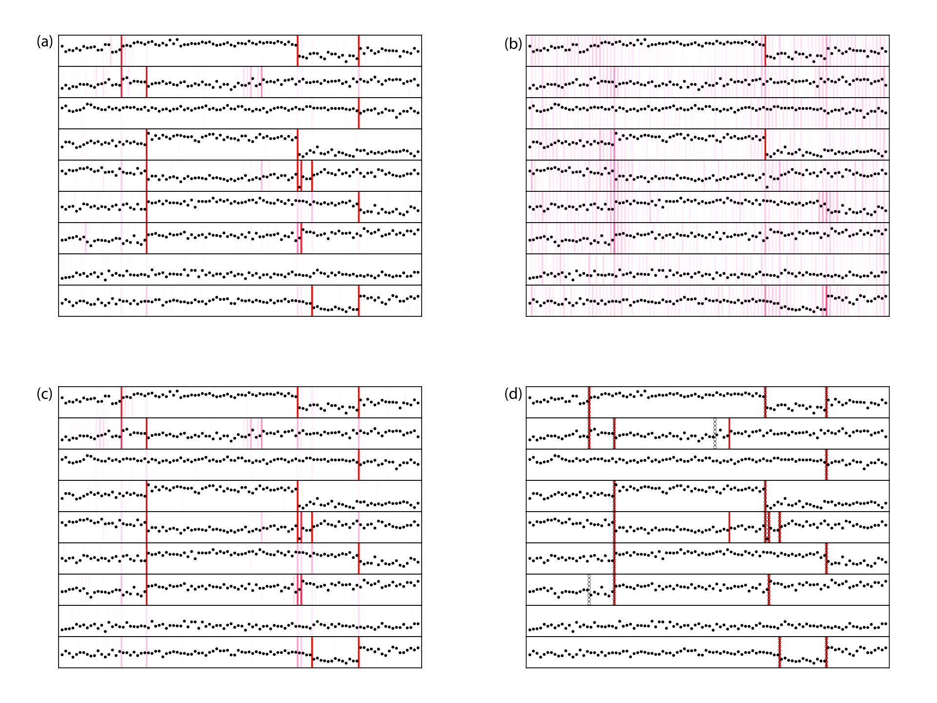
We first illustrate our inference procedures on the small data example shown in Figure 2, with sequences and data points per sequence. This data was generated according to the BASIC model (with , , given by and , and ).
Figure 3 shows the effectiveness of the empirical Bayesian MCEM approach to inference in this setting. Panel (a) shows the marginal posterior changepoint probabilities computed with 50 MCMC samples after a 50-sample burn-in, in an idealized setting where the sampling is performed under the true priors and that generated the data. The results of panel (a) represent an idealized gold standard, as “true priors” are typically unknown in practice. Panel (c) demonstrates, however, that performance comparable to the gold standard can be obtained using MCEM-selected priors, even when the MCEM algorithm is initialized with a grossly incorrect prior guess. In particular, panel (b) displays under the grossly incorrect prior choices , , and , while panel (c) displays when prior parameters are initialized to the same grossly incorrect choices and updated with an MCEM update after iterations 5, 10, 20, 30, and 50 of the burn-in. Notably, the posterior inferences using MCEM priors (panel (c)) are comparable to those of the idealized setting (panel (a)), despite this incorrect initialization. Finally, panel (d) shows the MAP estimate of using the priors estimated in panel (c). In this example, the MAP estimate misses two true changepoints and makes two spurious detections.
We repeated this simulation with 100 different data sets generated from the BASIC model. Table 1 summarizes results using three error measures (all averaged across the 100 experiments): the squared error of the posterior mean changepoint indicators , the squared error of the posterior mean signal reconstruction , and the 0–1 error of detected changepoints in the MAP estimate. All evaluation metrics indicate that posterior inference using the MCEM-selected prior consistently leads to accuracy comparable to the idealized gold standard of using the true data-generating prior. As a reference point for the difficulty of this simulated data, the average 0–1 changepoint error of applying a univariate changepoint method (PELT with default MBIC penalty in the “changepoint” R package, Killick et al. (2012)) to each data sequence individually is 12.6, which is 25% higher than that of our MAP estimate under the MCEM-selected prior.
| True priors | Wrong priors | MCEM priors | |
|---|---|---|---|
| Squared error of | 8.1 | 17.9 | 8.3 |
| Squared error of | 50.3 | 151 | 51.1 |
| 0–1 changepoint error of | 10.3 | 14.9 | 10.1 |
4.2. Comparing detection accuracy on artificial CNV data
The identification of copy number variations (CNVs) in aCGH data for cancer cells represents one primary motivation for our work. As there is typically no known “gold standard” for the locations of all CNVs in real aCGH data, we will assess changepoint detection accuracy in a simulation study, applying our inference procedures to 50 simulated aCGH data sequences using the simulator from Louhimo et al. (2012)11 1 This simulator also generates corresponding gene expression data; we ignored this additional data, as integration of these two data types is not the focus of our paper.. This simulator generates six CNVs that are either focal high-level (2-copy loss or 6-to-8-copy gain), focal medium-level (1-copy loss or 4-copy gain), or broad low-level (1-copy gain). The prevalence of each CNV across samples ranges between 5% and 50%. The simulator accounts for sample heterogeneity, with each sample corresponding to a random mixture of normal and abnormal cells.
Signal reconstruction error
| Method | |
|---|---|
| BASIC | 10.40 |
| SIMPLE | 10.42 |
| CBS | 21.82 |
| cghseg | 29.23 |
| TVSp | 54.22 |
To apply BASIC, we performed 100 iterations of MCMC sampling after 100 iterations of burn-in, using a normal likelihood model with changing mean and fixed (unknown) variance, and with MCEM updates of prior parameters after iterations 10, 20, 40, 60, and 100 of the burn-in. We then performed MAP estimation using the resulting empirical Bayes priors, with initialized to the MCMC sample average. On this data, the BASIC MAP estimate achieved 100% accuracy; we report results in Appendix F.
One way in which this synthetic data is easier than the real aCGH data we analyze in Section 5 is that focal and broad CNVs span at least 50 and 500 probes, respectively, whereas they are shorter in our data of Section 5 and also in certain previous single-sample comparison studies (Lai et al., 2005). To increase the difficulty in this regard, we subsampled every tenth point of each synthetic data sequence and analyzed the resulting sequences, in which focal CNVs span 5 probes and broad CNVs span 50. Results on this more challenging dataset are reported here.
The accuracy of the BASIC MAP estimate is shown as the red star in Figure 4, where we plot the fraction of true changepoints discovered against the false-discovery proportion. Shown also in Figure 4 are the results of several alternative methods: SIMPLE (Fan et al., 2015) to represent the penalized likelihood approach, TVSp (Zhou et al., 2013) to represent total-variation regularization, circular binary segmentation (CBS) (Olshen et al., 2004) applied separately to each sequence to represent a popular method of unpooled analysis, and cghseg (Picard et al., 2011) to represent a popular method of pooled analysis. We set the convergence tolerance of TVSp to and ignored changes with mean shift less than to avoid identifying breakpoints because of numerical inaccuracy. We applied SIMPLE with a normal likelihood model; as the method does not prescribe a default value for the main tuning parameter, we plot its performance as the tuning parameter varies. All remaining parameters of the methods were set to their default values or selected using the provided cross-validation routines.
Detection accuracy of the BASIC MAP estimate is near-perfect and competitive with the other tested methods—examination of its output reveals that it misses a focal (5-probe) medium-level loss in two sequences and a broad low-level gain in one sequence, and it makes one spurious segmentation in one sequence. Detection by cghseg is conservative, missing 10 focal gains and losses across all sequences. In addition, as cghseg does not attempt to identify changepoints at common sequential positions, it inaccurately identifies the location of 15 additional changepoints, which contributes both to an increased false discovery proportion and a reduced true discovery proportion. (This positional inaccuracy ranges between 1 and 5 probes.) Single-sequence CBS suffers from the same changepoint location inaccuracy. It is less conservative than cghseg, truly missing only 3 aberrations across all sequences, but also identifying 2 non-existent aberrations. TVSp partitions the data sequence into too many segments, yielding false-discovery proportion close to 1 for changepoint discovery. We do note that TVSp and its tuning-parameter selection procedure are designed to minimize the signal-reconstruction squared error, rather than changepoint identification error. However, we report the signal reconstruction errors alongside Figure 4 and observe that TVSp is also less accurate by this metric.
SIMPLE yields performance close to that of BASIC under optimal tuning, but the authors of (Fan et al., 2015) provide little guidance on how to choose the tuning parameter. In the BASIC framework, the analogous hyperparameters of are selected automatically by MCEM.
5. Copy number aberrations in the NCI-60 cancer cell lines
We applied our BASIC model to analyze CNVs in aCGH data for the NCI-60 cell lines, a set of 60 cancer cell lines derived from human tumors in a variety of tissues and organs, as reported in (Varma et al., 2014). We discarded measurements on the sex chromosomes, removed outlier measurements, and centered each sequence to have median 0; we discuss these preprocessing steps in Appendix G. We fit the BASIC model using a normal likelihood with changing mean and fixed variance, applying the same procedure as in Section 4.2. The runtime of our analysis on the pooled data () was 2 hours.
In this data, measurements for 59 of the 60 cell lines were made with at least two technical replicates. We used this to test the changepoint detection consistency of various methods, by constructing two data sets of 59 sequences corresponding to the two replicates and applying each method to the data sets independently. A detected changepoint is “coincident” across replicates if it is also detected in the same cell line at the same probe location in the other replicate. Figure 5 plots the total number of coincident detections versus the fraction of all changepoint detections that are coincident, for the methods tested in Section 4.2. (We omit the comparison with TVSp due to its high false-discovery rate for changepoint identification.) BASIC has better performance than single-sample CBS, yielding more coincident detections also at a higher coincidence rate. BASIC is less conservative than cghseg, detecting more coincident changes but at a lower coincidence rate. Recall that the performance of SIMPLE varies with its unspecified tuning parameter. For comparable tunings of SIMPLE, BASIC yields slightly better performance: for the same level of changepoint coincidence across replicates, BASIC detects more changepoints, and for comparable numbers of detected changepoints, BASIC achieves a higher level of changepoint coincidence.
We emphasize that a non-coincident detection is not necessarily wrong—for a changepoint demarcating a low-level aberration against which a method does not have full detection power, a method may detect this change in one replicate but not the other. Conversely, a coincident detection need not correspond to a true CNV, if technical artifacts are present in both replicates. The coincidence rate is not high for any tested method. Reasons for this include (1) changepoints due to technical drift, a common occurrence (Olshen et al., 2004) which is particularly severe in some of the sequences of this data set; (2) probe artifacts that differ across replicates; and (3) low-level non-shared aberrations with boundary points that are difficult to precisely identify. The coincidence rate may be increased for all methods by applying post-processing procedures to remove changepoints due to technical drift and probe artifacts, although these procedures are usually ad hoc.

Our BASIC framework provides not only a point estimate of changepoints, but also posterior probability estimates that may be valuable in interpreting results and also performing this type of post-processing. Figure 6 displays the -ratio measurements and the BASIC MAP estimate of changepoints in chromosome 1 for four distinct melanoma cell lines, alongside the estimated marginal posterior changepoint probabilities. Figure 6 also displays the posterior mean estimate of (computed from the sampled matrices), which provides a cross-sample summary of the prevalence of shared changepoints across all analyzed sequences at each probe location.

To illustrate one use of this posterior information, we performed a pooled analysis of all sequences (including all replicates to increase detection power and accuracy) in order to highlight genomic locations that contain focal and shared CNVs. First, we identified all pairs of genomic locations and on the same chromosome at distance less than base pairs apart22 2 We use 3 million base pairs as the cut-off to distinguish focal from non-focal CNVs. such that at least two distinct cell lines had posterior probability greater than 90% of containing changepoints at both and . The interval between and is the identified CNV, and the sequences having posterior probability greater than 90% of change at and are the identified carriers of that CNV. To reduce false discoveries due to technical noise of the aCGH experiments, we restricted attention to those pairs for which this interval contained at least three microarray probes. Then, for each such pair, we computed the mean value of the data in the interval between and for the carrier sequences and compared this to the mean value in small intervals before and after . Figure 7 shows the 20 identified CNVs that exhibit the greatest absolute difference between these mean values, displaying up to five distinct carriers of each CNV. CNVs that overlap in genomic position are grouped together in the figure.
Many of the CNVs highlighted in Figure 7 contain genes that have been previously studied in relation to cancer; we have annotated the figure with some of these gene names. CDKN2A and CDKN2B are well-known tumor suppressor genes whose deletion and mutation have been observed across many cancer types (Kamb et al., 1994; Nobori, 1994). FBXW7 is a known tumor suppressor gene that plays a role in cellular division (Akhoondi et al., 2007). MYC is a well-known oncogene that is commonly amplified in many cancers (Dang, 2012). URI1 is a known oncogene in ovarian cancer (Theurillat et al., 2011). FAF1 is believed to be a tumor suppressor gene involved in the regulation of apoptosis (Menges et al., 2009). Deletion of A2BP1 has been previously observed in colon cancer tumors and gastric cancer cell lines (Trautmann et al., 2006; Tada et al., 2010). Deletion of APOBEC3 has been observed in breast cancer (Long et al., 2013; Xuan et al., 2013), although we detect its deletion in cell lines of cancers of the central nervous system and the lung. Deletion of CFHR3 and CFHR1 is not specifically linked to cancer, but it is a common haplotype that has been observed in many healthy individuals (Hughes et al., 2006). Many of the remaining CNVs in Figure 7 appear to represent true copy number variations present in the data (rather than spurious detections by our algorithm), but we could not validate the genes present in the corresponding genomic regions against the cancer genomics literature.
6. Price volatility in S&P 500 stocks

As a second example, we applied the BASIC model to analyze the volatility in returns of U.S. stocks from the year 2000 to 2009. We collected from Yahoo Finance the daily adjusted closing prices of stocks that were in the S&P 500 index fund over the entire duration of this 10-year period, and we computed the daily return of each stock on each trading day as , where is its closing price on day and is its closing price on the previous day. Our data consists of the returns for stocks over trading days, and the total runtime of our pooled analysis was 1 hour.
Previous authors have applied univariate changepoint detection methods to analyze daily returns of the Dow Jones Industrial Index from 1970 to 1972, modeling the data as normally distributed with zero mean and piecewise constant variance (Hsu, 1977; Adams and MacKay, 2007). We observed empirically for our data that the tails of the distribution of daily returns are heavier than normal, and we instead applied BASIC using a Laplace likelihood with fixed zero mean and piecewise constant scale. We used the same MCMC/MCEM/MAP inference procedure as in Section 4.2.
Shown in Figure 8 are the daily returns for American International Group Inc. (AIG), Aon Corp. (AON), Bank of America Corp. (BAC), and The Bank of New York Mellon Corp. (BK), together with MAP changepoint estimates and estimated marginal posterior change probabilities. Shown also is the cross-sample changepoint summary provided by the posterior mean of . Within this 10-year period, the 15 trading days with the highest posterior mean for are, in chronological order: Sep 6 2001, Sep 17 2001, Jun 27 2002, Jul 1 2002, Aug 9 2002, Sept 24 2002, Nov 29 2002, Jul 24 2007, Aug 20 2007, Sep 15 2008, Sep 29 2008, Dec 9 2008, Jun 2 2009, Jun 3 2009, and Nov 10 2009. The changepoints from 2001 to 2002 are attributable to the collapse of the dot-com bubble of the late 1990s and early 2000s, and those from 2007 to 2009 are attributable to the U.S. financial crisis. Several of these dates correspond to important events in U.S. stock market history, including Sep 17 2001 when the markets first re-opened after the World Trade Center terrorist attacks, Jul 1 2002 when WorldCom stock fell in value by 93%, Sept 15 2008 when Lehman Brothers filed for Chapter 11 bankruptcy, and Sept 29 2008 when the U.S. House of Representatives rejected a proposed bailout plan for the financial crisis.
Many other detected changepoints were local to small numbers of individual stocks. For instance, the changepoint detected on Oct 14 2004 and visible in the first two sequences of Figure 8 was shared across the seven stocks AIG, AON, Coventry Health Care, Hartford Financial Services, Marsh & McLennan, Merk & Co., and Unum Group. Six of these seven stocks belong to the insurance industry, and the changepoint represents a brief spike in price volatility due to an insurance scandal that was revealed on Oct 14 2004 when AIG publicly disclosed its involvement, along with Marsh & McLennan and others, in an illegal market division scheme, and civil and criminal charges were announced against Marsh & McLennan and employees at AIG pertaining to various allegations of corporate misbehavior.33 3 Source: “Just how rotten?”, The Economist, Special Report, 21 October 2004. Other examples of detected “locally-shared” changepoints include Oct 10 2000, marking the beginning of a period of increased price volatility in the tech companies Amazon.com, Cisco Systems, EMC Corporation, JSD Uniphase, Oracle Corporation, and Yahoo! Inc.; and Feb 16 2005, coinciding with the date on which the international Kyoto Protocol treaty on carbon emissions took effect and marking the start of a period of increased price volatility in the energy companies Dominion Resources, Devon Energy, Public Service Enterprise Group, and Exxon Mobil.
We may also use our methods to produce a smooth estimate of the historical volatility of stock prices, by computing the posterior mean of the Laplace scale parameter for each sequence and each day using the sampled matrices. The Laplace scale parameter implies a standard deviation of ; red lines in Figure 8 are plotted at standard deviations to pictorially illustrate this volatility estimate. This estimate is smooth and resilient to outliers, while still exhibiting rapid adjustments to real structural changes in the data.
Appendix A Likelihood models
For concreteness, we record here several practically-relevant choices of and
in the BASIC model, along with the corresponding computations for in
Eq. 2. In each of these
settings, the prior distribution is parametric, and we denote the
parameter of as .
Normal model, changing mean and fixed variance:
| (3) | ||||
Normal model, changing variance and fixed mean:
| (4) | ||||
Normal model, changing mean and variance:
| (5) | ||||
Poisson model, changing mean:
| (6) | ||||
Bernoulli model, changing success probability:
| (7) | ||||
Laplace model, changing scale and fixed zero mean:
| (8) | ||||
Appendix B MCMC sampling algorithms
Below are the details of the MCMC sampling steps discussed in Section 3.1. Throughout, we define the quantities
| (9) | ||||
| (10) |
for in Eq. 9 and in Eq. 10.
These quantities depend only on and may be pre-computed
outside of the sampling iterations.
(If is discrete or a mixture of Beta distributions, these quantities
are easily computed analytically. Otherwise, these may be computed numerically
for each .) The computational costs of our MCMC sampling and MAP estimation
procedures depend on only via pre-computation of and .
Step 1: Gibbs sampling by rows
To sample each row conditional on the remaining rows , we may employ the dynamic programming recursions developed by Paul Fearnhead for the univariate changepoint problem (Fearnhead, 2006), in the following manner.
Let denote the number of changepoints at position in all but the sequence, and let denote probability conditional on , with associated conditional expectation . Note that is deterministic under . Then the probability density function of conditional on is given, for each , by
Letting , this implies that
| (11) |
For each , let , and let . is the joint probability density of the observed data in sequence after and including position , conditional on a changepoint having occurred in sequence at position and also conditional on the observed changepoints in all of the other sequences. Let be as defined in Eq. 2. Then satisfies the following recursions, which are similar to those in Theorem 1 of (Fearnhead, 2006):
| (12) | ||||
| (13) |
Eq. 13 holds also for , by the same derivation. Eqs. 12 and 13 allow us to compute for recursively via a “backward pass”. We may then sample each successive location where , conditional on the data and , in a “forward pass”:
| (14) | ||||
| (15) |
To summarize, the procedure to sample is as follows:
- (1)
For each , compute according to Eq. 11.
- (2)
- (3)
Regarding computational cost, let us assume that may be updated from in constant time, as is true for all of the parametric models in Eqs. 3–8. Then computing the value of for in step (1) above takes time. For step (2), the value of the summand for each in Eq. 13 may be updated from that for in constant time, so each may be computed in time, and step (2) may be performed in time. Finally, the value in the numerator of Eqs. 14 and 15 for each may be updated from that for in constant time, so step (3) may be performed in time. Hence, sampling for all sequences may be performed in time.
We next describe the modification of this sampling algorithm to sample each row in a block-wise fashion, by dividing each row into blocks and Gibbs sampling the blocks sequentially. Let , and let , with the conventions if and if . Let denote probability conditional on , , and . (Note then that and are deterministic under .) Let for , and . Then, in the backward pass, we may compute
and sample each successive location where , for , by
The derivations of these expressions are similar to those for Eqs. 12–15, and we omit them for brevity.
The time required to sample each block of
changepoint variables is , reducing
the time required to sample all blocks of to if the block
sizes are . Then the total computational cost of sampling
for all sequences is reduced from
to .
Step 2: Gibbs sampling by columns
To sample each column conditional on the remaining columns , let and denote the changepoints in the sequence immediately before and after time , i.e., and , with the conventions if and if . Let denote probability conditional on with associated conditional expectation . Note that and are deterministic under . Let
| (16) | ||||
| (17) |
for each , where is as defined in Eq. 2. For each and each , let be the coefficient of in the polynomial , with the convention . We may compute all of the values recursively for in an “upward pass”:
| (18) | ||||
| (19) |
Let denote the number of changepoints at position in sequences 1 to , with . Then
Letting , this implies
| (20) |
where and are as in Eqs. 9–10. We may then sequentially sample , conditional on the data and , in a “downward pass”:
| (21) |
To summarize, the procedure to sample is as follows:
- (1)
- (2)
- (3)
Regarding computational cost, computation of and for in step (1) requires time if we compute the values of and by updating them from and . In step (2), computation of for and may be performed in time. In step (3), computation of for a single value of may be performed in time, so step (3) may also be performed in time. Hence, sampling for all positions may be performed in time.
A computational shortcut is provided by noting that the
sums in the numerator and denominator of Eq. 20 typically decay rapidly
as increases;
this is theoretically justified by the fact that for each and ,
is a log-concave sequence (being the coefficients of a
real polynomial with real roots, see Theorem 2 of (Stanley, 1989)) and that the
mode of this sequence occurs near if most sequences do not
provide evidence of a changepoint at position . Hence in practice we
truncate these sums in step (3) when the size of the summand falls
below a small threshold, and we compute and store the values in
step (2) via lazy evaluation, only as they are needed in step (3). We
observe empirically that this yields a very significant reduction in
computational time and does not affect the results of posterior inference.
Step 3: Swapping columns by Metropolis-Hastings
Let be as defined in Eq. 2. The following describes a Metropolis-Hastings move that potentially swaps two adjacent columns of the changepoint variable matrix :
- (1)
Let be the set of positions where there is at least one changepoint. Select uniformly at random from , and set or randomly with probability each. If , set with probability 1, and if , set with probability 1. (Recall that in our notation, is fixed for .)
- (2)
For each , if , let , and let , with the conventions if and if . Compute
- (3)
If , or if , then swap and with probability . If and , then swap and with probability . Finally, if and , then swap and with probability .
To see that this procedure keeps the posterior distribution invariant, let denote with columns and swapped. Note that under the BASIC model, . Then the quantity computed in step (2) above is precisely
The procedure of selecting in step (1) induces a transition probability , where in most cases, with the exceptions and if and or , and and if and or . Step (3) above handles all cases with the correct Metropolis-Hastings acceptance probability. In practice, the most common scenario is when there are no changepoints at position , in which case the “swap” of columns and simply shifts all changepoints at position by one position.
Regarding computational cost, to perform the above procedure, one may precompute for each sequence and each pair of consecutive changepoints in sequence (i.e., , , and ). This requires computational cost. Then step (1) above requires cost, step (2) requires cost, and step (3) requires cost. Upon performing the swap in step (3), the set and the values may easily be updated in time, to prepare for the next application of this Metropolis-Hastings move. Hence, performing total iterations of the Metropolis-Hastings move requires time. In our applications we set , and we observe that the computational cost of performing all Metropolis-Hastings steps is much smaller than the cost of the row-wise and column-wise Gibbs sampling procedures.
Appendix C Posterior maximization algorithms
Below are the details of the iterative posterior maximization algorithm
discussed in Section 3.2.
Step 1: Maximizing over rows
Note that , so maximizing over the row is equivalent to maximizing . To perform this maximization, we may employ the dynamic programming recursions developed by Brad Jackson et al. for the univariate changepoint problem (Jackson et al., 2005), in the following way.
Note that
| (22) |
where may be computed as Eq. 11. Define , the marginal probability density of the first data point in sequence assuming there is a changepoint immediately after it, and for , define
Then Eq. 22 is exactly , and we wish to compute the sequence that achieves the maximal value . We do this by iteratively computing for .
Let be the value of if there are no changepoints before position in sequence , and for , let
be the maximal value of assuming that the last changepoint in sequence before position occurs at position . Then, with as in Eq. 2,
| (23) | ||||
| (24) | ||||
| (25) | ||||
| (26) |
The above recursions are similar to those in Section II of (Jackson et al., 2005). From these recursions, we may compute for each by computing for each . In the sequence that achieves the maximum value , the last changepoint is the index such that , the changepoint before is the index such that , etc.
To summarize, the procedure to maximize over is as follows:
- (1)
For each , compute according to Eq. 11.
- (2)
- (3)
Let . While the smallest value in is greater than 1, let this smallest value be , let be the value that achieved , update , and repeat. When the smallest value in becomes 1, set for each with , and set for all other .
Regarding the computational cost, computation of for in step (1) above requires time. For step (2), may be computed in time for each , and may be updated from in constant time for each , so all of the values and for and in step (2) may be computed in time. Since step (3) may be performed in time, maximizing over for all may be performed in time.
We next describe the modification of this maximization algorithm to maximize over each row in a block-wise fashion, by dividing each row into blocks and maximizing over the blocks sequentially. Let , and let , with the conventions if and if . Then we may set and compute recursively for and
The interpretations and derivations of the above expressions are similar to those for Eqs. 22–26, and we omit them for brevity. Then, initializing , we may iteratively take the smallest value in , let be such that , update , and repeat until , to obtain that maximizes the posterior probability over this block.
The time required to maximize over each
block is ,
reducing the time required to maximize over all blocks of to
if the block sizes are . Then the total computational cost of
maximizing over for all sequences is reduced
from to .
Step 2: Maximizing over columns
Note that , so maximizing over the column is equivalent to maximizing . To perform this maximization, let denote the number of changepoints at position . Note that is a function of . Let and denote the changepoints in the sequence immediately before and after position , i.e., and , with the conventions if and if . Recall the quantities and from Eqs. 16 and 17. Then
where is defined in Eq. 9. For any fixed , the above quantity is maximized by setting for the indices that correspond to the largest values of , and setting for all other . Hence, to maximize over , we may perform the following procedure:
- (1)
- (2)
For each , compute the maximum value of over such that . Let be the value of that maximizes this value.
- (3)
Set for the values of corresponding to the largest values of , and set for all other .
Regarding computation cost,
may be computed for in step (1) in
time, if and are updated from and ,
and they may be sorted in time. Step (2)
may be performed in time. Since step (3) also may be performed in
time, maximizing over
for all may be performed in time.
Step 3: Swapping columns
The following procedure allows for adjustment of all changepoints at a position to a new position or : Let be the set of positions where there is at least one changepoint. For , let denote with columns and swapped, and let denote with columns and swapped. While there exists such that is less than or , update to or accordingly, and repeat. Note that as and , the posterior probability always increases with each swap. As in the case of our Metropolis-Hastings move in Section 3.1, the primary purpose of this routine is to swap column for column or when , in which case the “swap” simply moves all changepoints at position to .
Regarding computational cost, one may precompute for each sequence and each pair of consecutive changepoints in sequence . This requires computational time where is the total number of positions with a changepoint in . Then it is evident that and may be computed in time from these quantities. Upon performing a swap of, say, with , the new values and for changepoints immediately preceding and following may be computed in time, to prepare for evaluation of the next swap. Hence each swap throughout the procedure may be performed in time. In practice, we observe that very few swaps are made, and the total computational cost of column-swapping is dominated by the initialization time and is also negligible compared to the costs of row-wise and column-wise maximization over .
Appendix D MCEM algorithms
We describe details of the maximization steps in our MCEM procedure. Maximization over is dependent on the choices of the likelihood model and the prior model . In all of the examples of Eqs. 3–8, is a low-dimensional parameter, and a closed-form expression is available for computing . We use the BOBYQA zeroth-order optimization routine (Powell, 2009), as implemented in the C++ dlib library, to maximize over .
For the maximization over the probability weights , observe that the objective function is a convex function of these weights. In fact, define a probability measure on by
i.e. is the probability under of observing exactly changepoints at any position . Denote by the distribution over with mass function . (Note that by definition of , so .) Then the cross entropy between and is given by
As this cross entropy is equal to , where denotes the Kullback-Leibler divergence and denotes the Shannon entropy, this implies
for a constant independent of . Hence the optimization over may be written as
| (27) |
This may be solved efficiently via an iterative divergence minimization procedure
| (28) |
which converges to the global optimum in Eq. 27, provided that it is initialized to a probability vector supported on all of (Csiszár and Shields, 2004; Lashkari and Golland, 2007). To iteratively compute the update in Eq. 28, one may precompute for each and .
In our applications, we take , and we initialize such that and the remaining probability mass of 0.1 is spread equally over the other grid points . We initialize by dividing the data in each sequence into blocks of 100 data points, computing the sample mean and/or variance within each block, and matching the empirical moments of these sample means and/or variances to their theoretical moments under the prior . For instance, for the normal model with changing mean, Eq. 3, we initialize to the empirical average of the block means, to the empirical average of the block variances, and to divided by the empirical variance of the block means. A similar procedure is used for the other parametric models of Eqs. 4–8.
Appendix E Gibbs sampling comparisons
We examine convergence to equilibrium of our MCMC sampling algorithm on a data set with sequences and observations per sequence. We compare the performance of our algorithm with a naive Gibbs sampler and investigate also the effect of row block size in the accelerated version of our sampler. The data was generated according to the BASIC model with true changepoint prior , using the likelihood of Eq. 3 with , , and . The generated data contained 1018 total changepoints at 50 distinct sequential positions.
We performed experiments in which we ran 200 iterations of the MCMC sampling procedure of Section 3.1. Prior parameters were initialized to default settings as discussed in Section D and updated with MCEM after sampling iterations 5, 10, 20, 30, and 50. Red lines in Figure 9 depict the error of the sampled changepoints at each iteration, averaged across 50 independent replicates of this experiment, with error bars depicting standard deviations. Panel (a) displays the relative changepoint error, which is the total 0–1 error of changepoint detections, divided by 1018 (the total number of true changepoints). Panel (b) displays the relative change position error, which is the 0–1 error of detected sequential positions having a changepoint in any sequence, divided by 50 (the total number of true sequential positions having such a change). As a comparison, the dashed green curve in Figure 9 shows the errors when each sequence is treated individually as its own data set and indicates the accuracy of an analogous analysis that does not pool information across sequences.
Dashed blue curves and error bars in Figure 9 correspond to the results of applying a naive Gibbs sampling algorithm to sample from the posterior distribution under the BASIC model. In this naive sampler, the latent variables and are still marginalized out analytically, but the latent changepoint variables are individually Gibbs-sampled. This sampling scheme is easy to implement and does not require the dynamic programming recursions detailed in Section B. To equate runtime with that of our MCMC procedure, 30 iterations of naive Gibbs sampling are treated as “one iteration” in Figure 9. We observe that even though many iterations of naive Gibbs sampling can be performed in the same amount of time as one iteration of our procedure, the naive Gibbs sampler did not consistently converge to the same level of error.
Black and cyan curves in Figure 9 show errors from a single experiment of our MCMC sampler and the naive Gibbs sampler, respectively, initialized to the true changepoint matrix and using the true priors and . Both curves remain stable around the same “equilibrium” error value across all 200 iterations, providing evidence that the our sampler without this ideal initialization (red curve) indeed reaches equilibrium sampling of the posterior distribution after few iterations.
In the above comparisons, our MCMC sampler was run with the default setting of row block size 50 in the acceleration described in Section 3.3. Figure 10 explores the effect of this block size choice on sampling: We tested block sizes in powers of two between 1 and 1024, and the curves correspond to the mean error across 50 independent experiments for the same two error metrics. (The sampler with block size 1 is different from the naive Gibbs sampler above, as we still apply the column-wise Gibbs sampling and Metropolis-Hastings column swap steps of our procedure.) In this example, the average spacing between changepoints is 200 across all sequences and 500 in any particular sequence. We observe that there is only a small improvement in sampling if block sizes are increased beyond 64; however, there is a large increase in computational time per iteration. On the other hand, reducing the block size to be very small does not yield a substantial reduction in computational time, if the column-wise sampling step is still applied in each iteration. We believe our default choice of block size 50 is a reasonable setting in most applications.
Appendix F Comparison of methods on data of Louhimo et al. (2012) without subsampling
Figure 11 reports comparisons of changepoint detection and signal reconstruction accuracy for various methods on the original data generated by the aCGH simulator of Louhimo et al. (2012); results for data obtained by subsampling every 10th point of each sequence were reported in Section 4.2.
Signal reconstruction error
| Method | |
|---|---|
| BASIC | 7.40 |
| SIMPLE | 7.40 |
| CBS | 16.25 |
| cghseg | 16.11 |
| TVSp | 257.2 |
Appendix G Preprocessing details for CNV analysis of the NCI-60 cell lines
Our analyzed data corresponds to measurements of the -intensity-ratio for the NCI-60 cell lines made using the Agilent human genome CGH oligonucleotide microarray 44B (GEO accession GPL11068), as reported in (Varma et al., 2014) and publicly available at http://www.ncbi.nlm.nih.gov/geo/query/acc.cgi?acc=GSE48568. We discarded data for the PR:DU145(ATCC) and PR:RC01 cell lines which were not part of the original NCI-60 DTP cell line screen, yielding 125 sequences corresponding to 60 distinct cell lines. We mapped microarray probe IDs to genomic locations using the annotation file available at the Agilent website http://www.chem.agilent.com/cag/bsp/gene_lists.asp.
As the samples do not correspond to the same gender, we discarded measurements on the sex chromosomes. We observed a sizeable mean-shift of the entire data sequence between replicate measurements of the same cell line, and hence median-centered each sequence at 0.
The measurements of certain individual probes corresponded to large outliers in the data sequences, with the outlier value being significantly higher in some sequences and significantly lower in others. We believe such measurements are likely due to technical noise in the Agilent oligonucleotide platform, as previously noted in Olshen et al. (2004) and Nowak et al. (2007). We applied an outlier removal procedure similar to that in Olshen et al. (2004): For each sequence, we computed a median-absolute-deviation estimate of the noise level . For each location , if the data value at was the maximum or minimum in the window from to , and if the difference between its value and the closest other value in this window exceeded , then we replaced the value at with the median over this window.
Acknowledgements
We would like to thank Ron Dror, David Siegmund, Janet Song, and Weijie Su for helpful discussions and comments on an early draft of this paper. We would also like to thank the referees and associate editor for suggestions that led to many improvements in our data analyses.
References
- Adams and MacKay [2007] R. P. Adams and D. J. MacKay. Bayesian online changepoint detection. Technical report, arXiv:0710.3742 [stat.ML], 2007.
- Akhoondi et al. [2007] S. Akhoondi et al. FBXW7/hCDC4 is a general tumor suppressor in human cancer. Cancer Research, 67(19):9006–9012, 2007.
- Andrieu et al. [2010] C. Andrieu, A. Doucet, and R. Holenstein. Particle markov chain monte carlo methods. J. R. Stat. Soc.: Series B (Statistical Methodology), 72(3):269–342, 2010.
- Bardwell and Fearnhead [2017] L. Bardwell and P. Fearnhead. Bayesian detection of abnormal segments in multiple time series. Bayesian Analysis, 12(1):193–218, 2017.
- Barry and Hartigan [1993] D. Barry and J. A. Hartigan. A Bayesian analysis for change point problems. Journal of the American Statistical Association, 88(421):309–319, 1993.
- Basseville and Nikiforov [1993] M. Basseville and I. V. Nikiforov. Detection of abrupt changes: Theory and application. Prentice Hall, 1993.
- Chen and Gupta [2012] J. Chen and A. K. Gupta. Parametric Statistical Change Point Analysis: With Applications to Genetics, Medicine, and Finance. Birkhäuser, 2nd edition, 2012.
- Chernoff and Zacks [1964] H. Chernoff and S. Zacks. Estimating the current mean of a normal distribution which is subjected to changes in time. Annals of Mathematical Statistics, 35(3):999–1018, 1964.
- Chib [1998] S. Chib. Estimation and comparison of multiple change-point models. Journal of Econometrics, 86(2):221–241, 1998.
- Csiszár and Shields [2004] I. Csiszár and P. C. Shields. Information theory and statistics: A tutorial. Now Publishers Inc., 2004.
- Dang [2012] C. V. Dang. MYC on the path to cancer. Cell, 149(1):22–35, 2012.
- Dobigeon et al. [2007] N. Dobigeon, J.-Y. Tourneret, and M. Davy. Joint segmentation of piecewise constant autoregressive processes by using a hierarchical model and a Bayesian sampling approach. IEEE Transactions on Signal Processing, 55(4):1251–1263, 2007.
- Fan et al. [2015] Z. Fan, R. O. Dror, T. J. Mildorf, S. Piana, and D. E. Shaw. Identifying localized changes in large systems: Change-point detection for biomolecular simulations. Proceedings of the National Academy of Sciences USA, 112(24):7454–7459, 2015.
- Fearnhead [2006] P. Fearnhead. Exact and efficient Bayesian inference for multiple changepoint problems. Statistics and Computing, 16(2):203–213, 2006.
- Fearnhead and Liu [2007] P. Fearnhead and Z. Liu. On-line inference for multiple changepoint problems. J. R. Stat. Soc.: Series B (Statistical Methodology), 69(4):589–605, 2007.
- Harlé et al. [2014] F. Harlé, F. Chatelain, C. Gouy-Pailler, and S. Achard. Bayesian model for multiple change-points detection in multivariate time series. Technical report, arXiv:1407.3206 [stat.ME], 2014.
- Healy [1987] J. D. Healy. A note on multivariate cusum procedures. Technometrics, 29(4):409–412, 1987.
- Hsu [1977] D.-A. Hsu. Tests for variance shift at an unknown time point. J. R. Stat. Soc.: Series C (Applied Statistics), 26(3):279–284, 1977.
- Hughes et al. [2006] A. E. Hughes et al. A common CFH haplotype, with deletion of CFHR1 and CFHR3, is associated with lower risk of age-related macular degeneration. Nature Genetics, 38(10):1173–1177, 2006.
- Jackson et al. [2005] B. Jackson et al. An algorithm for optimal partitioning of data on an interval. IEEE Signal Processing Letters, 12(2):105–108, 2005.
- Jeng et al. [2013] X. J. Jeng, T. T. Cai, and H. Li. Simultaneous discovery of rare and common segment variants. Biometrika, 100(1):157–172, 2013.
- Kamb et al. [1994] A. Kamb et al. A cell cycle regulator potentially involved in genesis of many tumor types. Science, 264:436–439, 1994.
- Killick et al. [2012] R. Killick, P. Fearnhead, and I. Eckley. Optimal detection of changepoints with a linear computational cost. Journal of the American Statistical Association, 107(500):1590–1598, 2012.
- Lai et al. [2005] W. R. Lai, M. D. Johnson, R. Kucherlapati, and P. J. Park. Comparative analysis of algorithms for identifying amplifications and deletions in array cgh data. Bioinformatics, 21(19):3763–3770, 2005.
- Lashkari and Golland [2007] D. Lashkari and P. Golland. Convex clustering with exemplar-based models. In Advances in Neural Information Processing Systems, pages 825–832, 2007.
- Lindorff-Larsen et al. [2011] K. Lindorff-Larsen, S. Piana, R. O. Dror, and D. E. Shaw. How fast-folding proteins fold. Science, 334(6055):517–520, 2011.
- Long et al. [2013] J. Long et al. A common deletion in the APOBEC3 genes and breast cancer risk. Journal of the National Cancer Institute, 105(8):573–579, 2013.
- Louhimo et al. [2012] R. Louhimo, T. Lepikhova, O. Monni, and S. Hautaniemi. Comparative analysis of algorithms for integration of copy number and expression data. Nature methods, 9(4):351–355, 2012.
- Menges et al. [2009] C. W. Menges, D. A. Altomare, and J. R. Testa. FAS-associated factor 1 (FAF1): diverse functions and implications for oncogenesis. Cell Cycle, 8(16):2528–2534, 2009.
- Nobori [1994] T. Nobori. Deletions of the cyclin-dependent kinase-4 inhibitor gene in multiple human cancers. Trends in Genetics, 10(7):228, 1994.
- Nowak et al. [2011] G. Nowak, T. Hastie, J. R. Pollack, and R. Tibshirani. A fused lasso latent feature model for analyzing multi-sample aCGH data. Biostatistics, 12(4):776–791, 2011.
- Nowak et al. [2007] N. J. Nowak et al. Challenges in array comparative genomic hybridization for the analysis of cancer samples. Genetics in Medicine, 9(9):585–595, 2007.
- Olshen et al. [2004] A. B. Olshen, E. Venkatraman, R. Lucito, and M. Wigler. Circular binary segmentation for the analysis of array-based DNA copy number data. Biostatistics, 5(4):557–572, 2004.
- Picard et al. [2011] F. Picard, E. Lebarbier, M. Hoebeke, G. Rigaill, B. Thiam, and S. Robin. Joint segmentation, calling, and normalization of multiple CGH profiles. Biostatistics, 12(3):413–428, 2011.
- Pollack and Brown [1999] J. R. Pollack and P. O. Brown. Genome-wide analysis of DNA copy-number changes using cDNA microarrays. Nature Genetics, 23(1):41–46, 1999.
- Powell [2009] M. J. D. Powell. The BOBYQA algorithm for bound constrained optimization without derivatives. Technical Report NA2009/06, University of Cambridge, 2009.
- Robbins [1956] H. Robbins. An empirical bayes approach to statistics. In Proc. Third Berkeley Symp. on Math. Statist. and Prob., Vol. 1, pages 157–163, Berkeley, CA, 1956. Univ. of Calif. Press.
- Shah et al. [2007] S. P. Shah, W. L. Lam, R. T. Ng, and K. P. Murphy. Modeling recurrent dna copy number alterations in array cgh data. Bioinformatics, 23(13):i450–i458, 2007.
- Siegmund et al. [2011] D. Siegmund, B. Yakir, and N. R. Zhang. Detecting simultaneous variant intervals in aligned sequences. Annals of Applied Statistics, 5(2A):645–668, 2011.
- Srivastava and Worsley [1986] M. Srivastava and K. J. Worsley. Likelihood ratio tests for a change in the multivariate normal mean. Journal of the American Statistical Association, 81(393):199–204, 1986.
- Stanley [1989] R. P. Stanley. Log-concave and unimodal sequences in algebra, combinatorics, and geometry. Annals of the New York Academy of Sciences, 576(1):500–535, 1989.
- Stephens [1994] D. A. Stephens. Bayesian retrospective multiple-changepoint identification. J. R. Stat. Soc.: Series C (Applied Statistics), 43(1):159–178, 1994.
- Tada et al. [2010] M. Tada et al. Prognostic significance of genetic alterations detected by high-density single nucleotide polymorphism array in gastric cancer. Cancer Science, 101(5):1261–1269, 2010.
- Theurillat et al. [2011] J.-P. Theurillat et al. URI is an oncogene amplified in ovarian cancer cells and is required for their survival. Cancer Cell, 19(3):317–332, 2011.
- Trautmann et al. [2006] K. Trautmann et al. Chromosomal instability in microsatellite-unstable and stable colon cancer. Clinical Cancer Research, 12(21):6379–6385, 2006.
- Varma et al. [2014] S. Varma, Y. Pommier, M. Sunshine, J. N. Weinstein, and W. C. Reinhold. High resolution copy number variation data in the NCI-60 cancer cell lines from whole genome microarrays accessible through CellMiner. PloS One, 9(3):e92047, 2014.
- Wei and Tanner [1990] G. C. Wei and M. A. Tanner. A Monte Carlo implementation of the EM algorithm and the poor man’s data augmentation algorithms. Journal of the American Statistical Association, 85(411):699–704, 1990.
- Xuan et al. [2013] D. Xuan et al. APOBEC3 deletion polymorphism is associated with breast cancer risk among women of European ancestry. Carcinogenesis, 34(10):2240–2243, 2013.
- Yao [1984] Y.-C. Yao. Estimation of a noisy discrete-time step function: Bayes and empirical Bayes approaches. Annals of Statistics, 12(4):1434–1447, 1984.
- Zhang and Siegmund [2012] N. R. Zhang and D. O. Siegmund. Model selection for high-dimensional, multi-sequence change-point problems. Statistica Sinica, 22(4):1507–1538, 2012.
- Zhang et al. [2010] N. R. Zhang, D. O. Siegmund, H. Ji, and J. Z. Li. Detecting simultaneous changepoints in multiple sequences. Biometrika, 97(3):631–645, 2010.
- Zhou et al. [2013] X. Zhou, C. Yang, X. Wan, H. Zhao, and W. Yu. Multisample aCGH data analysis via total variation and spectral regularization. IEEE/ACM Transactions on Computational Biology and Bioinformatics, 10(1):230–235, 2013.