An extended view of the Pisces overdensity from the SCUSS Survey
Abstract
SCUSS is a -band photometric survey covering about 4000 square degree of the South Galactic Cap, reaching depths of up to 23 mag. By extending around 1.5 mag deeper than SDSS single-epoch data, SCUSS is able to probe much a larger volume of the outer halo, i.e. with SCUSS data blue horizontal branch (BHB) stars can trace the outer halo of the Milky Way as far as 100–150 kpc. Utilizing this advantage we combine SCUSS band with SDSS DR9 photometric bands to identify BHB stars and explore halo substructures. We confirm the existence of the Pisces overdensity, which is a structure in the outer halo (at around 80 kpc) that was discovered using RR Lyrae stars. For the first time we are able to determine its spatial extent, finding that it appears to be part of a stream with a clear distance gradient. The stream, which is 5 degrees wide and stretches along 25 degrees, consists of 20–30 BHBs with a total significance of around 6 over the background. Assuming we have detected the entire stream and that the progenitor has fully disrupted, then the number of BHBs suggests the original system was similar to smaller classical or a larger ultra-faint dwarf galaxy. On the other hand, if the progenitor still exists, it can be hunted for by reconstructing its orbit from the distance gradient of the stream. This new picture of the Pisces overdensity sheds new light on the origin of this intriguing system.
Subject headings
Galaxy: halo – Galaxy: structure – surveysI. Introduction
The Pisces overdensity is a recent discovery, being one of the most distant substructures in the Galactic halo. This substructure was first uncovered by Sesar et al. [24] using RR Lyraes from the multi-epoch Sloan Digital Sky Survey (SDSS) Stripe 82 data, along with a number of other candidate overdensities. Located at RA 354∘ and Dec 0∘, with a median heliocentric distance of 81 kpc, this was named ‘Structure J’. Subsequently, Watkins et al. [29] used the same data, this time analyzing the light-curves from Bramich et al. [6], and independently found what appears to be the same structure, located at RA, Dec with a heliocentric distance of 80 kpc. They named it the ‘Pisces overdensity’ after the constellation in which it is located. To confirm whether this photometric overdensity is truly a coherent structure, as opposed to a chance concentration, Kollmeier et al. [14] obtained spectroscopy for eight RR Lyrae stars in the Pisces overdensity region and found five of them have a narrow range of velocities, which suggests that the overdensity is genuine. Later Sesar et al. [25] observed a further four RR Lyrae stars and, using the combined sample of 12 stars, confirmed the presence of a secondary velocity structure, which was tentatively found in the original Kollmeier et al. [14] sample.
In terms of its extension, one of the most intriguing aspects of the Pisces overdensity is that it appears to be distributed over a large area on the sky. The original detection spans 10–15∘, which at a distance of 80 kpc corresponds to a width of 15–20 kpc. However, since the existing studies are based only on the thin 2.5∘-wide stripe Stripe 82 data, it is impossible to determine the full extent. This makes it hard to draw any firm conclusions as to the nature of the progenitor, beyond the fact that it appears more likely to be a tidally disrupted galaxy rather than an intact system. The full extent can only be determined by either deep wide-field photometric surveys or spectroscopy of faint halo tracers at distances consistent with the Pisces overdensity.
In this study, we will use a deep photometric sky survey, called the South Galactic Cap band Sky Survey (SCUSS), to investigate the extension of the Pisces overdensity. SCUSS is a -band (wavelength 3538) photometric survey, covering around 4000 square degree (sq. deg.) in the South Galactic Cap region. 80% of the area overlaps with the southern SDSS data, but the SCUSS magnitude limit is 1–1.5 mag deeper than SDSS III DR9 -band data (wavelength 3551). This deep SCUSS -band data can probe a much larger volume of the halo, easily reaching beyond 100 kpc for Blue Horizontal Branch (BHB) stars. Since the Pisces overdensity is about 80 kpc away, the depth and sky coverage of SCUSS is ideal to study the spatial extent of this structure.
We organize the paper as follows: Section II introduces the SCUSS data; in Section III we select BHB stars from the SCUSS survey; in Section IV we investigate the spatial extent of the Pisces overdensity using these BHBs; and in Section V we explore the distribution of giant branch stars; finally we present a summary and discussion in Section VI.
II. Data overview
We mainly utilize the SCUSS -band11 1 In the following, unless otherwise stated, when we discuss the -band magnitude this corresponds to the SCUSS magnitude. and SDSS DR9 single-epoch bands data in this study. SCUSS is an international collaboration between the National Astronomical Observatories of China (Chinese Academy of Sciences) and Steward Observatory (University of Arizona, USA). This survey has imaged 4000 sq. deg. of the Southern Galactic Cap, with galactic latitude and equatorial latitude Dec at a wavelength of 3538. The survey was carried out using the 90Prime imager of the 2.3m Bok telescope at Steward Observatory on Kitt Peak between 2010 and 2013. The detector consists of an array of four 4K4K (64-megapixel) CCDs and the field of view is , resulting in a pixel resolution of 0.454. The typical seeing during the observing period is about 2.0 and the exposure time of each image is 300s. To obtain the required magnitude limit two dithered exposures for each field were taken and if any fields did not meet the quality requirement (for example due to bad weather), extra exposures were added. More details about the SCUSS survey can be found in Zhou et al. [33] and Zou et al. [32].
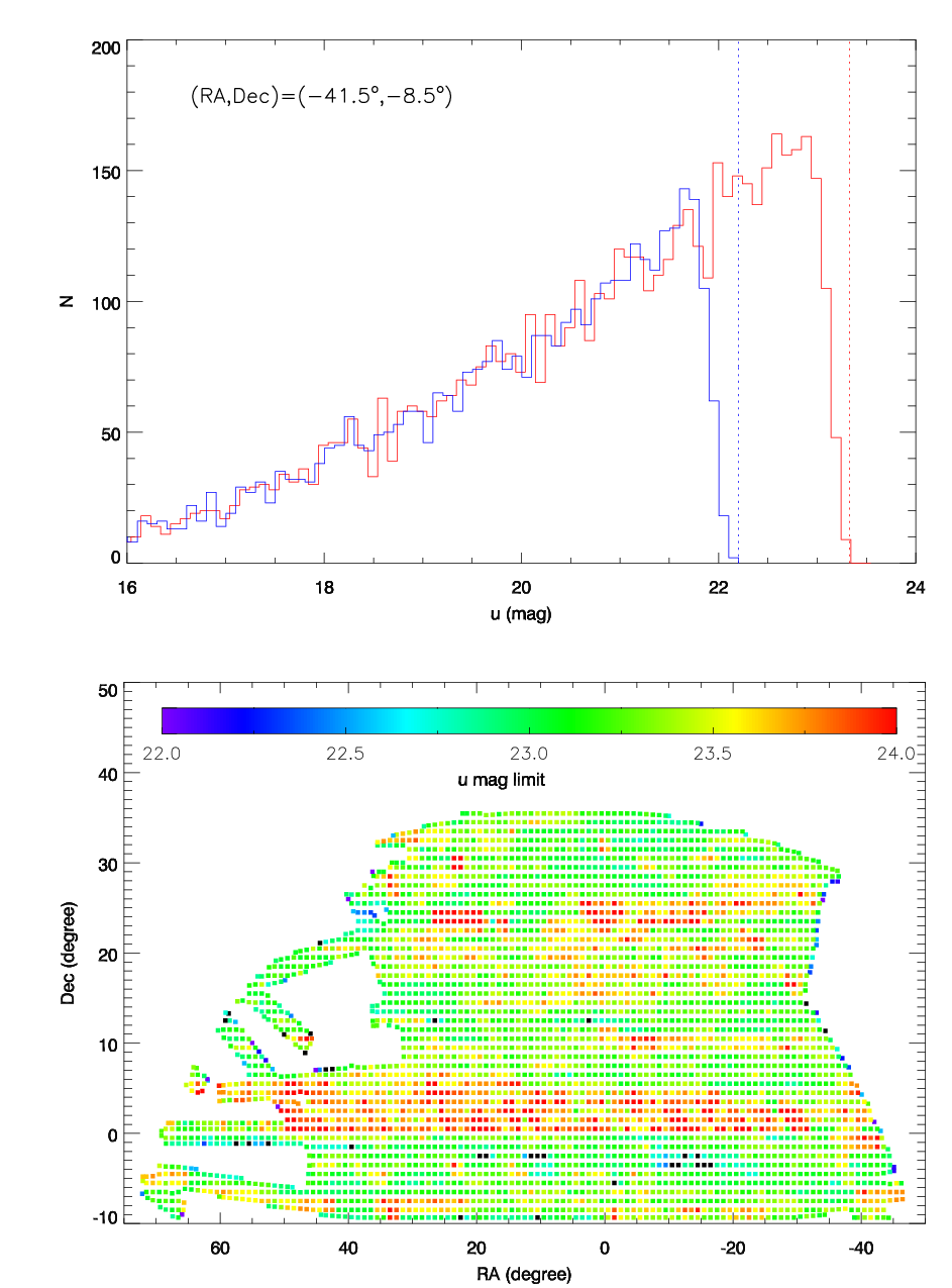
The SCUSS observing strategy yields a significant increase in depth compared to single-epoch SDSS data. We compare these two surveys in Figure 1, where SCUSS co-added PSF magnitudes are compared with SDSS PSF magnitudes. In this figure we divide the whole SCUSS footprint into bins and analyze the magnitude distribution (i.e. luminosity function) of point sources in each bin, where star-galaxy separation is based on the SDSS classification. The luminosity function turns over at faint magnitudes as the survey reaches its detection limit and becomes incomplete. In our case the limiting magnitude is defined as the maximum magnitude of a star with a given error. For both SDSS & SCUSS datasets we consider detections with -band photometric error less than 0.2 mag (5). This procedure is illustrated in the top panel of Figure 1. For this example field (located at ) we find that the SCUSS magnitude limit is around 23.3, which is around 1 mag deeper than SDSS. The bottom panel of this figure shows the distribution of magnitude limit across the SCUSS footprint. In general the SCUSS fields are 1 to 1.5 mag deeper. As our BHB classification requires photometry, we have only analyzed the 3400 sq. deg. of the SCUSS footprint that overlaps with SDSS. As can be seen from this figure, the overlap region is not contiguous due to the incomplete SDSS coverage for . The resulting depth varies somewhat across the footprint, but for most fields the limiting magnitude lies in the range 23 to 24 mag. Completeness for a given field is related to the turn-over in this luminosity function, which is typically 0.5 mag brighter than the limiting magnitude. We have also measured the location of this turn-over for each field and find that only 2 per cent have a value brighter than 21.5 mag. For a BHB star this magnitude corresponds to a distance of around 100 kpc, so we are confident that our BHB samples should be reasonably complete to 100 kpc and are able to probe significantly further than this (albeit at lower completeness).
III. BHB selection
The class of A-type stars, which includes BHBs, can be selected using a color-color box in the space of ()0 vs ()0. In the following work all magnitudes are corrected for extinction (labeled with a subscript ‘0’) using the maps of Schlegel et al. [20] and adopting the reddening conversions from Schlafly & Finkbeiner [21]. For SCUSS objects with and error less than 0.2, the A-type stars are selected following [31, 23],
| (1) |
The color-color criterion is efficient at removing contamination of non-A-type main-sequence stars, white dwarfs and most of the quasars. To further eliminate quasars from the A-type sample we use the following color cut [9, similar to],
| (2) |
This cut removes many spurious points at the left and right edges of the ()0 vs ()0 diagram, making the BHB claw look more distinct. By cross-matching with SDSS spectroscopy we found that many of the points removed by the color cuts in Equation (2) are indeed quasars. In order to check how many potential quasars are left in the resulting sample, we apply the XDQSO22 2 http://www.sdss3.org/svn/repo/xdqso/tags/v0-6/doc/build/html/index.html technique [4, 5], which has been designed to use for the SDSS quasar targeting selection. We found that the number of quasars (with probability greater than 0.8) left in our A-type sample is negligible, with a contamination fraction of less than 2%. Deason et al. [9] also demonstrated the efficacy of their cut, finding that their spectroscopic sample of 19 faint () BHBs candidates contained no quasar contamination when this cut was applied. It is possible that there could be some variable star contamination (e.g. RR Lyraes) in the current sample, although it has been estimated that the contamination should only be around 5% and hence this will have little bearing on our results [8]. Also note that since 22.5, which is equivalent to a depth of 21.5, the SDSS star-galaxy separation should be robust [17, see also the SDSS website33 3 https://www.sdss3.org/dr9/imaging/other_info.php].

To select BHB stars from A-type sample, we need to separate them from Blue Stragglers (BS). BS stars also lie in the A-type regime and so are included within our ()0 vs ()0 selection (Equation 1). To discriminate between BHB/BS stars, the ideal approach is to analyze the stars’ spectra, because the two groups have different surface gravities and spectral line profiles [13, 7, 23, 30, 8]. Using spectra from SDSS, Deason et al. [8] separated BHB and BS stars and pinpointed the loci of the two populations in the ()0 vs ()0 color plane. From their color-color diagram, the two groups have a distinct division along the direction (see Figure 2 of Deason et al. 8). This phenomenon is a result of the different surface gravities of BHB and BS stars; since the -band filter is located blue-ward of the Balmer discontinuity, the color characterizes the strength of the Balmer jump, a quantity which is sensitive to the surface gravity. Deason et al. [8] found that the distributions of BHB/BS stars can be fit using one Gaussian for each population, with the center of each Gaussian varying with . By dividing the color-color plane into several slices in , and modeling the BHB/BS distributions of each slice with a two-Gaussian function, one can easily obtain a boundary line for BHB/BS stars.
We classify BHB/BS stars using the above method. However, we cannot directly apply the boundary line of Deason et al. [8] as the filters of SCUSS and SDSS have slightly different profiles [33, 32] and hence objects will have different colors. In order to get an optimal classification for BHB/BS stars we determine our boundary line using only bright stars with accurate photometry, namely and mag. We divide the data along the direction, with widths of 0.02 mag and 0.05 mag. This gives us 18 useful slices which we then fit using two Gaussians,
| (3) |
The fitting procedure is illustrated in the right panel of Figure 2, where we show bin widths of 0.05 mag. The two separate populations can clearly be discerned, with BHB stars lying to the red (i.e. right) side of the distribution. By comparing this figure to the similar one from Deason et al. [8], it is evident that the SCUSS -filter is much more gravity-sensitive, as the BHB/BS populations exhibit less overlap and, in a number of slices, there are clear minima in the distributions. The division is not perfect, meaning that BHB samples will be incomplete and contaminated by BSs (see Section IV), but it is clear that the SCUSS -filter performs better in this regard compared to the SDSS -filter.
The fits for all 18 slices are shown in the left panel of Figure 2, where the red points denote the centers of the Gaussians ( and ), corresponding to the centers of the BS and BHB populations, respectively. We adopt the median of these two values (i.e. ; green points in Figure 2) as the boundary between the two populations. We have chosen to represent the boundary line because this quantity is magnitude independent. For a given slice the ratio of BHB to BS stars () will vary as a function of magnitude, which means that the overall shape of the distribution will alter; however, even though the shape will change, it can be seen that is independent of magnitude. In order to calculate our expression for the boundary line, we fit the values of using the following polynomial function, as shown by the yellow curve in Figure 2:
| (4) |
where stars on the right side of this curve are taken to be BHB stars.
We now apply this classification to the whole magnitude range (), taking all stars with errors in of less than 0.2 mag. As mentioned above, even though Equation (4) was derived for stars with , we are able to apply it now to the full magnitude range because should be independent of magnitude. BHB distances are calculated using Equation (7) of Deason et al. [8], which presents a relation between absolute-magnitude and color with mag.
IV. BHB stars around Pisces
Given this large and relatively clean sample of BHBs, we now proceed to investigate the Pisces overdensity.
We take BHBs according to the boundary defined in Equation (4), but in order to further reduce contamination we reject all stars within 0.02 mag of the boundary and also those which are more than 0.15 mag away, i.e. we only retain stars with mag. The latter cut does not remove many stars, but the former is important for reducing the number of BS contaminants in the sample. Note that although the error cut is 0.2 mag in each band, our final errors are considerably smaller. For example, the median error on for our entire sample is 0.032 mag. Even at faint magnitudes the errors are reasonable, with BHBs at 100 kpc having median error of 0.1 mag.
Since our photometric precision is good and the SCUSS -filter is more sensitive to gravity than the SDSS filter, the level of BS contamination is low. However, as can be seen from the right panel of Figure 2, where it is clear that the BHB and BS Gaussians overlap, this is not negligible and must be estimated. For the typical distances we wish to investigate (i.e. heliocentric distances of 35 to 90 kpc, corresponding to mag), we find that the fraction of BSs contaminating our sample is between 8% and 18%, depending on . As there are no known structures in the foreground of the Pisces region, these BSs should be uniformly distributed and therefore this level of contamination is unlikely to be problematic. Note also that our sample will not be complete, as a number of BHBs lie to the left of the boundary line. We estimate that our BHB sample is around 80% complete.
Now we have our sample of BHBs, we use a standard K-nearest-neighbor algorithm to locate the density peaks. This technique simply calculates the density at a point by averaging over a volume which includes the K nearest neighbors, where the choice of K depends on the problem at hand (in effect this is a smoothing length). For our work we have chosen a value of K10, although our results are similar if one takes K8 or 12. When calculating the density we have subtracted a smooth background model, using a flattened () double power-law profile fit to the RR Lyrae data of Watkins et al. [29]; the fit parameters are given in Faccioli et al. [11, 2nd row of Table 4]. Since this profile corresponds to RR Lyrae and not BHBs, we have increased the normalization by a factor of 2, which we chose in order to match our observed distribution of BHBs. Given this smooth background model, we can calculate the significance of any volume in our 3D space, calculating the difference between the observed and predicted number of BHBs.
We present our map of the BHB density distribution in the left panel of Figure 3. Since the Pisces overdensity was discovered in the SDSS equatorial Stripe 82 data, we first investigate that region (i.e. ). Indeed there is a strong overdensity located around , which is precisely where it was previously identified. The other features of note in this region are the additional structures at , but these are most-likely the edge of the Hercules-Aquila Cloud [2, 27], which was also detected in Stripe 82 [29, e.g.].
When we compare the distance to our Pisces detection (middle panel of Figure 3; again restricting ourselves to just the Stripe 82 region), we find a weak secondary detection behind the main clump at around 95–100 kpc. This more-distant feature has only 5 members and hence may be a spurious detection, but the significance is noticeable (at around 2) because the model predicts very few stars this far out in the halo. The detection is unlikely to be caused by extra-galactic contamination; XDQSO classifies all 5 members as stars and so the overdensity is unlikely to be caused by background quasar contamination and, since mag for these stars, the SDSS star-galaxy classification should be robust [17]. This detection cannot be a ‘shadow’ of mis-classified BSs from the main structure, since the offset in distance modulus is around 0.6 mag, not the 2 mag that one would expect if these were misclassified BSs. Also, with the exception of one star, all are far from the BS/BHB boundary and so this reinforces our belief that these are not BS contaminants.
If one compares our distance distribution to the RR Lyrae detection from Watkins et al. [29, Figure 16], then one also sees a hint of bimodality and a similar spread in distances (around 40 kpc). It should be noted that the peak of our BHB detection is slightly offset from the RR Lyrae detection, with distances of 75 and 80 kpc, respectively. Since there is more uncertainty in the BHB distance calibration (as opposed to the RR Lyrae distances), it may be that this is out by 0.1 to 0.2 mag. This could be due to deficiencies in our adopted absolute-magnitude relation [8, Equation 7], such as a metallicity bias [12], or differences in the adopted extinction values.
The next step is to expand our search beyond the Stripe 82 region. As can be seen the left panel of Figure 3, the wide coverage of the SCUSS data, combined with the clean separation of BHBs from BSs, allows us to tentatively detect an extension of the overdensity to both lower and higher declinations. These manifest themselves as separate clumps, which seem to be connected to the peak overdensity lying at RA and Dec . The significance of these two regions is 3.5 and 3.0, respectively, for the lower- and higher-declination regions. There are some additional clumps at , but again these are most-likely the edge of the Hercules-Aquila Cloud.
It seems that the Pisces overdensity is extended like a stream, passing from the bottom-left to top-right of the figure. In order to confirm this we now analyze the distances of the BHBs in this feature. We define a path for the stream (denoted and ; see Appendix) and take BHBs within 2 deg. The density map of these is shown in the right panel of Figure 3. Here we can see that the detections are aligned beautifully along a distance gradient, confirming our interpretation of a stream. Again the curious cloud of distant BHBs is noticeable beyond 100 kpc, but is clearly unrelated to the stream. The distance gradient along the stream is around 1.3 kpc per deg,
| (5) |
where is the helio-centric distance of the stream in kpc.
We calculate the significance by taking a volume encompassing our Pisces detection and calculating the number of BHB stars predicted from the smooth model, then compare this to the observed number. The model predicts that there should be 8–9 stars in this volume, while we actually find 27 stars. This implies that our detection is 6.2. The significance varies depending on how one defines the background model, for example the flattening or the normalization, but the variation is small and so we conclude that the significance is around 5–7. The significance of the new detections that extend away from the central region, i.e. at and , is 3.5 and 3.3, respectively.
Although we find that 27 stars belong to our detection, this is only an approximate number. As discussed above, some of these may be BS contaminants, while some bona fide BHBs may lie beyond our BHB/BS boundary line. An additional four objects were rejected by our quasar cut (Equation 2), of which two are likely to be stars according to XDQSO. On the other hand, of the 27 objects that passed our quasar cut, one was classified as a quasar by XDQSO.
There are a couple of notes of caution which should be addressed. Firstly, there appears to be a gap in the stream at deg and kpc. We have checked whether this could be due to bad fields or patchy extinction, but neither are found at this location. However, the density of BHBs is low and so this gap could just be due to statistical fluctuations. The other cautionary point is the clump of material around and . Although this is statistically significant (at around 3), the distance distribution is very broad and there is no obvious clumping at the distance of Pisces.

We have chosen to focus on the region around the Pisces overdensity, even though the SCUSS footprint is much larger. However, if we extend the area to the entire footprint, we do not detect any significant new structures.
V. Giant branch exploration
In an attempt to compliment this analysis, we have also analyzed data obtained from the 3.6m Canada-France-Hawaii Telescope (CFHT) using the 1-square-degree field-of-view MegaPrime/MegaCam camera. We chose 8 min exposures in (seeing of 0.5) and 12 min in (seeing of 0.9), allowing us to reach around 24 mag in both bands. Since we could not contiguously map the full region around Pisces, we limited ourselves to 30 pointings (i.e. 30 sq. deg.) spread over a wide area. The location of these fields are shown in the right panel of Figure 4. Although the data reach to 24 mag, the star-galaxy separation (which is dependent on the seeing and signal-to-noise ratio) becomes problematic below around mag. In order to alleviate this problem we cross-match with SCUSS band and apply the following mask to isolate the stellar locus [28, see, for example]
| (6) |
and also apply to remove quasars.
The resulting Hess diagram for our data is shown in the left panel of Figure 4. The main-sequence turn-off for the stellar halo is clearly visible, but there is no obvious detection of any sequence belonging to the Pisces overdensity. To guide the eye, we have included in this figure a box corresponding to the isochrone for an 8 Gyr population with dex, located at 75 kpc. To give the box a finite size we have shifted it by kpc and by mag in . Due to the limitations of the SCUSS data, completeness begins to drop around mag and we are therefore unable to detect the main-sequence turn-off. If the giant branch is present, it is not immediately obvious although it may be hidden behind the main-sequence of the stellar halo, which is considerably more dense.
We investigate further by calculating the number of stars within the isochrone box shown in Figure 4. In order to account for variations in the background density of stars across our fields, we need to normalize this number. We do this by dividing the number of stars inside the isochrone box by , where is the total number of stars in the same magnitude range (, ) excluding stars inside the isochrone box and those within 0.1 mag in of the box boundary. We calculate this fraction as a function of , the cross-stream angle introduced in the previous section and plot this in the middle panel of Figure 4. At most locations this fraction is relatively constant at around 0.425, but for two bins close to the centre of the stream the value is notably above this (at a significance of 1- to 2-, where errors are assumed to be Poissonian).
Finally we split our data into the individual CFHT fields. We first estimate the background by averaging all bins except the two at and 0∘. We then calculate this fraction for each of our fields and, in the right panel of Figure 4 show with filled boxes the fields for which the fraction is at least 0.5 above the background value. From this figure one can see that there is a tendency for fields with larger fractions to lie within 2 deg. of the proposed stream plane (shown by the dashed lines). However, this is inconclusive, with most fields having excess at only 1- to 2-.
In summary, our search for the Pisces giant branch shows tentative evidence for alignment with the stream plane in the previous section, but the results are inconclusive and velocities would be required to clarify the situation.

VI. Discussion
In this paper we have provided an extended view of the Pisces overdensity, utilizing deep band data from the SCUSS survey. With the SCUSS band data, which goes around 1 to 1.5 mag deeper than single-epoch SDSS, we have used BHB stars as tracers and analyzed the distribution of overdensities for 1000 sq. deg. around the original Pisces detection. We have found that Pisces appears to be part of a stream, with a clear distance gradient (Figure 3). This stream is around 5 deg. wide and we appear to trace it for 25 deg. in length. Given the considerable distance to this stream (60 to 80 kpc) this makes it the largest structure (by volume) in the outer halo after the tidal tails of the Sagittarius dwarf galaxy. We find that there are 27 BHBs associated to our extended detection of the overdensity, although we cannot report this number with any high degree of accuracy due to three effects: firstly, some of these BHBs will not belong to the overdensity and are either smooth halo BHBs or foreground BSs; secondly some BHBs will be lost due to incompleteness, especially those which have smaller (bluer) and are hence indistinguishable from BSs; and thirdly, there may be member stars outside the range we have detected. We can roughly estimate the influence of the first two effects, using the contamination and completeness fractions calculated in Section IV. After accounting for these, we predict that total number of BHBs belonging to our Pisecs detection is around 21 stars. With this rough number in hand, we can speculate as to the progenitor of the stream. Assuming we have detected the entire stream and that the progenitor has fully disrupted, then this number of BHBs suggests that the progenitor was likely somewhere between a smaller classical dwarf spheroidal such as Draco or Sextans [1, 16, e.g.], and a larger ultra-faint dwarf like Canes Venatici I [19, e.g.].
Compared to the other Pisces detections, which are restricted to the Stripe 82 region [24, 14, 29, 25], our detection of a tangential extension is new. Before, the only tentative evidence of an extension was reported by Sharma et al. [26]. Using M-giant tracers and a group finding method, they report that the Pisces overdensity extends from RA, Dec, with a distance of 10351 kpc (see Figure 9 of their paper). Compared to our detection, there is a similarity in the region of RA, Dec, but their detection at RA is totally different from ours; here we find the overdensity extending to negative declinations, but the Sharma et al. detection extends to larger positive declinations. Furthermore, this detection does not overlap with the Stripe 82 detection. A more-recent M-giant map of that region is presented [10]. Although not remarked on by the authors themselves, an inspection of the left panel of their Figure 5 shows an overdensity at the same location as the Pisces detection, seemingly oriented in the same direction as our BHB detection.
The only discrepancy between our results and the existing Stripe 82 detections is the offset in distance, with ours being around 10 % smaller than those estimated from RR Lyrae. We are unable to determine the cause of this offset. Like Watkins et al. [29] we also detect a hint that the Stripe 82 detection may be split into a near and far component, but further work needs to be carried out to confirm this. In particular is it unclear whether this could explain the multiple kinematic groups in the Stripe 82 detection, as claimed by Kollmeier et al. [14] and Sesar et al. [25]. It appears that the distances to both features are similar [25, see, for example, Figure 1 of], but with such small numbers of stars it is hard to make firm conclusions. It is also clear that our detection of the stream is rather ‘lumpy’, which may reflect the lumpiness of the stream itself, or possibly due to the sparseness of the tracer population.
Since we have detected a stream, it is natural to ask whether the core of the progenitor remains intact. There is a dwarf galaxy in the vicinity of the stream, the recently detected Pisces II dwarf (RA=344.6∘, Dec=5.9∘) [3]. If we transform its sky coordinates to our stream coordinates, we find that it has and . However, despite it’s close proximity (in projection) to the stream plane, its distance of 180 kpc precludes it from being the progenitor, at least not if it is part of the same wrap of the stream. Given our detected distance gradient, it is now possible to model the orbit of the stream and embark on a large scale hunt for the progenitor.
Appendix A The coordinate transformation
Here, we provide the equations for converting from Equatorial (, ) to the Pisces Overdensity coordinate system (, BP). The orbital pole of the Pisces overdensity is set to (, ), and its center is set to (, ). Details of the derivation are shown below.
Spherical coordinates can be converted to a right-handed Cartesian coordinate system using,
The orbital pole of the Pisces system (, ) can be rotated into the new Cartesian coordinate system as follows,
where
With , and ,
and
where .
If the center of the Pisces overdensity is set to (, ), then we need to put this in phase with the original coordinate system,
where and is for (, )= (, ).
Our orbital plane uses (, ) = (79∘, 47∘) (, ) = (-10∘, 0∘), which results in the following transformation,
| (A1) |
Note that in this system is oriented along the stream and increases with decreasing , and is oriented across the stream and increases with increasing .
The reverse transformation from the Pisces Overdensity coordinate system () to the Equatorial system () is,
| (A2) |
References
- [1] Aparicio, A., Carrera, R., Martínez-Delgado, D. 2001, AJ, 122, 2524
- [2] Belokurov, V., Evans, N. W., Bell, E. F., et al. 2007, ApJ, 657, L89
- [3] Belokurov, V., Walker, M. G., Evans, N. W., et al. 2010, ApJ, 712, L103
- [4] Bovy, J., Hennawi, J. F., Hogg, D. W., et al. 2011a, ApJ, 729, 141
- [5] Bovy, J., Hogg, D. W., & Roweis, S. T. 2011, AnApS, 5, 1657
- [6] Bramich, D. M., Vidrih, S., Wyrzykowski, L., et al. 2008, MNRAS, 386, 887
- [7] Clewley, L., Warren, S. J., Hewett, P. C., et al. 2002, MNRAS, 337, 87
- [8] Deason, A. J., Belokurov, V., & Evans, N. W. 2011, MNRAS, 416, 2903
- [9] Deason, A. J., Belokurov, V., & Evans, N. W. 2012, MNRAS, 425, 2840
- [10] Deason, A. J., Belokurov, V., Hamren, K. M., et al. 2014, 444, 3975
- [11] Faccioli, L., Smith, M. C., Yuan, H.-B., et al. 2014, ApJ, 788, 105
- [12] Fermani, F., Schönrich, R. 2013, MNRAS, 430,1294
- [13] Kinman, T. D., Suntzeff, N. B., & Kraft, R. P. 1994, AJ, 108, 1722
- [14] Kollmeier, J. A., Gould, A., Shectman, S., et al. 2009, ApJ, 705, L158
- [15] Koposov, S. E.,Belokurov, V., Evans, N. W., et al. 2012, ApJ, 750, 80
- [16] Lee, M. G., et al. 2003, AJ, 126, 2840
- [17] Lupton, R. H., Gunn, J. E., Ivezić, Z., Knapp, G. R., & Kent, S. 2001, in ASP Conf. Ser. 238, Astronomical Data Analysis Software and Systems X, ed. F. R. Harnden, F. A. Primini, Jr., & H. E. Payne (San Francisco, CA: ASP), 269
- [18] Newberg, H. J., Yanny, B., & Willett, B. A. 2009, ApJ, 700, L61
- [19] Okamoto, S., Arimoto, N., Yamada, Y., et al. 2012, ApJ, 744, 96
- [20] Schlegel, D. J., Finkbeiner, D. P., & Davis, M. 1998, ApJ, 500, 525
- [21] Schlafly, E. F., & Finkbeiner, D. P. 2011, ApJ, 737, 103
- [22] Stoughton, C., Lupton, R. H., Bernardi, M., et al. 2002, AJ, 123, 485
- [23] Sirko, E., Goodman, J., Knapp, G. R., et al. 2004, AJ, 127, 899
- [24] Sesar, B., Ivezić, Ž., Lupton, R. H., et al. 2007, AJ, 134, 2236
- [25] Sesar, B., Vivas, A. K., Duffau, S., & Ivezić, Ž. 2010, ApJ, 717, 133
- [26] Sharma, S., Johnston, K. V., Majewski, S. R., et al. 2010, ApJ, 722, 750
- [27] Simion, I. T., Belokurov, V., Irwin, M., Koposov, S. E. 2014, MNRAS, 440, 161
- [28] Strateva, I., Ivezić, Ž., Knapp, G. R., et al. 2001, AJ, 122, 1861
- [29] Watkins, L. L., Evans, N. W., Belokurov, V., et al. 2009, MNRAS, 398, 1757
- [30] Xue, X. X., Rix, H. W., Zhao, G., et al. 2008, ApJ, 684, 1143
- [31] Yanny, B., Newberg, H. J., Kent, S., et al. 2000, ApJ, 540, 825
- [32] Zou H., et al. 2015, AJ, submitted
- [33] Zhou X., et al. 2015, RAA, submitted