A Bayesian framework for functional calibration of expensive computational models through non-isometric matching

Experimenting on computational models to understand physical systems has been a popular practice ever since computers became advanced enough to handle complex mathematical models and intense computational procedures (Fang et al., 2005; Santner et al., 2013). This popularity is mainly because a computational model can obtain outputs of an experiment in a relatively more cost-effective and timely manner compared to conducting actual experiments in a laboratory. However, one challenge in utilizing computational models is their “adjustment.” In fact, computational models usually incorporate features that cannot be observed or measured in physical systems, but must be correctly specified so that the computational model can accurately represent the physical system (Kennedy and O’Hagan, 2001). We refer to these unobservable/unmeasurable features as calibration variables, and to the adjustment of their values as the calibration procedure. We call the input features which are common between the computational models and the physical systems as control variables.

For example, in the fabrication of poly-vinyl alcohol (PVA) treated buckypaper, we are interested in understanding the relationship between the response value, which is the tensile strength, and the control variable, which is the PVA amount (Pourhabib et al., 2015). Here, the calibration variable is the percentage of PVA absorbed, which cannot be measured in the physical system, but is required in the computational model.

Past studies on the calibration problem generally assumed unique values for calibration variables, an approach referred to as global calibration, and used different statistical approaches to estimate these values. For instance, Kennedy and O’Hagan (2001); Craig et al. (2001); Reese et al. (2004); Higdon et al. (2004); Higdon et al. (2008); Williams et al. (2006); Bayarri et al. (2007), and Goldstein and Rougier (2009) devised various Bayesian models, whereas Loeppky et al. (2006) and Pratola et al. (2013) used maximum likelihood estimation, and Joseph and Melkote (2009) and Han et al. (2009) developed mixed models by combining frequentist and Bayesian methodologies. More recently Tuo and Wu (2015); Tuo and Wu (2016) developed models based on $L_{2}$ distance projection to estimate the true values of the global calibration variables.

Presently, few studies employ functional calibration by assuming that the values of the calibration variables depend on the control variables. Pourhabib et al. (2015) showed that, for the buckypaper fabrication problem, an approach that considers a parametric functional relationship between the amount of PVA and the percentage absorbed can outperform the global calibration approach of Kennedy and O’Hagan (2001). Similarly, Xiong et al. (2009) used a simple linear relationship to improve the calibration accuracy in a benchmark thermal challenge problem. Furthermore, non-parametric methods can also be utilized to model functional relationships between the calibration variables and the control variables. Such non-parametric functional relationships have been constructed using Reproducing Kernel Hilbert Spaces (Schölkopf et al., 2001) and Gaussian processes (Rasmussen, 2004) by various authors (Pourhabib et al., 2018; Plumlee et al., 2016; Brown and Atamturktur, 2018).

All the aforementioned studies in functional calibration and most studies in global calibration require computational models that are “cheaply executable.” This assumption is required since computational models need to be evaluated thousands of times either to draw samples from a posterior distribution in Bayesian approaches, or to numerically minimize a loss function in other approaches. If the computational model is “expensive,” one can obtain a small number of observations from the computational model, then fit a surrogate function based on these random samples, and in the final step, replace the computational model in the calibration procedure with this new surrogate model. However, as discussed in Section 6, this poses a challenge because “static” replacement may result in poor retrieval of the calibration variables.

Another challenge is the identifiability issue: it is difficult to solve the calibration problem in higher dimensional spaces without making additional assumptions about the solution space (Pourhabib et al., 2018). Furthermore, good prediction performance for the response values does not necessarily imply that a method has accurately captured the functional relationship between the calibration and control variables (Tuo and Wu, 2015; Plumlee and Joseph, 2018; Ezzat et al., 2018). This is a significant drawback since, in many applications, understanding the functional relationship between the calibration and control variables is as important as predicting the response values of the system under study.

In this paper, we develop a new framework for the functional calibration of expensive computational models. Unlike conventional surrogate modeling, which replaces the computational model with a static, approximated surface, we employ a “dynamic” Gaussian process (GP) over the computational model. Our GP is dynamic in the sense that the hyper-parameters of the GP’s covariance function are trained during the calibration procedure. We simultaneously construct posterior distributions for the hyper-parameters of the GP’s covariance function and the calibration variables associated with each of the physical control vectors. In other words, we allow the GP to tune its hyper-parameters in addition to the calibration variables such that the computational model responses become as close as possible to the physical responses.

To tackle the unidentifiability issue in higher-dimensional spaces, we use informative prior distributions. We take advantage of an alternative geometric interpretation of calibration, namely the non-isometric matching of a curve to a surface. We explain this in the case of a single control variable and a single calibration variable. From a geometric perspective, all possible values for the control variable and the physical response constitute a plane curve in the control-response space (see Figure 1(a)). By contrast, in the computational model, we can specify the values of both the control and the calibration variables. Consequently, all possible values of the control and calibration variables, and the responses of the computational model together form a surface. The plane physical curve we observe in the control-response space is a projection of a space curve in the three-dimensional control-calibration-response space. By nature of projection into a lower-dimensional space, the length of the projected curve is not necessarily the same as the original curve in the three-dimensional space. The projection is therefore non-isometric (Bronstein et al., 2003; Bronstein et al., 2005).

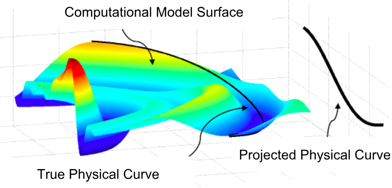
The geometric interpretation is due to the nature of the calibration variable in a physical process: for each value of the control variable there exists a (possibly unknown) value for the calibration variable, and these two features determine a single response. Since we do not observe the actual value of the calibration variable in the physical process, we only see a projected curve in the control-response space. Hence, calibration aims to recover the true physical curve, or in other words, determine a non-isometric match of a curve to a surface.

The remainder of this paper is organized as follows. We explain our Bayesian model for handling expensive computational models in Section 2. Section 3 contains a formal description of the calibration problem and its interpretation as a non-isometric curve to surface matching problem. Our graph-theoretic approach to utilizing this geometric perspective to construct informative prior distributions for our Bayesian model is also presented in Section 3. In Section 4, we generalize the idea of a non-isometric curve to surface matching to higher dimensions and introduce integer programming techniques to tackle the problem. The approach presented in Sections 3 and 4 to construct informative prior distributions for our Bayesian model is used to calculate posterior distributions in Section 5. Our experimental results are reported in Section 6, comparing them with previous approaches. Section 7 concludes the paper and presents paths for future research.

Consider a physical system that operates according to a set of (possibly unknown) physical laws. In this system, there is a functional relationship between a group of features and the response (output). We call those features of the system that can be measured and specified as inputs of the physical system as control variables, and denote the vector of these variables by $\mathbf{x}\in\mathbb{R}^{d^{x}}$. We assume that we obtain data for the physical system by conducting physical experiments: once the control variables are set (either observed or specified) in the physical system, the physical process $\mathcal{F}^{p}$ generates a real-valued response $y^{p}$, that is $y^{p}=\mathcal{F}^{p}(\mathbf{x})$.

Although the response is a function of all features of the physical system, we write $y^{p}$ explicitly as a function of $\mathbf{x}$ as the rest of the features are hard to measure or control, and hence we have no control over them in the physical system. We call such features calibration variables and categorize them into the following two groups: (i) global calibration variables, which have unique values regardless of the values of the control variables, and (ii) functional calibration variables, which are functions of control variables.

We denote the vector of global calibration variables by $\boldsymbol{\psi}\in\mathbb{R}^{d^{\psi}}$ and the vector of functional calibration variables by $\boldsymbol{\theta}\in\mathbb{R}^{d^{\theta}}$. We also denote the function that maps $\mathbf{x}$ to the $k^{\text{th}}$ element of $\boldsymbol{\theta}$, i.e., $\theta_{k}$, by $\mathcal{F}^{\theta}_{k}$ and the vector of all these functions by $\mathcal{F}^{\theta}=[\mathcal{F}^{\theta}_{1},\ldots,\mathcal{F}^{\theta}_{d^{\theta}}]^{\top}$. With a slight abuse of notation, we denote the vector map from $\mathbf{x}$ to $\boldsymbol{\theta}$ using the vector of functions $\mathcal{F}^{\theta}$ as $\boldsymbol{\theta}=\mathcal{F}^{\theta}(\mathbf{x})$.

Suppose we have a computational model constructed according to the laws governing the physical system. Similar to the physical system, the response of our computational model is determined by the interactions between the control and the calibration variables. However, in a computational model we can set the values of all $\mathbf{x}$, $\boldsymbol{\theta}$, and $\boldsymbol{\psi}$ arbitrarily within their respective domains. That is because, unlike physical experiments, there are no constraints on measuring or specifying control or calibration variables in a computational model. If we denote the computational process as $\mathcal{F}^{s}$, then the response of the computational model can be written as,

We refer to obtaining a value for $y^{s}$, given a combination of $\mathbf{x}$, $\boldsymbol{\psi}$, and $\boldsymbol{\theta}$ in the computational model, as a computer experiment.

The goal of calibration is to adjust the variables $\boldsymbol{\psi}\text{ and }\boldsymbol{\theta}$ such that the computational model represents the physical system in the sense that the computational model can predict the physical response at any input location $\mathbf{x}^{*}$.

Mathematically, calibration can be viewed as the estimation of vectors $\mathcal{F}^{\theta}\text{ and }\boldsymbol{\psi}$ such that, for any given $\mathbf{x}^{*}$, the function $\mathcal{F}^{s}:\mathbb{R}^{d^{x}}\times\mathbb{R}^{d^{\psi}}\times\mathbb{R}^{d^{\theta}}\longrightarrow\mathbb{R}$ generates a response close to $y^{p^{*}}$ up to an error $\epsilon^{*}$, i.e.,

where the error $\epsilon^{*}$ captures the measurement error and the discrepancy between the physical and computation model.

To estimate $\boldsymbol{\psi}$ and $\mathcal{F}^{\theta}$ in (2) we initially obtain $m$ responses from $\mathcal{F}^{p}$ at a set of physical system inputs $\{\mathbf{x}^{p}_{1},\ldots,\mathbf{x}^{p}_{m}\}$ to create a dataset $P$ corresponding to that physical system,

We also create the counterpart of $P$ in the computational model, i.e., the computational dataset as

based on a set of computational model inputs $\{(\mathbf{x}^{s}_{1},\boldsymbol{\psi}^{s}_{1},\boldsymbol{\theta}^{s}_{1}),\ldots,(\mathbf{x}^{s}_{n},\boldsymbol{\psi}^{s}_{n},\boldsymbol{\theta}^{s}_{n})\}$. We assume the sets of physical system inputs and the computational model inputs are given. For a discussion of how to select the inputs we refer the reader to the paper by Ezzat et al. (2018).

Let $\boldsymbol{\theta}^{p}_{i}=\mathcal{F}^{\theta}(\mathbf{x}^{p}_{i})$ and $\boldsymbol{\psi}^{p}$ denote the true values of the calibration variables and assume that the errors are independent and have identical normal distribution with zero mean and constant variance. Therefore, we obtain the calibration model as

Note that applying Bayesian statistics to construct posterior distributions for parameters of model (3), i.e., $\boldsymbol{\psi}^{p},\sigma^{2}$ and $\boldsymbol{\theta}^{p}_{i}$, requires a large number of evaluations of $\mathcal{F}^{s}$, which is not practical for expensive computational models. Therefore, we assume $\mathcal{F}^{s}$ is a GP with a constant mean (Rasmussen, 2004), i.e., $\mathcal{F}^{s}\sim\mathcal{GP}(0,\mathcal{K(\cdot,\cdot)})$, where $\mathcal{K(\cdot,\cdot)}$ is a covariance function. We further assume that the overall average of the responses from the computational model has been subtracted from each output, and as such we use a GP with mean zero. Here we use the squared exponential kernel function as the choice of the covariance function,

where $\gamma$ is the magnitude parameter and $\mathbf{L}$ is a diagonal matrix of the length-scale parameters. We denote the vector of the diagonal elements of $\mathbf{L}$ by $\boldsymbol{\ell}$.

Subsequently, we can obtain the likelihood of model (3) by the GP distribution defined on $\mathcal{F}^{s}$ as a multivariate normal distribution,

where $\mathbf{y}^{p}=[y^{p}_{1},\ldots,y^{p}_{m}]^{\top}$ is the vector of physical responses, $\mathbf{X}^{p}=[\mathbf{x}_{1}^{p},\ldots,\mathbf{x}_{m}^{p}]^{\top}$ and $\boldsymbol{\Theta}^{p}=[\boldsymbol{\theta}^{p}_{1},\ldots,\boldsymbol{\theta}^{p}_{m}]^{\top}$ are matrices of size $m\times d^{x}$ and $m\times d^{\theta}$ respectively, and $\boldsymbol{\Sigma}$ is the $m\times m$ covariance matrix whose elements are calculated by covariance function (4) with $[\mathbf{x}^{p^{\top}}_{i},\boldsymbol{\theta}^{p^{\top}}_{i},\boldsymbol{\psi}^{p^{\top}}]^{\top}$ as input vectors with length $(d^{x}+d^{\theta}+d^{\psi})$.

We can estimate the calibration parameters of model (3), the parameters of covariance function (4), and the variance of error, using Bayesian statistics with the posterior distribution,

The Bayesian model (6) would be completed by specifying prior distributions for the parameters $\pi(\boldsymbol{\Theta}^{p})$, $\pi(\boldsymbol{\psi}^{p})$, $\pi(\boldsymbol{\ell})$, $\pi(\gamma)$, and $\pi(\sigma^{2})$. However, our model suffers from unidentifiablity in the absence of informative priors due to the high-dimensionality of the parameter space. Therefore, in Section 5 we present graph-theoretic approaches that help construct informative priors for the calibration parameters $\boldsymbol{\Theta}^{p}$ and $\boldsymbol{\psi}^{p}$.

Note that the replacement of $\mathcal{F}^{s}$ by $\mathcal{GP}(0,\mathcal{K(\cdot,\cdot)})$ does not constitute a surrogate modeling approach, wherein the computational model is replaced by a fixed surrogate surface, which is in turn trained based on a set of limited samples drawn from the computational model prior to any calibration procedure. Our approach is fundamentally different from surrogate modeling, since building and training the GP is a part of the calibration process.

We explain in this section how the calibration problem can be viewed as a non-isometric curve to surface matching problem for the special case where $\mathbf{x}\in\mathbb{R}$, $\boldsymbol{\theta}\in\mathbb{R}$, and $\boldsymbol{\psi}\in\varnothing$, which means both control and calibration variables are one-dimensional and no global calibration variable exists. From a geometric perspective, all the possible values for $\mathbf{x}$ and $\mathcal{F}^{p}(\mathbf{x})$ constitute the curve $(\mathbf{x},\mathcal{F}^{p}(\mathbf{x}))$ in a two-dimensional space. In the computational model, however, we can specify the values of both $\mathbf{x}$ and $\boldsymbol{\theta}$. Consequently, all the possible values of $\mathbf{x}$, $\boldsymbol{\theta}$, and $\mathcal{F}^{s}(\mathbf{x},\boldsymbol{\theta})$ together form a surface $(\mathbf{x},\boldsymbol{\theta},\mathcal{F}^{s}(\mathbf{x},\boldsymbol{\theta}))$ in a three-dimensional space. As we noted in Section 1, the true physical curve lies on the three-dimensional computational model surface, i.e., $(\textbf{x},\mathcal{F}^{\theta}(\mathbf{x}),\mathcal{F}^{p}(\mathbf{x}))$. However, since we do not observe the actual values of the calibration variables in the physical process, we only see a projected curve in $\mathbf{x}-y$ space (see Figure (1(a))). Hence, the calibration problem is to recover the true physical curve, or, in other words, determine a non-isometric match of a curve to a surface.

As mentioned earlier, the non-isometry is due to the fact that the curve $(\textbf{x},\mathcal{F}^{\theta}(\mathbf{x}),\mathcal{F}^{p}(\mathbf{x}))$ on the three-dimensional $\mathbf{x}-\boldsymbol{\theta}-y$ space has a different length than the projected curve $(\mathbf{x},0,\mathcal{F}^{p}(\mathbf{x}))$ on a two-dimensional $\mathbf{x}-y$ space. Therefore, this is, in principle, different from isometric matching problems (Gruen and Akca, 2005; Bronstein et al., 2005; Baltsavias et al., 2008).

In practice we only have the finite physical system dataset $P$ along with a finite computational model dataset $S$, as we do not observe a complete curve or surface. Ideally, the points in $P$ lie on the projected curve that we observe, and the points in $S$ lie on the computational model surface (see Figure 1(b)). Hence, what we observe is incomplete data, and we aim to match non-isometrically an incomplete curve to an incomplete surface, which is equivalent to solving the calibration problem.

This geometric perspective motivates us to view the problem through a combinatorial lens and model the problem using graph-theoretic approaches. Our graph-based solution to the non-isometric curve to surface matching problem provides us with a set of computational model data points, which carry information about the calibration parameters. We call this set of computational data points anchor points. These anchor points will then be used in Section 5 to construct prior distributions for our Bayesian model.

We seek to identify a set of anchor points among the computational data points that are “close” to the points on the true physical curve. In other words, the anchor points are positioned such that the true physical curve passes through the neighborhoods of those points. We want the anchor points to satisfy two desirable properties: (i) the computational model response should be close to the physical response for a given input $\mathbf{x}$; and (ii) the calibration parameter values for two consecutive anchor points should be close to each other. The former drives our method to identify the anchor points that have similar responses to that of the physical system, and the latter aims to encourage the smoothness of the physical curve.

Note that we are only interested in identifying these “optimal” anchor points that provide us with information about the true physical curve to be used in our prior distributions, and not the true physical curve itself. However, one could also directly use the selected anchor points to approximate the true physical curve via interpolation. Given our focus on expensive computational models wherein the number of computational model data points is limited, such an approximation of the true physical curve may not be accurate. In the next section, we formally define and address the problem of finding anchor points with the desired properties using a graph-theoretic approach for the special case when $\mathbf{x}\in\mathbb{R}$, $\boldsymbol{\theta}\in\mathbb{R}$, and $\boldsymbol{\psi}\in\varnothing$.

Section 3 introduced the curve to surface matching interpretation of calibration with $\mathbf{x}\in\mathbb{R}$ and $\boldsymbol{\theta}\in\mathbb{R}$. This special case allowed us to develop a graph-theoretic approach for anchor point selection that admitted a fast $\mathcal{O}(|E|)$ algorithm. The geometric perspective can be generalized to arbitrary dimensions as a hyper-curve to hyper-surface matching problem. However, in the general setting, there is no straightforward extension of the directed acyclic graph model. Recall that the model hinges on the natural ordering of the computational and the physical data points on the real line, which does not exist in higher dimensions. So, in this section we introduce a different calibration graph model and an associated combinatorial optimization problem to find the anchor points in an arbitrary dimension. As with the special case, the anchor points will subsequently be used in Section 5 to construct prior distributions for our Bayesian model.

For the general case, we construct a calibration graph $G=(V,E)$ that is undirected and edge-weighted, where $V=\{1,2,\ldots,n\}$ corresponds to the $n$ computational data points. We partition $V$ into $m$ clusters, $C_{1},\ldots,C_{m}$, in correspondence with the $m$ physical data points and assign vertex $j$ to a cluster $C_{i}$ by the same rule in equation (7). The graph $G$ is a complete $m$-partite graph with partitions $C_{1},\ldots,C_{m}$, i.e., distinct vertices are adjacent if and only if they belong to different partitions. The edge set can be described formally as $E\coloneqq\bigcup_{i=1}^{m-1}\bigcup_{\ell=i+1}^{m}\left\{\{u,v\}\;|\;u\in C_{i},v\in C_{\ell}\right\}.$ Figure 3(a) illustrates this construction.

Finally, before defining the edge weights, we introduce two required concepts. The calibration vector of data point $s_{j}$ is given by $[\boldsymbol{\theta}^{s^{\top}}_{j},\boldsymbol{\psi}^{s^{\top}}_{j}]^{\top}$. We assign the weight $w_{e}$ to the edge $e=\{u,v\}\in E$, where $u\in C_{i}$ and $v\in C_{\ell}$, by

where $\lambda$ is a scaling parameter and $M$ is a sufficiently large number used to penalize the computational data points that are far from each other. Note that the weights assigned in (10) extend the idea behind equation (9). Here, the edge weight between vertices $u\in C_{i}$ and $v\in C_{\ell}$, where $s_{u}$ and $s_{v}$ are neighbors (that is, the Euclidean distance between their control vectors is smaller than a predefined radius $r$), consists of two parts, similar to (9): the first part measures the distance between each vertex’s response and the physical system response associated with the cluster to which it belongs, i.e., $|y_{u}^{s}-y_{i}^{p}|$ and $|y_{v}^{s}-y_{\ell}^{p}|$; the second part measures the distance between the corresponding calibration vectors, i.e., $||[\boldsymbol{\theta}^{s^{\top}}_{u},\boldsymbol{\psi}^{s^{\top}}_{u}]^{\top}-[\boldsymbol{\theta}^{s^{\top}}_{v},\boldsymbol{\psi}^{s^{\top}}_{v}]^{\top}||_{2}$. Let $E_{1}$ denote the set of all edges that join vertex pairs corresponding to control vectors that are at most Euclidean distance $r$ apart. The remainder of the edges, $E_{2}=E\setminus E_{1}$, correspond to edges between computational data points that are not close enough, and we assign relatively large weights to these edges by setting $M$ to a large value. Furthermore, the weight on such edges increases as the distance between the control vectors of the end points increases.

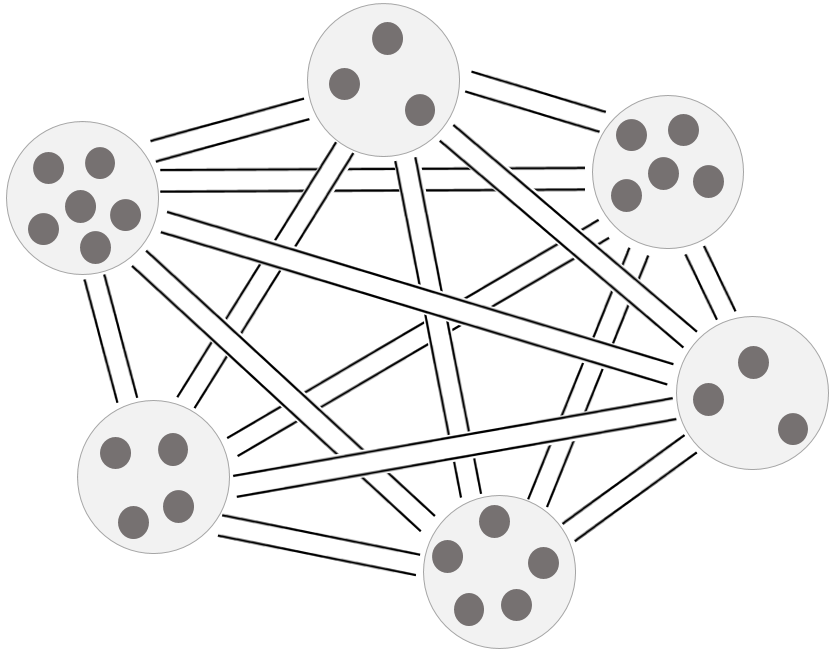
To identify the “optimal” anchor vertices from this calibration graph, we find a minimum weight tree that contains exactly one vertex from each cluster. In the optimization literature, this problem is known as the generalized minimum spanning tree (GMST) problem (Myung et al., 1995). By our construction of the edge weights, a GMST will tend to include edges in $E_{1}$ as they are lighter. However, if no GMST exists that only uses edges in $E_{1}$, it will be forced to include edges in $E_{2}$.

This section describes how the information about the true physical curve carried by the anchor points, found by approaches discussed in Sections 3 and 4, can be used to construct our prior distributions for the calibration parameters. We also expand posterior distribution (6) using the priors specified in this section, and show how we can make predictions at a new control vector $\mathbf{x}^{*}$.

Suppose $\boldsymbol{\theta}^{a}_{i}$ and $\boldsymbol{\psi}^{a}_{i}$ are, respectively, the functional and the global calibration vectors of the anchor point associated with the $i^{th}$ physical data point, i.e., the anchor vertex selected from the $i^{th}$ cluster. Recall that the anchor points are selected by minimizing a weighted combination of two measures: a) the difference between the model responses and physical responses, and b) the distance between the corresponding calibration vectors. As such we can utilize those anchor points to build priors for the calibration parameters in a Bayesian model. To account for the uncertainty associated with the selection of the anchor points, we use variance hyperparameters as explained next. Define the matrix $\boldsymbol{\Theta}^{a}\coloneqq[\boldsymbol{\theta}^{a}_{1},\ldots,\boldsymbol{\theta}^{a}_{m}]^{\top}$ of size $m\times d^{\theta}$ and the mean vector $\boldsymbol{\psi}^{a}\coloneqq\frac{1}{m}\sum_{i=1}^{m}\boldsymbol{\psi}^{a}_{i}$ of length $d^{\psi}$. Note that for the latter we take the average of the global calibration vectors of the anchor points since we assume that the global calibration parameters are constant regardless of the values of the control vectors.

For each component of $\boldsymbol{\psi}^{p}$, the global calibration parameters, we consider a univariate normal distribution centered at the corresponding element in $\boldsymbol{\psi}^{a}$ with an unknown variance as the choice of the prior distribution. Therefore, we construct the prior distribution for $\boldsymbol{\psi}^{p}$ as

where $\boldsymbol{\tau}^{2}=[\tau^{2}_{1},\ldots,\tau^{2}_{d^{\psi}}]^{\top}$ is the vector of variances of the normal distribution.

Applying the same procedure for constructing prior distributions for the functional calibration parameters increases the dimension of the parameter space, since we need to define $md^{\theta}$ variance parameters, which are nuisance parameters and not of interest to our model. Therefore, in order to shrink the parameter space, we use the fact that the $k^{th}$ column of the functional calibration parameters $\boldsymbol{\Theta}^{p}$, i.e. $\boldsymbol{\Theta}^{p}_{k}$, is actually a realization of the functional relationship $\mathcal{F}^{\theta}_{k}$. Therefore, the $k^{th}$ column of $\boldsymbol{\Theta}^{a}$, i.e., $\boldsymbol{\Theta}^{a}_{k}$, is a rough estimator of this realization. On this basis, we use a single variance parameter for all the elements in $\boldsymbol{\Theta}^{p}_{k}$, and construct the prior distribution for $\boldsymbol{\Theta}^{p}_{k}$ as

where $\nu_{k}^{2}$ is the $k^{th}$ element of the vector of variances $\boldsymbol{\nu}^{2}$ with length $d^{\theta}$.

The correctness of the normality assumptions in (11) and (12) is a legitimate concern, because there is no guarantee that the anchor points embrace the true physical curve due to the limited number of observations. However, we only make the normality assumptions in (11) and (12) for constructing the prior distributions, and the Bayesian model will adjust these priors by likelihood (5).

To specify the posterior distribution, we define proper prior distributions for the rest of the parameters. As such, we get:

where,

We refer the reader to Appendix A for the exact prior distributions of parameters in (13), and a discussion of how to sample from the posterior distribution.

In order to make predictions at a new control vector $\mathbf{x}^{*}$, we introduce variables $\boldsymbol{\psi}^{p}(t)$, $\boldsymbol{\ell}(t)$, $\gamma(t)$, $\sigma^{2}(t)$, and $\boldsymbol{\Theta}^{p}(t)$ as $t^{th}$ draws from the posterior distribution (13) after some burn-in period, where $t\in\{1,\ldots,T\}$. The first step in the prediction of response $y^{*}$ is to estimate the associated functional calibration vector of $\mathbf{x}^{*}$, i.e., $\boldsymbol{\theta}^{*}=\mathcal{F}^{\theta}(\mathbf{x}^{*})$. We can estimate $\boldsymbol{\theta}^{*}$ based on each $\boldsymbol{\Theta}^{p}(t)$, where we denote the $t^{\text{th}}$ estimation of $\boldsymbol{\theta}^{*}$ based on $\boldsymbol{\Theta}^{p}(t)$ as $\boldsymbol{\theta}^{*}(t)$. To this end we note that as $\boldsymbol{\Theta}^{p}_{k}(t)$ is a vector of estimates of $\mathcal{F}^{\theta}_{k}$ at the design locations $\{\mathbf{x}^{p}_{1},\ldots,\mathbf{x}^{p}_{m}\}$, we can write $\boldsymbol{\Theta}^{p}_{k}(t)=[\mathcal{F}^{\theta}_{k}(\mathbf{x}_{1}^{p}),\ldots,\mathcal{F}^{\theta}_{k}(\mathbf{x}^{p}_{m})]^{\top}+[\epsilon^{\theta}_{1},\ldots,\epsilon^{\theta}_{m}]^{\top}$, where $[\epsilon^{\theta}_{1},\ldots,\epsilon^{\theta}_{m}]$ is a vector of the corresponding error terms. The error term appears because $\boldsymbol{\Theta}^{p}_{k}(t)$ does not contain exact evaluations of the function $\mathcal{F}^{\theta}_{k}$ but only estimations. The following proposition obtains the mean prediction of $\theta_{k}^{*}(t)$, i.e., the $t^{th}$ estimation of $k^{th}$ element of $\boldsymbol{\theta}^{*}$ base on $\boldsymbol{\Theta}_{k}^{p}(t)$.

To find point and interval predictions for the new response $y^{*}$, we make $T$ predictions based on the $T$ samples we drew from the posterior (13) and the $T$ predictions we made for the vector $\boldsymbol{\theta}^{*}$ using (14). Recall from Section 2 that $\mathcal{F}^{s}\sim\mathcal{GP}(0,\mathcal{K(\cdot,\cdot)})$; therefore, we can use the GP predictive distribution to derive the $t^{th}$ prediction as

where $\mathbf{v}^{*}(t)=[\mathbf{x}^{*^{\top}},\boldsymbol{\theta}^{*^{\top}}(t),\boldsymbol{\psi}^{p^{\top}}(t)]^{\top}$, $\mathbf{V}(t)=[\mathbf{X}^{P},\boldsymbol{\Theta}^{P}(t),\mathbbm{1}_{m\times d_{\psi}}\text{diag}(\boldsymbol{\psi}^{p}(t))]^{\top}$, and the covariance matrices are calculated using the $t^{th}$ sample of the covariance parameters, namely $\boldsymbol{\ell}(t)$ and $\gamma(t)$.

Finally, we derive our prediction using distribution (15) as

In this section, we evaluate the performance of our methodology by testing it on three synthetic problems and two real problems. We use the root mean squared error (RMSE) as the measure of accuracy in prediction of responses and calibration vectors to compare the performance of the competing methodologies;

where $\hat{y_{q}}^{*}$, $\hat{\boldsymbol{\theta}}_{q}^{*}$, and $\hat{\boldsymbol{\psi}}_{q}^{*}$ are the predicted response and calibration parameter values for the $q^{\text{th}}$ test control variable.

Both the MCF and DCSUB formulations find anchor points for each dataset in less than two minutes on all the instances in our testbed, which shows that both formulations are fast in terms of computation time. To choose proper values of $\lambda$, $r$, and $M$ for the GMST model, we use the following empirical approach. First, in order to have the same scale for the inputs and outputs in $S$ and $P$, before constructing the calibration graph we standardize (divide by the range of each element) the control set $\{\mathbf{x}^{p}_{i},\mathbf{x}^{s}_{j}\;|\;i\in\{1,2,\ldots,m\},j\in\{1,2,\ldots,n\}\}$, the calibration set $\{\boldsymbol{\theta}^{s}_{j},\boldsymbol{\psi}^{s}_{j}\;|\;j\in\{1,2,\ldots,n\}\}$, and the response set $\{y^{s}_{j},y^{p}_{i}\;|\;i\in\{1,2,\ldots,m\},j\in\{1,2,\ldots,n\}\}$. We denote the standardized versions of $\mathbf{x}^{p}_{i},\mathbf{x}^{s}_{j},\boldsymbol{\theta}^{s}_{j},\boldsymbol{\psi}^{s}_{j},y^{s}_{j}$, and $y^{p}_{i}$ by $\bar{\mathbf{x}}^{p}_{i},\bar{\mathbf{x}}^{s}_{j},\bar{\boldsymbol{\theta}}^{s}_{j},\bar{\boldsymbol{\psi}}^{s}_{j},\bar{y}^{s}_{j}$, and $\bar{y}^{p}_{i}$. Note that this standardization is only for finding the anchor points, and once the anchor points are chosen, we transform the data back to their original scales for Bayesian inference. After standardization, $\lambda$ has to be less than two, otherwise the closeness of the calibration vectors is weighted as more important than closeness of the responses. We choose $\lambda$ from $\{0.1,0.5,1,1.5\}$ in our experiments. Moreover, for $M$ to be a sufficiently large number, it should be larger than the sum of all the weights on the arcs that can be potentially in $E_{1}$, that is:

Finally, to choose a proper value for $r$, we plot the pairwise Euclidean distances between all $\bar{\mathbf{x}}^{p}$ vectors. Then, we use the fact that each point on this plot represents an existing distance between the centers of two clusters in the calibration graph. Therefore, an upper bound on a group of smallest distances, which are close together and disjoint from other groups of distances, can be used as a proper value for $r$.

We proposed a Bayesian non-isometric matching calibration model for expensive computational models. A limited budget to evaluate computational models led to the use of a GP, which was trained during the calibration procedure. We used Bayesian statistics to simultaneously train the hyper-parameters of the GP’s covariance function and make inferences on the calibration parameters associated with the physical data points. To construct informative prior distributions for our new approach, we used a geometric interpretation of calibration based on non-isometric curve to surface matching. This point of view enabled us to develop graph-theoretic approaches to address the problem of finding a set of anchor points used in constructing informative prior distributions. For the special case of a single control and calibration variable, we introduced a shortest path model on a directed acyclic calibration graph to tackle the problem of finding anchor points, while for the general case, we introduced the generalized minimum spanning tree model. Our numerical experiments conducted on four benchmark calibration problems showed that our approach outperformed the existing calibration models under the assumption of expensive computational models.

The framework developed in this paper could be extended in several ways. We only considered a single computational data point to construct a prior distribution for each calibration parameter; however, information of multiple computational data points could be taken into account. An implementation of this idea, of course, requires developing new combinatorial optimization techniques capable of choosing an appropriate number of computational data points. Another interesting research path would be to consider data uncertainty formally in the calibration graph model instead of using a deterministic calibration graph model, and then using Bayesian inference to deal with the uncertainty in the data. Moreover, one may consider including an independent discrepancy function in equation (3), as noted in Section 2. Finally, the proposed approach would potentially benefit from using cross-validation for the selection of the tuning parameters such as $\lambda$, $r$, and $M$.

Austin Buchanan is supported by the National Science Foundation under Grant No. 1662757. This work was completed utilizing the High Performance Computing Center facilities of Oklahoma State University at Stillwater. The authors also acknowledge Chuck Zhang from Georgia Institute of Technology for providing the authors with the PVA-treated buckypaper fabrication data.

References

- Baltsavias et al. (2008) Baltsavias, E., A. Gruen, H. Eisenbeiss, L. Zhang, and L. Waser (2008). High-quality image matching and automated generation of 3D tree models. International Journal of Remote Sensing 29(5), 1243–1259.
- Bayarri et al. (2007) Bayarri, M. J., J. O. Berger, R. Paulo, J. Sacks, J. A. Cafeo, J. Cavendish, C.-H. Lin, and J. Tu (2007). A framework for validation of computer models. Technometrics 49(2), 138–154.
- Bellman (1958) Bellman, R. (1958). On a routing problem. Quarterly of Applied Mathematics 16(1), 87–90.
- Bertsimas and Weismantel (2005) Bertsimas, D. and R. Weismantel (2005). Optimization Over Integers. Belmont, Massachusetts: Dynamic Ideas.
- Bronstein et al. (2003) Bronstein, A. M., M. M. Bronstein, and R. Kimmel (2003). Expression-invariant 3d face recognition. In International Conference on Audio-and Video-based Biometric Person Authentication, pp. 62–70. Springer.
- Bronstein et al. (2005) Bronstein, A. M., M. M. Bronstein, and R. Kimmel (2005). Three-dimensional face recognition. International Journal of Computer Vision 64(1), 5–30.
- Brown and Atamturktur (2018) Brown, D. A. and S. Atamturktur (2018). Nonparametric functional calibration of computer models. Statistica Sinica 28, 721–742.
- Buchanan et al. (2015) Buchanan, A., J. S. Sung, S. Butenko, and E. L. Pasiliao (2015). An integer programming approach for fault-tolerant connected dominating sets. INFORMS Journal on Computing 27(1), 178–188.
- Craig et al. (2001) Craig, P. S., M. Goldstein, J. C. Rougier, and A. H. Seheult (2001). Bayesian forecasting for complex systems using computer simulators. Journal of the American Statistical Association 96(454), 717–729.
- Ezzat et al. (2018) Ezzat, A. A., A. Pourhabib, and Y. Ding (2018). Sequential design for functional calibration of computer models. Technometrics 60(3), 286–296.
- Fang et al. (2005) Fang, K.-T., R. Li, and A. Sudjianto (2005). Design and modeling for computer experiments. CRC Press.
- Feremans et al. (2002) Feremans, C., M. Labbé, and G. Laporte (2002). A comparative analysis of several formulations for the generalized minimum spanning tree problem. Networks 39(1), 29–34.
- Gelfand et al. (1990) Gelfand, A. E., S. E. Hills, A. Racine-Poon, and A. F. Smith (1990). Illustration of Bayesian inference in normal data models using Gibbs sampling. Journal of the American Statistical Association 85(412), 972–985.
- Gelman et al. (2014) Gelman, A., J. B. Carlin, H. S. Stern, and D. B. Rubin (2014). Bayesian Data Analysis, Volume 2. Chapman & Hall/CRC Boca Raton, FL, USA.
- Goldstein and Rougier (2009) Goldstein, M. and J. Rougier (2009). Reified Bayesian modelling and inference for physical systems. Journal of Statistical Planning and Inference 139(3), 1221–1239.
- Gruen and Akca (2005) Gruen, A. and D. Akca (2005). Least squares 3D surface and curve matching. ISPRS Journal of Photogrammetry and Remote Sensing 59(3), 151–174.
- Han et al. (2009) Han, G., T. J. Santner, and J. J. Rawlinson (2009). Simultaneous determination of tuning and calibration parameters for computer experiments. Technometrics 51(4), 464–474.
- Higdon et al. (2008) Higdon, D., J. Gattiker, B. Williams, and M. Rightley (2008). Computer model calibration using high-dimensional output. Journal of the American Statistical Association 103(482), 570–583.
- Higdon et al. (2004) Higdon, D., M. Kennedy, J. C. Cavendish, J. A. Cafeo, and R. D. Ryne (2004). Combining field data and computer simulations for calibration and prediction. SIAM Journal on Scientific Computing 26(2), 448–466.
- Jeffreys (1946) Jeffreys, H. (1946). An invariant form for the prior probability in estimation problems. Proceedings of the Royal Society of London. Series A, Mathematical and Physical Sciences 186(1007), 453–461.
- Joseph and Melkote (2009) Joseph, V. R. and S. N. Melkote (2009). Statistical adjustments to engineering models. Journal of Quality Technology 41(4), 362.
- Kennedy and O’Hagan (2001) Kennedy, M. C. and A. O’Hagan (2001). Bayesian calibration of computer models. Journal of the Royal Statistical Society: Series B (Statistical Methodology) 63(3), 425–464.
- Lawler (1976) Lawler, E. (1976). Combinatorial Optimization: Networks and Matroids. New York: Holt, Rinehart, and Winston.
- Ljung and Box (1978) Ljung, G. M. and G. E. Box (1978). On a measure of lack of fit in time series models. Biometrika 65(2), 297–303.
- Loeppky et al. (2006) Loeppky, J., D. Bingham, and W. Welch (2006). Computer model calibration or tuning in practice. Technical report, University of British Columbia, Vancouver, BC, CA.
- Lu et al. (2018) Lu, Y., E. Moradi, and B. Balasundaram (2018, November). Correction to: Finding a maximum -club using the -clique formulation and canonical hypercube cuts. Optimization Letters 12(8), 1959–1969.
- Metropolis et al. (1953) Metropolis, N., A. W. Rosenbluth, M. N. Rosenbluth, A. H. Teller, and E. Teller (1953). Equation of state calculations by fast computing machines. The Journal of Chemical Physics 21(6), 1087–1092.
- Moradi and Balasundaram (2018) Moradi, E. and B. Balasundaram (2018, November). Finding a maximum -club using the -clique formulation and canonical hypercube cuts. Optimization Letters 12(8), 1947–1957.
- Myung et al. (1995) Myung, Y.-S., C.-H. Lee, and D.-W. Tcha (1995). On the generalized minimum spanning tree problem. Networks 26(4), 231–241.
- Plumlee and Joseph (2018) Plumlee, M. and V. R. Joseph (2018). Orthogonal Gaussian process models. Statistica Sinica 28(2), 601–619.
- Plumlee et al. (2016) Plumlee, M., V. R. Joseph, and H. Yang (2016). Calibrating functional parameters in the ion channel models of cardiac cells. Journal of the American Statistical Association 111(514), 500–509.
- Pop (2004) Pop, P. C. (2004). New models of the generalized minimum spanning tree problem. Journal of Mathematical Modelling and Algorithms 3(2), 153–166.
- Pop et al. (2006) Pop, P. C., W. Kern, and G. Still (2006). A new relaxation method for the generalized minimum spanning tree problem. European Journal of Operational Research 170(3), 900–908.
- Pourhabib et al. (2015) Pourhabib, A., J. Z. Huang, K. Wang, C. Zhang, B. Wang, and Y. Ding (2015). Modulus prediction of buckypaper based on multi-fidelity analysis involving latent variables. IIE Transactions 47(2), 141–152.
- Pourhabib et al. (2018) Pourhabib, A., R. Tuo, S. He, J. Z. Huang, and Y. Ding (2018). Functional calibration of computer models. Manuscript.
- Pratola et al. (2013) Pratola, M. T., S. R. Sain, D. Bingham, M. Wiltberger, and E. J. Rigler (2013). Fast sequential computer model calibration of large nonstationary spatial-temporal processes. Technometrics 55(2), 232–242.
- Rasmussen (2004) Rasmussen, C. E. (2004). Gaussian Processes for Machine Learning. In Advanced Lectures on Machine Learning, pp. 63–71. Springer.
- Reese et al. (2004) Reese, C. S., A. G. Wilson, M. Hamada, H. F. Martz, and K. J. Ryan (2004). Integrated analysis of computer and physical experiments. Technometrics 46(2), 153–164.
- Santner et al. (2013) Santner, T. J., B. J. Williams, and W. I. Notz (2013). The Design and Analysis of Computer Experiments. Springer Science & Business Media.
- Schölkopf et al. (2001) Schölkopf, B., R. Herbrich, and A. J. Smola (2001). A generalized representer theorem. In International Conference on Computational Learning Theory, pp. 416–426. Springer.
- Shapiro and Wilk (1965) Shapiro, S. S. and M. B. Wilk (1965). An analysis of variance test for normality (complete samples). Biometrika 52(3/4), 591–611.
- Tuo and Wu (2015) Tuo, R. and C. F. J. Wu (2015). Efficient calibration for imperfect computer models. The Annals of Statistics 43(6), 2331–2352.
- Tuo and Wu (2016) Tuo, R. and C. F. J. Wu (2016). A theoretical framework for calibration in computer models: Parametrization, estimation and convergence properties. SIAM/ASA Journal on Uncertainty Quantification 4(1), 767–795.
- Williams et al. (2006) Williams, B., D. Higdon, J. Gattiker, L. Moore, M. McKay, S. Keller-McNulty, et al. (2006). Combining experimental data and computer simulations, with an application to flyer plate experiments. Bayesian Analysis 1(4), 765–792.
- Xiong et al. (2009) Xiong, Y., W. Chen, K.-L. Tsui, and D. W. Apley (2009). A better understanding of model updating strategies in validating engineering models. Computer Methods in Applied Mechanics and Engineering 198(15), 1327–1337.
Appendix A Full and conditional posterior distributions
First, we explain the prior distributions for parameters in (13). We have
For each we use a flat Jeffreys prior (Jeffreys, 1946), which is an inverse gamma distribution with zero value for both the shape and the scale parameter. For each we choose a weak inverse gamma distribution, i.e., an inverse gamma with large variance, with and as its parameters. Note that both of these prior distributions are conjugate for their associated parameters in the posterior distribution. Moreover, as recommended by Gelman et al. (2014), to improve the identifiability of the model we use the prior distributions on the logarithmic scale for parameters of the GP part of the model. Therefore, for and we use a flat log-uniform distribution and for each we use a log-gamma distribution with the parameters .
Using the prior distributions explained above the posterior (13) can be written as