Bayesian Optimal Approximate Message Passing to Recover Structured Sparse Signals
Abstract
We present a novel compressed sensing recovery algorithm – termed BOSSAMP (BOSSAMP) – that jointly exploits the prior distribution and the structured sparsity of a signal that shall be recovered from noisy linear measurements. Structured sparsity is inherent to group sparse and jointly sparse signals. Our algorithm is based on approximate message passing that poses a low complexity recovery algorithm whose Bayesian optimal version allows to specify a prior distribution for each signal component. We utilize this feature in order to establish an iteration-wise extrinsic group update step, in which likelihood ratios of neighboring group elements provide soft information about a specific group element. Doing so, the recovery of structured signals is drastically improved.
We derive the extrinsic group update step for a sparse binary and a sparse Gaussian signal prior, where the nonzero entries are either one or Gaussian distributed, respectively. We also explain how BOSSAMP is applicable to arbitrary sparse signals.
Simulations demonstrate that our approach exhibits superior performance compared to the current state of the art, while it retains a simple iterative implementation with low computational complexity.
Index Terms:
compressed sensing, message passing, group sparse, jointly sparse, sparse binary, Bernoulli-Gaussian, Gaussian mixture, extrinsic information, turbo decodingI Introduction
Solving a linear system of equations for is an omnipresent problem in various fields, as a myriad of problem statements can be written in such form. While the very classical techniques such as least squares or MMSE (MMSE) estimation minimize the error with respect to the -norm, the incorporation of additional knowledge like sparsity and structure of has gained a lot of attention over recent years.
In particular, compressed sensing was introduced in [1, 2, 3] to solve a linear system of equations in case of a sparsely populated , i.e., the vector features only few nonzero entries. A change of paradigm was triggered by recognizing that a sparse can be reconstructed perfectly from an underdetermined system of linear equations. In the context of signal processing, a signal vector can thus be reconstructed from undersampling, where the sampling basis functions are the columns of , and where the samples are stored in . This led to a huge popularity in the search for efficient recovery algorithms that incorporate the sparsity constraint; the classical compressed sensing formulation
where the pseudo norm counts the number of nonzero entries in , leads to a combinatorial search for and is generally NP-hard to solve. The problem was relaxed into an -norm minimization called basis pursuit (denoising) [4] which is also applicable to noisy samples . An alternative formulation that introduces a controllable weight for the sparsity constraint is given by the LASSO (LASSO) [5]. A computationally efficient recovery algorithm that iteratively solves the LASSO is provided by AMP (AMP) that was introduced in [6, 7, 8, 9]. Its foundation is Gaussian loopy belief propagation [10] with simplified message passing that assumes high dimensional signal vectors . Its Bayesian optimal version that exploits the signal prior is described in [7, 8, 9], we will henceforth denote it as BAMP (BAMP). BAMP was further extended in [11] in order to allow for non-linear and non-Gaussian output relations; the samples are transformed by an arbitrary but known function, and the output of the transformation is known to the estimator.
In many problems, features a certain structure in the sparsity, i.e., collections of entries (groups) contain either only zeros or only nonzero entries. Group sparsity typically occurs in (image) classification tasks [12, 13, 14]. To account for this, the LASSO was extended to the group LASSO [15, 16, 17, 18]. Another established scheme is grouped orthogonal matching pursuit [19]. In the realm of AMP, the generalized approach [11] was extended in [20] to incorporate the signal structure.
Aside from group sparsity, structure is also found in jointly sparse signals, i.e., vectors share a common support (the nonzero entries occur at the same indices, ). A prominent instance of this is the multiple measurement vector problem [21, 22]. Typical applications of the jointly sparse case are neuromagnetic imaging [21, 23] and direction-of-arrival estimation [24].
I-A Contributions
In this paper, we present a novel recovery algorithm – termed BOSSAMP – that extends BAMP to incorporate the signal structure, such as group or joint sparsity. The approach also allows for overlapping groups, and it is not restricted to the sparse case. The key feature is the inclusion of a group update step that is inspired by an extrinsic information exchange that is predominantly used in coding [25, 26, 27, 28], where it is also known as the turbo principle. In each iteration of BOSSAMP, the probability that a specific group entry was zero is updated by accumulating the extrinsic information of all other group entries in terms of likelihood ratios. This leads to a superior recovery performance compared to other state of the art approaches such as [19, 20, 18, 17], which we show by simulation. Furthermore, our algorithm converges to a solution in very few iterations, while its implementation stays simple and efficient. Specifically, it only requires two matrix-vector multiplications per iteration, matrix inversions are not required.
I-B Related Work and Novelty
Merging (loopy) belief propagation with turbo equalization to recover structured sparse signals has already been suggested in [29], where the factor graph of the observation structure was extended by a pattern structure. Hidden binary indicators were used to model whether signal entries are active (nonzero) or inactive (zero). Sparsity pattern beliefs are exchanged between the observation structure and the sparsity structure in an iterative manner by leveraging (loopy) belief propagation. This approach was later utilized in compressive imaging [30] to exploit the sparsity and persistence accross scales of 2D wavelet coefficients of natural images. A generalized manifestation of AMP that embeds the ideas of [29] and presents an algorithmic implementation is provided in [20], to which we compare our scheme to.
While [29, 30] approach the topic from the message passing point of view, we focus on an alternative description that utilizes likelihood ratios in terms of -values. We utilize the classic BAMP algorithm and extend the iteration loop by two steps, namely the group update and the subsequent prior update. On the one hand, BAMP assumes independently but non-identically distributed signal entries in to perform scalar MMSE estimation. On the other hand, our two additional steps update the entry-wise prior information for the next BAMP iteration by exploiting the structure in the sparsity. In a ”ping-pong” manner, an MMSE estimate emerges.
We give a detailed and easy-to-follow derivation of the group update step, specifically for the following two prominent cases, where we provide simple closed form expressions: first for the sparse binary case, where -values can be formulated naturally, and then for the sparse Gaussian (also known as Bernoulli-Gaussian) case, where we introduce a latent binary variable that indicates whether an entry was zero or nonzero.
While the resulting BOSSAMP algorithm shares similarities with the HGAMP (HGAMP) algorithm [20] which is applicable to a more general class of problems, our approach sticks to the standard AMP framework [6, 7, 8, 9] which is mainly applicable to samples that are corrupted by Gaussian noise. While being restricted to a smaller class of problems, this leads to a simpler implementation and a higher comprehensibility. Furthermore, simulation results suggest that our approach outperforms HGAMP in terms of recovery performance and phase transitions.
I-C Notation
Boldface letters such as and denote matrices and vectors, respectively. Considering matrix , is its -th row, while is its -th column. The superscript denotes the transposition of a matrix or vector. The vectorization of an matrix is denoted . The identity matrix is denoted . The length all-one vector is denoted , while the all-one matrix is denoted . Similarly, we define the all-zero vector and the all-zero matrix . Calligraphic letters denote sets, their usage as subscript implies that only the vector entries defined by the elements in are selected. The cardinality of a set is denoted by . Random variables and vectors are denoted by sans serif font as and , respectively. While denotes a Gaussian distributed random variable with mean and variance , the shorthand notation
| (1) |
denotes that such a Gaussian distribution is evaluated at the value .
I-D Outline
The remainder of this paper is outlined as follows: section II reviews compressed sensing and draws the link between the probabilistic graphical model of the estimation and the iterative recovery schemes AMP and BAMP, the algorithmic implementation of these is also presented. Finally, two prominent sparse signal priors, namely the sparse binary and the sparse Gaussian prior, are introduced. section III describes the group sparse case and presents the corresponding BOSSAMP algorithm, whose update rules are derived for the sparse binary and the sparse Gaussian signal prior, respectively. section IV does the same for the jointly sparse case. section V discusses the extension of BOSSAMP to the arbitrary signal case. section VI introduces the figures of merit and the comparative schemes for simulation, and then presents and discusses the numerical results. The paper is concluded in section VII.
II Recovery of Sparse Signals
II-A Compressed Sensing
Compressed sensing was introduced in [1, 2, 3] to reconstruct a high-dimensional signal vector from linear measurements
| (2) |
where is the measurement vector, is the fixed sensing matrix and is additive measurement noise. Signal vector is assumed to be -sparse: it has at most out of nonzero entries, where . This enables to recover from eq. 2 although the system of equations is underdetermined. To ensure stable recovery from noisy measurements, the sensing matrix has to satisfy the RIP (RIP) [3]
| (3) |
of order and level for all -sparse vectors , which basically implies that the linear operator preserves the Euclidean distance between every pair of -sparse vectors up to a small constant .
An appropriate sensing matrix can be constructed by picking randomly with i.i.d. (sub-)Gaussian entries. Such matrices were proven in [31] to almost surely satisfy the RIP while the number of required measurements for successful recovery is lower bounded by
| (4) |
where is a small constant and the ceiling operation ensures an integer number of measurements.
II-B Graphical Model
A graphical model poses the probabilistic foundation of compressed sensing recovery algorithms that are based on message passing, such as AMP and BAMP, see [32]. The key ingredient is a factorization of a multivariate distribution – in our case the posterior distribution of given based on eq. 2 – into many factors. This factorization is described and visualized by a factor graph [33, 34], which we will now present.
Let us begin with the underlying probabilistic assumptions. Considering eq. 2, we assume that only sensing matrix is deterministic (fixed), which leaves us to characterize the distributions of measurement vector , signal vector and noise vector .
We assume white Gaussian noise with zero mean and covariance , i.e., . The noise PDF (PDF) calculates as
| (5) |
The joint PDF of signal and measurement can be factored according to Bayes’ rule:
| (6) |
We assume independently distributed signal entries with PDF , the prior, thus, factors as
| (7) |
The likelihood is characterized by the noise PDF:
| (8) |
Estimators of typically rely on the posterior
| (9) |
that entails factors.
The resulting factor graph consists of the variable nodes that encompass the signal of interest , the factor nodes associated to eq. 9, and the edges that correspond to the relations between and which are dictated by the entries of , i.e., . Since typically, all entries of are nonzero, our bipartite graph, as illustrated by fig. 1, is fully connected.

As we intend to recover from knowing , we formulate the MMSE estimator
| (10) |
This task can be approximately11 1 The considered graph typically contains cycles which lead to loopy belief propagation that yields an approximate result. solved utilizing message passing (belief propagation) and the sum-product algorithm [33, 34, 35] on our factor graph. However, a computationally efficient method is only obtained after a series of assumptions and approximations – described in [9] – that yield the AMP algorithm. Note that AMP performs scalar MMSE estimation independently for every component of .
II-C AMP (AMP)
AMP has been introduced in [6, 7, 8, 9] to efficiently solve the LASSO problem [5], also known as basis pursuit denoising [4], that constitutes a non-linear convex optimization problem
| (11) |
The underlying intuition is to find the most accurate solution with the smallest support (motivated by the assumed sparsity of ), where allows for a trade-off between accuracy with respect to the observation error and the sparsity22 2 Sparsity is usually expressed by the -”norm” according to . The -norm relaxation was proven in [1] to very often yield the same result in high dimensions, while introducing a favorable convex optimization problem. of the solution.
An illustrative approach to obtain the LASSO from MMSE estimator eq. 10 is to assume that the signal vector entries are Laplacian distributed, i.e., with
| (12) |
The zero mean Laplace distribution poses a sparsity enforcing prior, i.e., its probability mass is concentrated around zero. Plugging the Laplace signal prior into eq. 9 and calculating the MMSE estimate eq. 10, we obtain the LASSO eq. 11 with .
In AMP, is a design parameter. For the optimal choice of , it was shown in [36] that the fixed point of the AMP solution conicides with the LASSO solution in the asymptotic regime where while .
As discussed in [37, 32], AMP decouples the estimation problem associated to measurement eq. 2 into uncoupled scalar problems in the asymptotic regime:
| (13) |
where the effective noise asymptotically obeys . Note that it is Gaussian33 3 This is an assumption that is satisfied in the asymptotic regime., and . Revisiting the LASSO problem in the scalar case, i.e.,
| (14) |
it is known that the soft thresholding function
| (15) |
admits a (possibly optimal) solution to eq. 14, see [5]. The soft thresholding function acts as a denoiser, i.e., it sets values below a certain threshold to zero. This function is also found in the AMP algorithm – our implementation is stated by Algorithm 1 – where it is applied entry-wise on the decoupled measurements , i.e., on . The iterations are stopped once the change in the estimated signal is below a certain threshold – controlled by – or the maximal number of iterations is reached. For a detailed derivation of AMP, the interested reader is refered to [6, 7, 8, 9].
II-D BAMP (BAMP)
While the standard AMP algorithm implicitly assumes a (sparsity enforcing) Laplacian signal prior, its Bayesian optimal version BAMP allows to specify arbitrary signal priors , individually for each entry of the signal vector — this is a key feature that will be exploited by the proposed algorithms for structured sparsity. As before, we will stick to the main features and refer to [7, 8, 9] for details.
BAMP builds on the same decoupling principle [37, 32] as AMP, which is valid in the asymptotic regime and approximately satisfied in finite dimensions. Let us discuss the decoupled scalar problem eq. 13, , where we know that . The (entry-wise) posterior of the decoupled problem thus reads, using Bayes’ theorem,
| (16) |
where and . Instead of soft thresholding, BAMP utilizes the following functions [7, 8, 9]:
| (17) | ||||
| (18) | ||||
| (19) |
The conditional expectation eq. 17 yields the scalar MMSE estimate of given the decoupled measurement . Our implementation of BAMP is stated by Algorithm 2. Function eq. 17 is applied entry-wise on a vector argument, eq. 18 is typically an intermediate step to compute eq. 19. Note that for a specified signal prior, functions eqs. 17, 18 and 19 admit closed form expressions. We will now specify those for a sparse binary and a sparse Gaussian signal prior, respectively.
- Sparse Binary Signal Prior:
- Sparse Gaussian Signal Prior:
If the number of nonzero entries is known a priori, we choose
| (30) |
In case uf unknown sparsity, one has to assume a certain sparsity and plug in an estimate for .
III Recovery of Group Sparse Signals
In the group sparse case, signal vector is partitioned into groups such that the groups partition (non-overlapping case) the total support set :
| (31) |
where contains the signal vector indices that correspond to group . In case of overlapping groups, the intersection of two different groups may contain elements. The signal vector entries that correspond to a group are either all zero or all nonzero — knowing the groups reflects the a priori knowledge of the signal structure. An exemplary group assignment on a factor graph is depicted in fig. 2. While the groups may vary in their size , the signal vector is assumed to be -sparse, which typically implies that the number of nonzero groups is small.
Considering BAMP in the sparse signal case, the priors eqs. 20 and 24 allow to modify the probability that a signal entry is zero, for each entry of individually. This is the key feature exploited by BOSSAMP (BOSSAMP).

III-A BOSSAMP and Group Sparse Binary Signals
Binary signals allow for a convenient computation of soft information in terms of -values44 4 -values are log likelihood ratios in the context of coding. They are typically used in soft-input channel decoding or in iterative decoding. [25, 26]:
| (32) |
A large positive value indicates a high probability of being a zero, a large negative value a high probability of being a one. If we consider the decoupled measurements eq. 13, the conditional -values read, using eq. 21,
| (33) | ||||
If we compute the conditional -values in each iteration of BAMP, i.e., compute the likelihood of being a zero for each signal entry estimate, we obtain for entry at iteration (cf. line 6 of Algorithm 2, using eq. 33):
| (34) |
The key feature of BOSSAMP is to use the -values eq. 34 of iteration as extrinsic a priori information [26] in the subsequent iteration . To that end, we calculate the -values that accommodate the innovation of the new iteration:
| (35) |
To exploit the group structure, we introduce the binary extrinsic group update
| (36) | ||||
which yields . This can be interpreted as follows: is the static prior knowledge about the -th entry, and is the extrinsic information of the rest of the group that contains the innovation of the current iteration. If the extrinsic information provides a positive -value, entry becomes more likely to be a zero rather than a one.
After the extrinsic group update, the signal prior is updated accordingly for the subsequent iteration. We therefore introduce the prior update
| (37) |
where we used -value definition eq. 32.
By including these two steps in the BAMP algorithm, we obtain the BOSSAMP algorithm for group sparse signals that is outlined in Algorithm 3 — functions eq. 21, eq. 23 and eq. 36 are utilized for sparse binary signals. The zero probabilities are initialized as , according to eq. 30.
III-B BOSSAMP and Group Sparse Gaussian Signals
In the sparse Gaussian case, we are not able to express -values directly as in the binary case. We tackle this problem by introducing a binary latent random variable inspired by the E-step of the EM (EM) algorithm [38, 39, 40]. This allows us to estimate the zero probabilities in each iteration of BOSSAMP. Consider the prior distribution of the decoupled measurements eq. 13 which can be expressed as a Gaussian mixture[39, 40]:
| (38) | ||||
We distinguish between two Gaussian distributions:
- •
Distribution is associated to the zero entries in the original signal . The corresponding estimates solely contain the effective noise (i.e., ). We thus set and .
- •
Distribution is associated to the nonzeo entries where contains the noisy signal entries (). Therefore, and .
The mixing coefficients determine the probability of the individual mixture components: is the probability of a zero entry, and is the probability of a nonzero entry. In order to estimate these probabilities, a latent binary random variable is introduced:
| (39) |
where and is a Gaussian distribution with mean and variance . Defining the PMF (PMF) of as
| (40) |
the marginalization eq. 39 becomes equivalent to eq. 38 — we successfully reformulated (see [39]) the Gaussian mixture to involve a binary latent variable that can be estimated by the E-step of the EM algorithm. The E-step computes the probabilities
| (41) | ||||
which are called responsibilities; is the responsibility of mixture component for explaining observation . They are used to estimate the zero probabilities in each iteration , which is our E-step. The estimate reads
| (42) |
As our latent variable is binary, we can formulate the -values
| (43) | ||||
that indicate how likely signal entry was to be zero (implies ) given the measurement . Similar to eq. 35, we introduce the innovation -values
| (44) | ||||
They are utilized for the Gaussian extrinsic group update
| (45) |
which is similar to eq. 36. The subsequent prior update is the same as in the binary case, see eq. 37.
The same BOSSAMP algorithm body as stated by Algorithm 3 is used — note that the functions eq. 25, eq. 27 and eq. 45 are utilized for sparse Gaussian signals.
IV Recovery of Jointly Sparse Signals
In the jointly sparse case, we consider signal vectors that share a common support
| (46) |
where contains the indices of the nonzero entries in . In the most general case, the compressive measurements are formulated similar to eq. 2 as
| (47) |
where , , and . Let us collect the data blocks in matrices: , and . If all sensing matrices are equal, i.e., , we can rewrite eq. 47 as
| (48) |
The joint sparsity is expressed by the rows of matrix , whose entries are either all zero or all nonzero. These rows can be interpreted as groups, where each group contains elements. The BOSSAMP algorithm that exploits the joint sparsity is thus very similar to the one in the group sparse case. An exemplary factor graph with blocks is depicted in fig. 3.

IV-A BOSSAMP and Jointly Sparse Binary Signals
Compared to the group sparse case, we essentially have to extend the indexing from vectors to matrices. In particular, contains the zero probabilities of iteration , where is the -th entry of block . Similarly, and , and .
The regular BAMP iteration is executed independently for each of the blocks (jointly sparse signals). Once iteration is finished for all blocks, a collective binary extrinsic group update, similar to eq. 36, is executed to exploit the joint support structure among the signals:
| (49) |
Afterwards, the zero probabilities are updated for the subsequent iteration by executing prior update eq. 37, which is now applied entry-wise on a matrix.
The BOSSAMP algorithm for the jointly sparse case is depicted by Algorithm 4.
IV-B BOSSAMP and Jointly Sparse Gaussian Signals
V Recovery of Arbitrary Structured Signals
While the previous sections presented BOSSAMP for the prominent examples of group/jointly sparse binary and group/jointly sparse Gaussian signals, this section will discuss the generalization to arbitrary signals.
V-A Arbitrary Sparse Signals
BOSSAMP is potentially55 5 At this point, we can not guarantee the stability of loopy belief propagation and BOSSAMP for all arbitrary prior distributions. applicable to arbitrarily distributed signals — the crux is the utilization of the latent variable as demonstrated in the Gaussian case, see section III-B. Soft information in terms of -values is computed and exchanged extrinsically among the group (or joint) structure of the signal(s). In the following, we consider the group sparse case; the jointly sparse case just differs in the indexing as discussed in section IV-A.
Consider an arbitrary sparse signal prior (similar to eqs. 20 and 24)
| (51) |
where is the distribution of the nonzero entries in . Remember that random variable is the sum of the two independent random variables and . The prior distribution of the decoupled measurements (cf. eq. 38 for Gaussian case) is, therefore, obtained via convolution
| (52) | ||||
where . Our zero probability estimates (cf. eq. 42 for Gaussian case) now compute as
| (53) |
and the innovation -values are obtained as
| (54) |
The extrinsic group update is performed with these -values:
| (55) |
Afterwards, prior update eq. 37 is executed.
Following this approach using, e.g., the sparse binary prior eq. 20, the resulting -values eq. 54 coincide with eq. 35. Note, however, that not every arbitrary distribution will entail good recovery performance in the group sparse case; the employed loopy belief propagation at the heart of BOSSAMP may become unstable and require extensions such as damping, see [41, 42].
V-B Arbitrarily Structured Signals
Up to now, we considered either group sparse or jointly sparse signals. It is straightforward to extend BOSSAMP to be applicable to jointly sparse signals that, individually, exhibit a group structure. To that end, the group update has to be extended as follows:
| (56) |
As the signals are jointly sparse, all of them exhibit the same individual group structure, i.e., the same groups . Update eq. 56 accounts for the group as well as the joint sparsity.
VI Comparison and Numerical Results
Let us first introduce the figures of merit for comparison. We then highlight the schemes to which we compare BOSSAMP to. The numerical setup is described, and the simulation results are provided, followed by a discussion. Note that for the sake of brevity, we only present results for the group sparse case.
VI-A Figures of Merit
The measurement SNR (SNR) is defined as
| (57) |
the noise variance is set accordingly for each realization of and to realize a certain SNR during simulation.
The NMSE (NMSE) between original signal and its estimate (recovery) is defined as
| (58) |
it gives indication about the overall recovery performance.
The FANMSE (FANMSE) is defined as
| (59) |
where the complementary signal support contains the indices of the zero entries in . The FANMSE is a measure to quantify the strength of the false alarms in .
VI-B Comparative Schemes
We compare our implementations of AMP, BAMP and BOSSAMP (MATLAB code will be made available at [43]) to the following schemes:
- Group LASSO (GLASSO):
-
in order to incorporate the group structure of , the group LASSO [15, 16, 17] replaces the -norm regularization in eq. 11 with the sum of -norms of the groups:
(60) In case of and , it collapses to the standard LASSO eq. 11.
- Hybrid Generalized Approx. Message Passing (HGAMP):
-
GAMP (GAMP) was introduced in [11] to extend the classical Gaussian AMP framework – on which we build in this paper – to a more general setting that allows for arbitrary output channels and is thus not restricted to additive Gaussian noise in eq. 2. An extension to incorporate structured sparsity was introduced in [20] and is termed HGAMP. It was shown to outperform group orthogonal matching pursuit [19] and the group LASSO in terms of NMSE eq. 58. We use the MATLAB implementation of HGAMP that is provided in [45].
VI-C Numerical Setup
For AMP, BAMP and BOSSAMP, the stopping criterion was set to . The maximum number of iterations was set to , for all algorithms.
For AMP Algorithm 1, we chose (NMSE minimizing heuristic for , see [46]).
For GLASSO, the regularization parameter is chosen according to the example provided in [44], and the augmented Lagrangian and over-relaxation parameters were chosen as and , respectively, as suggested in [44].
For HGAMP with sparse Gaussian signal prior, following options were selected (suggested by the toy example in [45]): step=1, removeMean=true, adaptStep=true. In case of sparse binary signal prior, following options were changed in order to mitigate numerical issues: step=0.1, removeMean=false. In function estim of class GrpSparseEstim.m, the minimum and maximum value of the sparse probability rho was set to and , respectively; the same values where chosen for the minimum and maxium value of pr0 — this improved the recovery performance, and mitigated numerical issues in the binary case.
For the ”variable SNR” and ”variable ” curves, the results are averaged over random realizations. In each realization, sensing matrix and signal vector are newly generated: features i.i.d. zero mean Gaussian entries with unit -norm columns, and has dimension with nonzero entries, entailing a zero probability of . The nonzero entries are one in the sparse binary case eq. 20, and i.i.d. Gaussian with zero mean and variance in the sparse Gaussian case eq. 24. We consider non-overlapping equally-sized groups in and compare three different cases:
- •
Group size . With , this implies that we have active groups out of total groups.
- •
Group size ( active groups).
- •
Group size ( active groups).
For the ”empirical phase transition” curves, we consider an undersampling vs. sparsity grid, where the values range from to with stepsize , respectively. At each grid point, realizations are simulated. Let us introduce a success indicator for each realization :
| (61) |
The average success is obtained as . The empirical phase transition curves are finally obtained by plotting the contour of using MATLAB function contour.
VI-D Numerical Results and Discussion
For convenience, table I highlights how the various schemes utilize prior information, i.e., the sparsity, the Bayesian prior (see eq. 20 and eq. 24), and the group structure. In the following, we call BAMP, BOSSAMP and GAMP the Bayesian message passing-based schemes.
| Sparsity | Bayesian prior | Group structure | |
| GLASSO | ✓ | ✗ | ✓ |
| AMP | ✓ | ✗ | ✗ |
| BAMP | ✓ | ✓ | ✗ |
| BOSSAMP | ✓ | ✓ | ✓ |
| HGAMP | ✓ | ✓ | ✓ |


fig. 4 shows the variable SNR results for the sparse binary case, where the number of measurements was fixed to (inspired by eq. 4 with , see [46]). BOSSAMP, HGAMP and GLASSO depend on the group size that is indicated in brackets, while AMP and BAMP do not exploit the group structure. AMP and GLASSO only include a sparsity constraint steered by in eq. 11 and eq. 60, respectively. BAMP, BOSSAMP and HGAMP exploit the full prior knowledge, i.e., they utilize prior eq. 20. Doing so, these schemes exhibit a steep transition to the success state (), provided that the SNR is sufficiently high. It is evident that larger groups strongly improve the results of the schemes that exploit the group structure, i.e., BOSSAMP, HGAMP and GLASSO. The FANMSE draws a similar picture as the NMSE. It is notable that the GLASSO is able to effectively null the false alarms, given reasonably sized groups. Once the SNR is large enough to ensure successful recovery, the number of iterations of the Bayesian message passing-based schemes stays very low. The overall best recovery performance is obtained by our proposed BOSSAMP algorithm, followed by HGAMP and BAMP.
fig. 5 shows the variable results for the sparse binary case at . We observe very steep success transitions for the Bayesian message passing-based schemes. In particular, BOSSAMP with group size 2 yields successful recoveries above 140 measurements, while for group size 8, it only requires slightly more than 20 measurements. In comparison, HGAMP is successful above 200 and 40 measurements, respectively, and BAMP requires around 300 measurements.


fig. 6 shows the variable SNR results for the sparse Gaussian case with . The message passing-based schemes do not exhibit the same steep success transitions as in the sparse binary case in fig. 4, but a gradually decreasing NMSE over increasing SNR. The performance of BOSSAMP and HGAMP is very similar, particularly for large group sizes. The FANMSE shows a steeper decrease over SNR, and it is again notable that GLASSO features a steep decay, at the expense of stagnating NMSE (the algorithm utilizes thresholding that leads to a sparse solution but lowers the energy in the nonzero entries). GLASSO overall requires the least number of iterations, closely followed by BOSSAMP. However, the Bayesian message passing-based schemes strongly outperform AMP and GLASSO in terms of NMSE and FANMSE.
fig. 7 depicts the variable results for the sparse Gaussian case at . The steep success transitions of the Bayesian message passing-based schemes are back, the NMSE is lower bounded due to finite SNR. It is again evident that BOSSAMP features earlier phase transitions (requires fewer measurements) than HGAMP, which is particularly apparent at small group sizes. The number of iterations behave similarly for BOSSAMP, HGAMP and BAMP; a distinctive peak accompanies the phase transition event, after which the iterations decrease. Due to the same message passing foundation, BOSSAMP and HGAMP behave similarly.
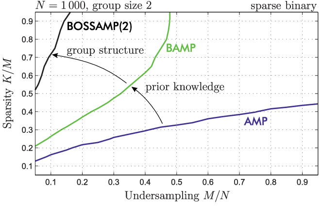

fig. 8 illustrates the empirical phase transition curves for the sparse binary case. The standard AMP algorithm exhibits the worst performance and is strongly surpassed by BAMP that incorporates the Bayesian prior knowledge. Additionally exploiting the group structure leads to a supreme performance which can be seen in the BOSSAMP phase transition curve. Note that the group size in this example was chosen really small as , yet already results in a big improvement.
Finally, fig. 9 illustrates the empirical phase transition curves for the sparse Gaussian case for various group sizes. Clearly, an increase in the group size strongly improves the recovery performance of BOSSAMP and HGAMP and leads to earlier success transitions. While BOSSAMP and HGAMP behave similarly at large values , the strongly undersampled regime causes problems for HGAMP.
VII Conclusion
We introduced BOSSAMP, a novel iterative algorithm to efficiently recover group sparse or jointly sparse signals. The algorithm is based on the AMP framework introduced by Donoho, Maleki and Montanari and exploits the known signal prior distribution. By introducing an extrinsic group update and a prior update step in each iteration, the known signal structure is incorporated into the entry-wise MMSE estimation of the standard BAMP algorithm; considering a specific element of a group, the extrinsic group update step collects soft information from the remaining group elements. -values are accumulated according to the turbo principle and a belief about whether a specific group element was zero or nonzero arises. According to this belief, the subsequent prior update step updates the zero probability of the prior distribution that is utilized for the MMSE estimation in BAMP.
We derived the group update step for the sparse binary respectively the sparse Gaussian case and provided simple closed form expressions. Furthermore, we sketched how BOSSAMP is potentially applicable to arbitrary sparse signals. Simulations have shown that BOSSAMP outperforms current state of the art algorithms, including HGAMP that builds on the same message passing foundation. However, HGAMP is based on GAMP that – in contrast to the standard AMP framework that we utilize in this work – is applicable not only to the additive Gaussian noise case but to a more general class of problems, including nonlinear output relations. While being more general, HGAMP encompasses a more difficult implementation, and simulations suggest that due to a series of (additional) approximations, it sacrifices some performance in comparison to the standard AMP framework [7, 9, 8, 6].
Currently, the signal prior distribution is assumed to be known. For the sparse Gaussian and the more general Gaussian mixture case, the parameters can be estimated using the EM-algorithm, whose application in conjunction with GAMP has been propagated in [47, 48]. Another promising and more general approach was proposed in [49], where Stein’s unbiased risk estimator was incorporated into BAMP.
In conclusion, we have shown that the utilization of the (known) signal structure leads to significant improvements — on the one hand, fewer measurements are required to obtain a certain recovery performance (improved phase transition), while on the other hand, the recovery becomes more robust with respect to noise if the number of measurements is fixed. BOSSAMP is a versatile, easy-to-implement recovery algorithm with great performance.
References
- [1] D. L. Donoho, “Compressed Sensing,” IEEE Transactions on Information Theory, vol. 52, no. 4, pp. 1289–1306, 2006.
- [2] E. J. Candès, J. Romberg, and T. Tao, “Robust uncertainty principles: Exact signal reconstruction from highly incomplete frequency information,” IEEE Transactions on Information Theory, vol. 52, no. 2, pp. 489–509, 2006.
- [3] E. J. Candes, J. K. Romberg, and T. Tao, “Stable signal recovery from incomplete and inaccurate measurements,” Communications on pure and applied mathematics, vol. 59, no. 8, pp. 1207–1223, 2006.
- [4] S. S. Chen, D. L. Donoho, and M. A. Saunders, “Atomic Decomposition by Basis Pursuit,” SIAM journal on scientific computing, vol. 20, no. 1, pp. 33–61, 1998.
- [5] R. Tibshirani, “Regression shrinkage and selection via the lasso,” Journal of the Royal Statistical Society. Series B (Methodological), pp. 267–288, 1996.
- [6] D. L. Donoho, A. Maleki, and A. Montanari, “Message-passing algorithms for compressed sensing,” Proceedings of the National Academy of Sciences, vol. 106, no. 45, pp. 18914–18919, 2009.
- [7] M. A. Maleki, Approximate message passing algorithms for compressed sensing. PhD Thesis, Stanford University, 2010.
- [8] D. L. Donoho, A. Maleki, and A. Montanari, “Message Passing Algorithms for Compressed Sensing: I. Motivation and Construction,” in 2010 IEEE Information Theory Workshop (ITW), pp. 1–5.
- [9] D. L. Donoho, A. Maleki, and A. Montanari, “How to Design Message Passing Algorithms for Compressed Sensing,” preprint, 2011.
- [10] Y. Weiss and W. T. Freeman, “Correctness of belief propagation in Gaussian graphical models of arbitrary topology,” Neural computation, vol. 13, no. 10, pp. 2173–2200, 2001.
- [11] S. Rangan, “Generalized approximate message passing for estimation with random linear mixing,” in IEEE International Symposium on Information Theory Proceedings (ISIT), pp. 2168–2172, IEEE, 2011.
- [12] S. Zhang, J. Huang, Y. Huang, Y. Yu, H. Li, and D. N. Metaxas, “Automatic image annotation using group sparsity,” in IEEE Conference on Computer Vision and Pattern Recognition (CVPR), pp. 3312–3319, IEEE, 2010.
- [13] B. Ng and R. Abugharbieh, “Generalized group sparse classifiers with application in fMRI brain decoding,” in IEEE Conference on Computer Vision and Pattern Recognition (CVPR), pp. 1065–1071, IEEE, 2011.
- [14] J. Gui, D. Tao, Z. Sun, Y. Luo, X. You, and Y. Y. Tang, “Group sparse multiview patch alignment framework with view consistency for image classification,” IEEE Transactions on Image Processing, vol. 23, no. 7, pp. 3126–3137, 2014.
- [15] M. Yuan and Y. Lin, “Model selection and estimation in regression with grouped variables,” Journal of the Royal Statistical Society: Series B (Statistical Methodology), vol. 68, no. 1, pp. 49–67, 2006.
- [16] J. Friedman, T. Hastie, and R. Tibshirani, “A note on the group lasso and a sparse group lasso,” arXiv preprint arXiv:1001.0736, 2010.
- [17] S. Boyd, N. Parikh, E. Chu, B. Peleato, and J. Eckstein, “Distributed optimization and statistical learning via the alternating direction method of multipliers,” Foundations and Trends® in Machine Learning, vol. 3, no. 1, pp. 1–122, 2011.
- [18] W. Deng, W. Yin, and Y. Zhang, “Group sparse optimization by alternating direction method,” in SPIE Optical Engineering+ Applications, pp. 88580R–88580R, International Society for Optics and Photonics, 2013.
- [19] G. Swirszcz, N. Abe, and A. C. Lozano, “Grouped orthogonal matching pursuit for variable selection and prediction,” in Advances in Neural Information Processing Systems, pp. 1150–1158, 2009.
- [20] S. Rangan, A. K. Fletcher, V. K. Goyal, and P. Schniter, “Hybrid generalized approximate message passing with applications to structured sparsity,” in IEEE International Symposium on Information Theory Proceedings (ISIT), pp. 1236–1240, IEEE, 2012.
- [21] S. F. Cotter, B. D. Rao, K. Engan, and K. Kreutz-Delgado, “Sparse solutions to linear inverse problems with multiple measurement vectors,” IEEE Transactions on Signal Processing, vol. 53, no. 7, pp. 2477–2488, 2005.
- [22] J. Ziniel and P. Schniter, “Efficient high-dimensional inference in the multiple measurement vector problem,” IEEE Transactions on Signal Processing, vol. 61, no. 2, pp. 340–354, 2013.
- [23] D. Liang, L. Ying, and F. Liang, “Parallel MRI Acceleration Using M-FOCUSS,” in 3rd International Conference on Bioinformatics and Biomedical Engineering (ICBBE), pp. 1–4, IEEE, 2009.
- [24] G. Tzagkarakis, D. Milioris, and P. Tsak, “Multiple-measurement Bayesian compressed sensing using GSM priors for DOA estimation,” in IEEE International Conference on Acoustics Speech and Signal Processing (ICASSP), pp. 2610–2613, IEEE, 2010.
- [25] J. Hagenauer, “Source-controlled channel decoding,” IEEE Transactions on Communications, vol. 43, no. 9, pp. 2449–2457, 1995.
- [26] J. Hagenauer, E. Offer, and L. Papke, “Iterative decoding of binary block and convolutional codes,” IEEE Transactions on Information Theory, vol. 42, no. 2, pp. 429–445, 1996.
- [27] J. Hagenauer, “The exit chart-introduction to extrinsic information transfer in iterative processing,” in Proc. 12th European Signal Processing Conference (EUSIPCO), pp. 1541–1548, Citeseer, 2004.
- [28] C. Berrou and A. Glavieux, “Near optimum error correcting coding and decoding: Turbo-codes,” Communications, IEEE Transactions on, vol. 44, no. 10, pp. 1261–1271, 1996.
- [29] P. Schniter, “Turbo reconstruction of structured sparse signals,” in 44th Annual Conference on Information Sciences and Systems (CISS), pp. 1–6, IEEE, 2010.
- [30] S. Som and P. Schniter, “Compressive imaging using approximate message passing and a markov-tree prior,” IEEE Transactions on Signal Processing, vol. 60, no. 7, pp. 3439–3448, 2012.
- [31] R. Baraniuk, M. Davenport, R. DeVore, and M. Wakin, “A simple proof of the restricted isometry property for random matrices,” Constructive Approximation, vol. 28, no. 3, pp. 253–263, 2008.
- [32] A. Montanari, “Graphical Models Concepts in Compressed Sensing,” Compressed Sensing: Theory and Applications, pp. 394–438, 2012.
- [33] J. S. Yedidia, “Message-passing algorithms for inference and optimization,” Journal of Statistical Physics, vol. 145, no. 4, pp. 860–890, 2011.
- [34] H.-A. Loeliger, J. Dauwels, J. Hu, S. Korl, L. Ping, and F. R. Kschischang, “The Factor Graph Approach to Model-Based Signal Processing,” Proceedings of the IEEE, vol. 95, no. 6, pp. 1295–1322, 2007.
- [35] F. R. Kschischang, B. J. Frey, and H.-A. Loeliger, “Factor graphs and the sum-product algorithm,” IEEE Transactions on Information Theory, vol. 47, no. 2, pp. 498–519, 2001.
- [36] A. Mousavi, A. Maleki, and R. G. Baraniuk, “Asymptotic Analysis of LASSOs Solution Path with Implications for Approximate Message Passing,” arXiv preprint arXiv:1309.5979, 2013.
- [37] M. Bayati and A. Montanari, “The dynamics of message passing on dense graphs, with applications to compressed sensing,” IEEE Transactions on Information Theory, vol. 57, no. 2, pp. 764–785, 2011.
- [38] A. P. Dempster, N. M. Laird, and D. B. Rubin, “Maximum likelihood from incomplete data via the EM algorithm,” Journal of the royal statistical society. Series B (methodological), pp. 1–38, 1977.
- [39] C. M. Bishop, Pattern recognition and machine learning, vol. 4. springer New York, 2006.
- [40] L. Xu and M. I. Jordan, “On convergence properties of the EM algorithm for Gaussian mixtures,” Neural computation, vol. 8, no. 1, pp. 129–151, 1996.
- [41] T. Heskes, “Stable fixed points of loopy belief propagation are local minima of the bethe free energy,” in Advances in neural information processing systems, pp. 343–350, 2002.
- [42] T. Heskes, “On the uniqueness of loopy belief propagation fixed points,” Neural Computation, vol. 16, no. 11, pp. 2379–2413, 2004.
- [43] M. Mayer and N. Goertz, MATLAB code for AMP, BAMP and BOSSAMP. https://www.nt.tuwien.ac.at/downloads/featured-downloads.
- [44] S. Boyd, N. Parikh, E. Chu, B. Peleato, and J. Eckstein, ADMM group LASSO implementation. https://web.stanford.edu/~boyd/papers/admm/.
- [45] S. Rangan, A. Fletcher, V. Goyal, U. Kamilov, J. Parker, P. Schniter, J. Vila, J. Ziniel, and M. Borgering, GAMP Implementation. http://gampmatlab.sourceforge.net/.
- [46] M. Mayer, N. Goertz, and J. Kaitovic, “RFID Tag Acquisition via Compressed Sensing,” in Proceedings of IEEE RFID Technology and Applications Conference (RFID-TA), pp. 26–31, 2014.
- [47] J. Vila and P. Schniter, “Expectation-maximization Bernoulli-Gaussian approximate message passing,” in Conference Record of the Forty Fifth Asilomar Conference on Signals, Systems and Computers (ASILOMAR), pp. 799–803, IEEE, 2011.
- [48] J. P. Vila and P. Schniter, “Expectation-maximization Gaussian-mixture approximate message passing,” IEEE Transactions on Signal Processing, vol. 61, no. 19, pp. 4658–4672, 2013.
- [49] C. Guo and M. Davies, “Near Optimal Compressed Sensing Without Priors: Parametric SURE Approximate Message Passing,” IEEE Transactions on Signal Processing, vol. 63, pp. 2130–2141, April 2015.