跳到论文正文
W Papers独立论文阅读器 arXiv:1508.01074 论文正文 计算阅读时间 · 0%
引用这篇论文根据当前论文元数据生成,正式投稿前建议核对。


License: arXiv.org perpetual non-exclusive license
arXiv:1508.01074v3 [math.AP] 16 Jun 2016

Small scale equidistribution of eigenfunctions on the torus

Stephen Lester and Zeév Rudnick Address: Department of mathematics, KTH, SE-100 44 Stockholm, Sweden Email address: sjlester@gmail.com Address: Raymond and Beverly Sackler School of Mathematical Sciences, Tel Aviv University, Tel Aviv 69978, Israel Email address: rudnick@post.tau.ac.il
Date: August 24, 2026
Abstract.

We study the small scale distribution of the L2L^{2} mass of eigenfunctions of the Laplacian on the flat torus 𝕋d{\mathbb{T}}^{d}. Given an orthonormal basis of eigenfunctions, we show the existence of a density one subsequence whose L2L^{2} mass equidistributes at small scales. In dimension two our result holds all the way down to the Planck scale. For dimensions d=3,4d=3,4 we can restrict to individual eigenspaces and show small scale equidistribution in that context.

We also study irregularities of quantum equidistribution: We construct eigenfunctions whose L2L^{2} mass does not equidistribute at all scales above the Planck scale. Additionally, in dimension d=4d=4 we show the existence of eigenfunctions for which the proportion of L2L^{2} mass in small balls blows up at certain scales.

1. Introduction

1.1. The semiclassical eigenfunction hypothesis

Let MM be a compact Riemannian manifold (smooth, connected and with no boundary), with associated Laplace-Beltrami operator Δ\Delta, and {ψn}\{\psi_{n}\} an orthonormal basis of L2​(M,dvol)L^{2}(M,\operatorname{dvol}) consisting of eigenfunctions: −Δ​ψn=λn​ψn-\Delta\psi_{n}=\lambda_{n}\psi_{n}, where dvol\operatorname{dvol} is the normalized Riemannian volume form. If the geodesic flow is ergodic, the Quantum Ergodicity Theorem [31, 37, 5] says that for any choice of orthonormal basis (ONB) {ψn}\{\psi_{n}\} consisting of eigenfunctions of the Laplacian, there is a density one subsequence of these eigenfunctions which are uniformly distributed in the unit cotangent bundle S∗​MS^{*}M, where a density one subsequence {ψnℓ}⊂{ψn}\{\psi_{n_{\ell}}\}\subset\{\psi_{n}\} of eigenfunctions is one such that

limΛ→∞#⁡{ψnℓ:λnℓ≤Λ}#{λn≤Λ}=1.\lim_{\Lambda\rightarrow\infty}\frac{\#\{\psi_{n_{\ell}}:\lambda_{n_{\ell}}\leq\Lambda\}}{\#\{\lambda_{n}\leq\Lambda\}}=1.

(For certain chaotic billiards, exceptional eigenfunctions do exist, see [11].) In particular, there is a density-one subsequence of the eigenfunctions so that the probability densities |ψn​(x)|2|\psi_{n}(x)|^{2} converge weakly to the uniform distribution in configuration space MM along this subsequence, i.e. for any (nice) fixed subset Ω⊆M\Omega\subseteq M of positive measure,

1vol⁡(Ω)​∫Ω|ψn​(x)|2​dvol⁡(x)→1.\frac{1}{\operatorname{vol}(\Omega)}\int_{\Omega}|\psi_{n}(x)|^{2}\operatorname{dvol}(x)\to 1\;.

Uniform distribution in configuration space is not only a feature of ergodicity: Marklof and Rudnick [23] show that this is also the case for rational polygons, and for flat tori.

M.V. Berry [1, 2] in his work on the “Semiclassical Eigenfunction Hypothesis” (see also [35]), proposed to go beyond uniform distribution, and study the amplitudes |ψn​(x)|2|\psi_{n}(x)|^{2} when smoothed over regions in MM, whose diameter shrinks as λn→∞\lambda_{n}\to\infty, but at a rate slower than the Planck scale ℏ≈1/λn\hbar\approx 1/\sqrt{\lambda_{n}}, that is to study the local averages

(1.1) 1vol⁡B⁡(xn,rn)​∫B⁡(xn,rn)|ψn​(x)|2​dvol⁡(x)\frac{1}{\operatorname{vol}B(x_{n},r_{n})}\int_{B(x_{n},r_{n})}|\psi_{n}(x)|^{2}\operatorname{dvol}(x)

where B⁡(xn,rn)B(x_{n},r_{n}) is a geodesic ball of radius rnr_{n} centered at xn∈Mx_{n}\in M, so that as λn→∞\lambda_{n}\to\infty, rn→0r_{n}\to 0, but rn​λn→∞r_{n}\sqrt{\lambda_{n}}\to\infty. We will say that small scale equidistribution of the eigenfunctions {ψn}\{\psi_{n}\} holds if (1.1) tends to 11.

There are very few rigorous results on small scale equidistribution in the literature. Luo and Sarnak [21] studied the case of the modular surface, and the orthonormal set of eigenfunctions of the Laplacian which are eigenfunctions of all Hecke operators, showing that for these, small scale equidistribution holds along a density one subsequence for radii r≫λ−αr\gg\lambda^{-\alpha}, for some small α>0\alpha>0. Under the assumption of the Generalized Riemann Hypothesis Young [36] showed that small scale equidistribution holds for all such eigenfunctions for radii r≫λ−1/4+o(1)r\gg\lambda^{-1/4+o(1)}.

The case of compact manifolds with negative sectional curvature was recently investigated independently by Hezari and Rivière [12] and Han [9] who obtained commensurability of the masses along a density one subsequence for logarithmically small radii r=(log⁡λ)−αr=(\log\lambda)^{-\alpha} (0≤α<13​dim⁡MCLOSE(0\leq\alpha<\frac{1}{3\operatorname{dim}M}):

a1≤1vol⁡(B⁡(xn,rn))​∫B⁡(xn,rn)|ψn​(x)|2​dvol⁡(x)≤a2a_{1}\leq\frac{1}{\operatorname{vol}(B(x_{n},r_{n}))}\int_{B(x_{n},r_{n})}|\psi_{n}(x)|^{2}\operatorname{dvol}(x)\leq a_{2}

along the subsequence, where the constants 0<a1<a20<a_{1}<a_{2} are independent of the centers of the balls xnx_{n} and of the subsequence.

1.2. Small scale equidistribution on the flat torus

The case of interest for us is that of the flat dd-dimensional torus 𝕋d=ℝd/2​π​ℤd{\mathbb{T}}^{d}={\mathbb{R}}^{d}/2\pi{\mathbb{Z}}^{d}. The “Semiclassical Eigenfunction Hypothesis” predicts that (1.1) converges to 11 in this setting for radii rn→0r_{n}\rightarrow 0 with rn​λn→∞r_{n}\sqrt{\lambda_{n}}\rightarrow\infty, as λ→∞\lambda\rightarrow\infty. Hezari and Rivière [13] have recently studied small scale equidistribution in 𝕋d{\mathbb{T}}^{d}. They show that for a fixed center x0∈𝕋dx_{0}\in{\mathbb{T}}^{d}, for any ONB of eigenfunctions {ψn}\{\psi_{n}\}, there is a density one subsequence so that for all balls B⁡(x0,rn)B(x_{0},r_{n}) of radius rn>λn−14​(d+1)r_{n}>\lambda_{n}^{-\frac{1}{4(d+1)}} one has that (1.1) tends to 11 along the subsequence.

Note that below the Planck scale r=λ−1/2r=\lambda^{-1/2}, equidistribution fails badly. For example, consider the ONB of eigenfunctions ψμ−​(x)=2​sin⁡(⟨μ,x⟩)\psi^{-}_{\mu}(x)=\sqrt{2}\sin(\langle\mu,x\rangle), ψμ+​(x)=2​cos⁡(⟨μ,x⟩)\psi^{+}_{\mu}(x)=\sqrt{2}\cos(\langle\mu,x\rangle), μ∈ℤd/{±1}\mu\in\mathbb{Z}^{d}/\{\pm 1\}, with eigenvalue λ=|μ|2\lambda=|\mu|^{2}. For r=o(λ−1/2)r=o(\lambda^{-1/2}), and x∈B⁡(0,r)x\in B(0,r) one has ψμ±​(x)∼ψμ±​(0)=1±1\psi^{\pm}_{\mu}(x)\sim\psi^{\pm}_{\mu}(0)=1\pm 1, so that every eigenfunction in this ONB is not equidistributed below the Planck scale.

One of our goals is to prove small scale equidistribution on 𝕋d{\mathbb{T}}^{d}, uniformly for all not too small balls. We succeed for radii rn≫λn−12​(d−1)+o⁡(1)r_{n}\gg\lambda_{n}^{-\frac{1}{2(d-1)}+o(1)}, in particular in dimension d=2d=2, our result extends all the way down to the Planck scale r≫λ−1/2+o(1)r\gg\lambda^{-1/2+o(1)}:

Theorem 1.1.

Let {ψn}\{\psi_{n}\} be an orthonormal basis of eigenfunctions of L2​(𝕋d,dvol)L^{2}({\mathbb{T}}^{d},\operatorname{dvol}), and

ℬn={B⁡(y,r)⊂𝕋d:r>λn−12​(d−1)+o⁡(1)}.\mathcal{B}_{n}=\left\{B(y,r)\subset{\mathbb{T}}^{d}:r>\lambda_{n}^{\frac{-1}{2(d-1)}+o(1)}\right\}.

Then along a density one subsequence,

limn→∞supB⁡(y,r)∈ℬn|1vol⁡(B⁡(y,r))​∫B⁡(y,r)|ψn​(x)|2​dvol⁡(x)−1|=0.\lim_{n\to\infty}\sup_{\begin{subarray}{c}B(y,r)\in\mathcal{B}_{n}\end{subarray}}\left|\frac{1}{\operatorname{vol}(B(y,r))}\int_{B(y,r)}|\psi_{n}(x)|^{2}\,\operatorname{dvol}(x)-1\right|=0\;.

This result gives that the L2L^{2} mass of “almost all” eigenfunctions in the given orthonormal basis is uniformly distributed in every small ball B⁡(y,r)B(y,r). Even though our result does not reach the Planck scale for dimensions d>2d>2, the scale we achieve is actually optimal (up to the λo⁡(1)\lambda^{o(1)} factor). This was pointed out to us by Jean Bourgain (see Remark 1.3 after Theorem 1.2).

1.3. Irregularities in quantum equidistribution

Theorem 1.1 leaves open the existence of exceptional sequences of eigenfunctions. In Theorem 3.1 we show that these do exist, so that one cannot improve the “almost all” statement. We show that there is a sequence of eigenvalues λn→∞\lambda_{n}\to\infty and corresponding L2L^{2}-normalized eigenfunctions ψn\psi_{n} so that for any choice of radii rnr_{n} so that rn→0r_{n}\to 0, but rn​λn→∞r_{n}\sqrt{\lambda_{n}}\to\infty,

limn→∞1vol⁡(B⁡(0,rn))​∫B⁡(0,rn)|ψn​(x)|2​dvol⁡(x)=2.\lim_{n\to\infty}\frac{1}{\operatorname{vol}(B(0,r_{n}))}\int_{B(0,r_{n})}|\psi_{n}(x)|^{2}\operatorname{dvol}(x)=2\;.

For a fixed radius r≈1r\approx 1, see [18] for information on possible “quantum limits”.

In dimension d=4d=4, we can also create “massive irregularities”, where we find an infinite sequence of eigenvalues λn→∞\lambda_{n}\to\infty, so that given any sequence of balls B⁡(xn,rn)B(x_{n},r_{n}) of radius rn≪λ−12​(d−1)−o⁡(1)r_{n}\ll\lambda^{-\frac{1}{2(d-1)}-o(1)}, there are normalized eigenfunctions ψn\psi_{n} whose L2L^{2}-mass on the specific balls B⁡(xn,rn)B(x_{n},r_{n}) blows up:

limn→∞1vol⁡(B⁡(xn,rn))​∫B⁡(xn,rn)|ψn​(x)|2​dvol⁡(x)=∞.\lim_{n\to\infty}\frac{1}{\operatorname{vol}(B(x_{n},r_{n}))}\int_{B(x_{n},r_{n})}|\psi_{n}(x)|^{2}\,\operatorname{dvol}(x)=\infty\;.

A related feature was found on certain negatively curved surfaces by Iwaniec and Sarnak [17], who found eigenfunctions of the Laplacian whose values blow up at special points, see also [24].

On the other hand, in dimension d=2d=2 we rule out the existence of such “massive irregularities” at scales above r>λ−1/4+o(1)r>\lambda^{-1/4+o(1)} and expect that they do not exist at all for r>λ−1/2+o(1)r>\lambda^{-1/2+o(1)}, i.e. just above the Planck scale. We will show that for every eigenfunction ψ⁡(x)\psi(x) in dimension d=2d=2 that for radii r>λ−1/4+o(1)r>\lambda^{-1/4+o(1)}

(1.2) supy∈𝕋21vol⁡(B⁡(y,r))​∫B⁡(y,r)|ψ⁡(x)|2​dvol⁡(x)≪1.\sup_{y\in{\mathbb{T}}^{2}}\frac{1}{\operatorname{vol}(B(y,r))}\int_{B(y,r)}|\psi(x)|^{2}\operatorname{dvol}(x)\ll 1.

The problem of obtaining an upper bound for the proportion of L2L^{2} mass of eigenfunctions in small balls was previously studied by Sogge [32], who showed for any compact dd-dimensional Riemannian manifold (smooth, connected and with no boundary) MM and an L2L^{2}-normalized eigenfunction of the Laplace-Beltrami operator ψ\psi that

supy∈M1vol⁡(B⁡(y,r))​∫B⁡(y,r)|ψ⁡(x)|2​dvol⁡(x)≪r1−d,\sup_{y\in M}\frac{1}{\operatorname{vol}(B(y,r))}\int_{B(y,r)}|\psi(x)|^{2}\operatorname{dvol}(x)\ll r^{1-d},

for r>λ−1/2r>\lambda^{-1/2}.

1.4. Localizing on eigenspaces

In higher dimensions (d≥3d\geq 3), the eigen-spaces have fairly large dimension, and we can also localize on each λ\lambda-eigenspace in dimensions d=3,4d=3,4. That is, prove analogues of Theorem 1.1 when we restrict to an orthonormal basis of an individual eigenspace. For instance, in dimension d=3d=3 for λ≢0,4,7(mod8)\lambda\not\equiv 0,4,7\pmod{8}, the dimension of the λ\lambda-eigenspace, which we denote NλN_{\lambda}, is quite large of size ≈λ12±o⁡(1)\approx\lambda^{\tfrac{1}{2}\pm o(1)}; for d=4d=4 and λ\lambda odd, λ≤Nλ≪λ1+o⁡(1)\lambda\leq N_{\lambda}\ll\lambda^{1+o(1)}. Using results from the arithmetic theory of quadratic forms, we show

Theorem 1.2.

Suppose that d=3d=3 and λ≢0,4,7(mod8)\lambda\not\equiv 0,4,7\pmod{8}, or, d=4d=4 and λ\lambda is odd. Let {ψn}λn=λ\{\psi_{n}\}_{\lambda_{n}=\lambda} be an ONB of eigenfunctions of the λ\lambda-eigenspace and let

ℬλ={B⁡(y,r)⊂𝕋d:r>λ−12​(d−1)+o⁡(1)}.\mathcal{B}_{\lambda}=\left\{B(y,r)\subset{\mathbb{T}}^{d}:r>\lambda^{-\frac{1}{2(d-1)}+o(1)}\right\}.

Then there exists a subset Sλ⊆{ψn}λn=λS_{\lambda}\subseteq\{\psi_{n}\}_{\lambda_{n}=\lambda} of cardinality Nλ​(1+o​(1))N_{\lambda}(1+o(1)), as λ→∞\lambda\rightarrow\infty, which consists of eigenfunctions such that

supB⁡(y,r)∈ℬλ|1vol⁡(B⁡(y,r))​∫B⁡(y,r)|ψn​(x)|2​dvol⁡(x)−1|=o⁡(1),λ→∞,ψn∈Sλ.\sup_{B(y,r)\in\mathcal{B}_{\lambda}}\left|\frac{1}{\operatorname{vol}(B(y,r))}\int_{B(y,r)}|\psi_{n}(x)|^{2}\,\operatorname{dvol}(x)-1\right|=o(1),\quad\lambda\rightarrow\infty,\;\psi_{n}\in S_{\lambda}\;.

Theorem 1.2 reaches the same scale r>λ−12​(d−1)+o⁡(1)r>\lambda^{\frac{-1}{2(d-1)}+o(1)} as Theorem 1.1. Moreover, it gives that the L2L^{2} mass of “almost all” eigenfunctions in the λ\lambda-eigenspace equidistributes inside balls of radii r>λ−12​(d−1)+o⁡(1)r>\lambda^{\frac{-1}{2(d-1)}+o(1)} whereas Theorem 1.1 does not guarantee the existence of even one such eigenfunction. We believe that the analogue of Theorem 1.2 also holds in dimensions d≥5d\geq 5.

Remark 1.3.

Bourgain (private communication) has pointed out that our result is sharp, in that for d≥3d\geq 3, under the conditions on λ\lambda of Theorem 1.2, for radii λ−1/2<r<λ−12​(d−1)−o⁡(1)\lambda^{-1/2}<r<\lambda^{-\frac{1}{2(d-1)}-o(1)} each λ\lambda-eigenspace has an ONB for which a positive proportion of the eigenfunctions fail to equidistribute in B⁡(0,r)B(0,r), in fact for which

1vol⁡(B⁡(0,r))​∫B⁡(0,r)|ψn​(x)|2​dvol⁡(x)∼0,λ→∞.\frac{1}{\operatorname{vol}(B(0,r))}\int_{B(0,r)}|\psi_{n}(x)|^{2}\,\operatorname{dvol}(x)\sim 0,\quad\lambda\to\infty\;.

The construction is detailed in § 4.

1.5. Discrepancy

Given an ONB {ψn}\{\psi_{n}\} consisting of eigenfunctions of the Laplacian, and a∈C∞​(𝕋d)a\in C^{\infty}(\mathbb{T}^{d}), let

V2​(a,Λ):=1#{λn≤Λ}​∑λn≤Λ|∫𝕋da⁡(x)​|ψn​(x)|2​dvol⁡(x)−∫𝕋da⁡(x)​dvol⁡(x)|2.V_{2}(a,\Lambda):=\frac{1}{\#\{\lambda_{n}\leq\Lambda\}}\sum_{\lambda_{n}\leq\Lambda}\left|\int_{\mathbb{T}^{d}}a(x)|\psi_{n}(x)|^{2}\operatorname{dvol}(x)-\int_{\mathbb{T}^{d}}a(x)\operatorname{dvol}(x)\right|^{2}.

Here dvol⁡(x)=d​x/(2​π)d\operatorname{dvol}(x)=dx/(2\pi)^{d} where d​xdx is Lebesgue measure. Marklof and Rudnick [23] showed that V2​(a,Λ)V_{2}(a,\Lambda) decays as Λ→∞\Lambda\to\infty. This was done via arguing as in Schnirelman’s theorem, and using Kronecker’s theorem that generic geodesics are uniformly distributed when projected to configuration space; the point of [23] was that this argument extends to rational polygons. Hezari and Rivière [13] arrive at their results on small scale equidistribution by giving a quantitative rate of decay of V2​(a,Λ)V_{2}(a,\Lambda).

We will derive Theorem 1.1 from an upper bound on the L1L^{1} discrepancy

V1​(a,Λ):=1#{λn≤Λ}​∑λn≤Λ|∫𝕋da⁡(x)​|ψn​(x)|2​dvol⁡(x)−∫𝕋da⁡(x)​dvol⁡(x)|.V_{1}(a,\Lambda):=\frac{1}{\#\{\lambda_{n}\leq\Lambda\}}\sum_{\lambda_{n}\leq\Lambda}\left|\int_{\mathbb{T}^{d}}a(x)|\psi_{n}(x)|^{2}\operatorname{dvol}(x)-\int_{\mathbb{T}^{d}}a(x)\operatorname{dvol}(x)\right|.

For a fixed a trigonometric polynomial, we will show that

(1.3) V1(a,Λ)≪aΛ−1/2.V_{1}(a,\Lambda)\ll_{a}\Lambda^{-1/2}\;.

Note that for chaotic systems, it is expected that the L1L^{1} discrepancy V1​(a,Λ)V_{1}(a,\Lambda) is larger, of size about Λ−1/4\Lambda^{-1/4}, see [6, 7] giving physical arguments for generic chaotic systems, and [22, 19] for rigorous results of this quality for the L2L^{2} discrepancy in arithmetic settings, and [38] for logarithmic upper bounds for the general negatively curved case (see also [29]).

1.6. About the proofs

Our arguments rely upon lattice point estimates in place dynamical properties of the geodesic flow. In particular, the proof of the bound (1.3), given in Section 2.1, combines harmonic analysis and a lattice point argument from the geometry of numbers (see Lemma 2.3). The proof of Theorem 1.2 in Section 5 replaces this lattice point count with a more refined statistic, which counts lattice points on a sphere which lie within a small spherical cap (see Remark 5.4). To estimate this quantity, we require deeper arithmetic information on the number of representations of a positive definite binary quadratic form by sums of squares of linear forms. This is also used in the construction of “massive irregularities” in high dimensions in § 6. Bourgain’s argument, which shows Theorem 1.1 reaches the optimal scale, is detailed in § 4 and also relies upon estimates for the number lattice points within spherical caps. The construction of quantum irregularities in § 3 relies on more direct arguments.

1.7. Notation

Throughout we use the notation, f⁡(x)≪g⁡(x)f(x)\ll g(x), by which we mean f⁡(x)=O⁡(g⁡(x))f(x)=O(g(x)). In addition we write f⁡(x)≫g⁡(x)f(x)\gg g(x) provided there exists a c>0c>0 such that |f⁡(x)|≥c​g​(x)|f(x)|\geq cg(x) for all xx under consideration, and, if f⁡(x)≪g⁡(x)f(x)\ll g(x) and f⁡(x)≫g⁡(x)f(x)\gg g(x) we write f⁡(x)≈g⁡(x)f(x)\approx g(x).

1.8. Acknowledgments

We thank Jean Bourgain, Jon Keating, Stéphane Nonnenmacher, Hamid Hezari, Gabriel Rivière, and Suresh Eswarathasan for their comments on an early version of the paper. The research leading to these results has received funding from the European Research Council under the European Union’s Seventh Framework Programme (FP7/2007-2013) / ERC grant agreement no{}^{\text{o}} 320755.

2. Small scale equidistribution

2.1. L1L^{1} discrepancy on the torus

The goal of this section is to prove the upper bound (1.3) on the L1L^{1} discrepancy.

On the torus 𝕋d\mathbb{T}^{d} each eigenfunction ψn\psi_{n} of −Δ-\Delta with eigenvalue λn\lambda_{n} is of the following form

ψn=∑μ∈ℤd:|μ|2=λncn(μ)eμ\psi_{n}=\sum_{\mu\in\mathbb{Z}^{d}:|\mu|^{2}=\lambda_{n}}c_{n}(\mu)e_{\mu}

where eμ​(x)=ei​⟨μ,x⟩e_{\mu}(x)=e^{{\mathrm{i}}\langle\mu,x\rangle}. Throughout, we assume ψn\psi_{n} is L2L^{2}-normalized so that

∫𝕋d|ψn​(x)|2​dvol⁡(x)=∑|μ|2=λn|cn​(μ)|2=1.\int_{\mathbb{T}^{d}}|\psi_{n}(x)|^{2}\operatorname{dvol}(x)=\sum_{|\mu|^{2}=\lambda_{n}}|c_{n}(\mu)|^{2}=1\;.
Lemma 2.1.

For μ∈ℤd\mu\in\mathbb{Z}^{d} such that |μ|2=λ|\mu|^{2}=\lambda we have

∑λn=λ|cn​(μ)|2=1.\sum_{\lambda_{n}=\lambda}|c_{n}(\mu)|^{2}=1\;.
Proof.

The functions {ψn:λn=λ}\{\psi_{n}:\lambda_{n}=\lambda\} and {eμ:|μ|2=λ}\{e_{\mu}:|\mu|^{2}=\lambda\} are both orthonormal bases of the λ\lambda-eigenspace of −Δ-\Delta, with respect to the inner product

⟨f,g⟩=∫𝕋df⁡(x)​g⁡(x)¯​dvol⁡(x).\langle f,g\rangle=\int_{\mathbb{T}^{d}}f(x)\overline{g(x)}\operatorname{dvol}(x)\;.

Hence in the expansion

ψn=∑|μ|2=λ⟨ψn,eμ⟩​eμ\psi_{n}=\sum_{|\mu|^{2}=\lambda}\langle\psi_{n},e_{\mu}\rangle e_{\mu}

we have

⟨ψn,eμ⟩=cn​(μ)\langle\psi_{n},e_{\mu}\rangle=c_{n}(\mu)

and hence the expansion of eμe_{\mu} is

eμ=∑λn=λ⟨eμ,ψn⟩​ψn=∑λn=λcn​(μ)¯​ψne_{\mu}=\sum_{\lambda_{n}=\lambda}\langle e_{\mu},\psi_{n}\rangle\psi_{n}=\sum_{\lambda_{n}=\lambda}\overline{c_{n}(\mu)}\psi_{n}

and therefore

∑λn=λ|cn​(μ)|2=∑λn=λ|⟨eμ,ψn⟩|2=⟨eμ,eμ⟩=1.\sum_{\lambda_{n}=\lambda}|c_{n}(\mu)|^{2}=\sum_{\lambda_{n}=\lambda}|\langle e_{\mu},\psi_{n}\rangle|^{2}=\langle e_{\mu},e_{\mu}\rangle=1\;.

∎

Lemma 2.2.

If |ζ|≤2​λ|\zeta|\leq 2\sqrt{\lambda} then

∑λn=λ|∫𝕋deζ​(x)​|ψn​(x)|2​dvol⁡(x)|≤#⁡{μ∈ℤd:|μ|2=λ=|μ+ζ|2}.\sum_{\lambda_{n}=\lambda}\left|\int_{\mathbb{T}^{d}}e_{\zeta}(x)|\psi_{n}(x)|^{2}\operatorname{dvol}(x)\right|\leq\#\{\mu\in{\mathbb{Z}}^{d}:|\mu|^{2}=\lambda=|\mu+\zeta|^{2}\}\;.

If |ζ|>2​λ|\zeta|>2\sqrt{\lambda} then each summand is zero.

Proof.

Expand ψn\psi_{n} to get

|∫𝕋deζ​(x)​|ψn​(x)|2​dvol⁡(x)|=|∑|μ|2=λn=|μ+ζ|2cn​(μ)​cn​(μ+ζ)¯|≤∑|μ|2=λn=|μ+ζ|212​|cn​(μ)|2+12​|cn​(μ+ζ)|2.\begin{split}\left|\int_{{\mathbb{T}}^{d}}e_{\zeta}(x)|\psi_{n}(x)|^{2}\operatorname{dvol}(x)\right|&=\left|\sum_{|\mu|^{2}=\lambda_{n}=|\mu+\zeta|^{2}}c_{n}(\mu)\overline{c_{n}(\mu+\zeta)}\right|\\ &\leq\sum_{|\mu|^{2}=\lambda_{n}=|\mu+\zeta|^{2}}\frac{1}{2}|c_{n}(\mu)|^{2}+\frac{1}{2}|c_{n}(\mu+\zeta)|^{2}.\end{split}

Hence,

∑λn=λ|∫𝕋deζ​(x)​|ψn​(x)|2​dvol⁡(x)|≤∑λn=λ∑|μ|2=λn=|μ+ζ|212​|cn​(μ)|2+12​|cn​(μ+ζ)|2=∑|μ|2=λ=|μ+ζ|212​∑λn=λ|cn​(μ)|2+12​∑λn=λ|cn​(μ+ζ)|2=∑|μ|2=λ=|μ+ζ|212+12\begin{split}\sum_{\lambda_{n}=\lambda}\left|\int_{{\mathbb{T}}^{d}}e_{\zeta}(x)|\psi_{n}(x)|^{2}\operatorname{dvol}(x)\right|&\leq\sum_{\lambda_{n}=\lambda}\sum_{|\mu|^{2}=\lambda_{n}=|\mu+\zeta|^{2}}\frac{1}{2}|c_{n}(\mu)|^{2}+\frac{1}{2}|c_{n}(\mu+\zeta)|^{2}\\ &=\sum_{|\mu|^{2}=\lambda=|\mu+\zeta|^{2}}\frac{1}{2}\sum_{\lambda_{n}=\lambda}|c_{n}(\mu)|^{2}+\frac{1}{2}\sum_{\lambda_{n}=\lambda}|c_{n}(\mu+\zeta)|^{2}\\ &=\sum_{|\mu|^{2}=\lambda=|\mu+\zeta|^{2}}\frac{1}{2}+\frac{1}{2}\end{split}

since by Lemma 2.1 both inner sums equal one. Hence,

∑λn=λ|∫𝕋deζ​(x)​|ψn​(x)|2​dvol⁡(x)|≤#⁡{μ∈ℤd:|μ|2=λ=|μ+ζ|2}.\sum_{\lambda_{n}=\lambda}\left|\int_{{\mathbb{T}}^{d}}e_{\zeta}(x)|\psi_{n}(x)|^{2}\operatorname{dvol}(x)\right|\leq\#\{\mu\in{\mathbb{Z}}^{d}:|\mu|^{2}=\lambda=|\mu+\zeta|^{2}\}\;.

Now if |ζ|>2​λ|\zeta|>2\sqrt{\lambda} then there is no (real) solution of |μ|2=λ=|μ+ζ|2|\mu|^{2}=\lambda=|\mu+\zeta|^{2} and hence all terms above vanish. ∎

Lemma 2.3.

For a nonzero integer vector ζ∈ℤd\zeta\in{\mathbb{Z}}^{d} write ζ=m​ζ^\zeta=m\widehat{\zeta}, with m≥1m\geq 1 and ζ^\widehat{\zeta} a primitive integer vector. If 0<|ζ|≤2​X0<|\zeta|\leq 2\sqrt{X} then

#{μ∈ℤd:|μ|2≤X,|μ|2=|μ+ζ|2}≪(X)d−1|ζ^|,\#\{\mu\in{\mathbb{Z}}^{d}:|\mu|^{2}\leq X,|\mu|^{2}=|\mu+\zeta|^{2}\}\ll\frac{(\sqrt{X})^{d-1}}{|\widehat{\zeta}|}\;,

while for |ζ|>2​X|\zeta|>2\sqrt{X}, the set above is empty.

Proof.

Suppose we have a solution μ∈ℤd\mu\in\mathbb{Z}^{d} with |μ+ζ|=|μ|≤X|\mu+\zeta|=|\mu|\leq\sqrt{X} then |ζ|≤|μ+ζ|+|μ|≤2​X|\zeta|\leq|\mu+\zeta|+|\mu|\leq 2\sqrt{X} and hence if |ζ|>2​X|\zeta|>2\sqrt{X} then there are no solutions. So from now on assume |ζ|≤2​X|\zeta|\leq 2\sqrt{X}.

The equality |μ|2=|μ+ζ|2|\mu|^{2}=|\mu+\zeta|^{2} is equivalent to

(2.1) 2​⟨μ,ζ⟩=−|ζ|22\langle\mu,\zeta\rangle=-|\zeta|^{2}

which only has solutions if |ζ|2|\zeta|^{2} is even.

If there are no solutions to (2.1) with |μ|≤X|\mu|\leq\sqrt{X}, then we are done. Otherwise, there exists a solution μ0\mu_{0} and any other such solution satisfies

⟨μ−μ0,ζ⟩=0,|μ−μ0|≤2​X.\langle\mu-\mu_{0},\zeta\rangle=0,\quad|\mu-\mu_{0}|\leq 2\sqrt{X}\;.

We see that the number of solutions |μ|≤X|\mu|\leq\sqrt{X} to (2.1) is bounded by the number of ν∈ℤd\nu\in{\mathbb{Z}}^{d} such that

⟨ν,ζ⟩=0,|ν|≤2​X.\langle\nu,\zeta\rangle=0,\quad|\nu|\leq 2\sqrt{X}\;.

That is, we are counting lattice points in the (d−1)(d-1)-dimensional sub-lattice which is the ortho-complement of ζ\zeta, which lie in a ball. The co-volume (discriminant) of this sub-lattice is |ζ^||\widehat{\zeta}|, where ζ=m​ζ^\zeta=m\widehat{\zeta} with ζ^\widehat{\zeta} primitive, m≥1m\geq 1 integer, and by [28, Section 2] the number of such integer solutions is

cd​(2​X)d−1|ζ^|+O⁡((X)d−2)≪X(d−1)/2|ζ^|,c_{d}\frac{(2\sqrt{X})^{d-1}}{|\widehat{\zeta}|}+O((\sqrt{X})^{d-2})\ll\frac{X^{(d-1)/2}}{|\widehat{\zeta}|},

since |ζ^|≤|ζ|≪X|\widehat{\zeta}|\leq|\zeta|\ll\sqrt{X}. Here cd=πd/2Γ⁡(d2+1)c_{d}=\frac{\pi^{d/2}}{\Gamma(\frac{d}{2}+1)} is the volume of the dd-dimensional unit ball in ℝd\mathbb{R}^{d}. ∎

Proposition 2.4.

If |ζ|≤2​Λ|\zeta|\leq 2\sqrt{\Lambda} then

V1​(eζ,Λ)≪Λ−1/2|ζ^|.V_{1}(e_{\zeta},\Lambda)\ll\frac{\Lambda^{-1/2}}{|\widehat{\zeta}|}\;.

If |ζ|>2​Λ|\zeta|>2\sqrt{\Lambda} then V1​(eζ,Λ)=0V_{1}(e_{\zeta},\Lambda)=0.

Proof.

By Lemma 2.2,

V1​(eζ,Λ)=1#{λn≤Λ}​∑λ≤Λ∑λn=λ|∫𝕋deζ​(x)​|ψn​(x)|2​dvol⁡(x)|≤1#{λn≤Λ}​∑λ≤Λ#⁡{μ∈ℤd:|μ|2=λ=|μ+ζ|2}=1#{λn≤Λ}​#​{|μ|≤Λ:|μ|2=|μ+ζ|2}.\begin{split}V_{1}(e_{\zeta},\Lambda)&=\frac{1}{\#\{\lambda_{n}\leq\Lambda\}}\sum_{\lambda\leq\Lambda}\sum_{\lambda_{n}=\lambda}\left|\int_{\mathbb{T}^{d}}e_{\zeta}(x)|\psi_{n}(x)|^{2}\operatorname{dvol}(x)\right|\\ &\leq\frac{1}{\#\{\lambda_{n}\leq\Lambda\}}\sum_{\lambda\leq\Lambda}\#\{\mu\in{\mathbb{Z}}^{d}:|\mu|^{2}=\lambda=|\mu+\zeta|^{2}\}\\ &=\frac{1}{\#\{\lambda_{n}\leq\Lambda\}}\#\{|\mu|\leq\sqrt{\Lambda}:|\mu|^{2}=|\mu+\zeta|^{2}\}\;.\end{split}

The denominator is #{λn≤Λ}≈Λd/2\#\{\lambda_{n}\leq\Lambda\}\approx\Lambda^{d/2} (Weyl’s law, which follows from an elementary argument since #{λn≤Λ}=#{μ∈ℤd:|μ|2≤Λ}\#\{\lambda_{n}\leq\Lambda\}=\#\{\mu\in\mathbb{Z}^{d}:|\mu|^{2}\leq\Lambda\}), while by Lemma 2.3, the numerator is ≪(Λ)d−1/|ζ^|\ll(\sqrt{\Lambda})^{d-1}/|\widehat{\zeta}|, which gives the claim. ∎

Note that the upper bound (1.3) on the L1L^{1} discrepancy V1​(a,Λ)V_{1}(a,\Lambda) for a general trigonometric polynomial follows from Proposition 2.4.

2.2. Proof of Theorem 1.1

We will need majorants and minorants for the indicator function of a ball. We now cite Lemma 4 of Harman [10] (see also the work of Holt [14] and Holt and Vaaler [15]), which constructs an appropriate version of Beurling-Selberg polynomials:

Lemma 2.5.

Let B⁡(0,r)⊂𝕋dB(0,r)\subset\mathbb{T}^{d} be the ball of radius rr around the origin. Let T,r>0T,r>0 with T​r≥1Tr\geq 1. There exist trigonometric polynomials a±a^{\pm} such that:

  • i)

    a−​(x)≤𝟏B⁡(0,r)​(x)≤a+​(x)a^{-}(x)\leq\mathbf{1}_{B(0,r)}(x)\leq a^{+}(x);

  • ii)

    a^±​(ζ)=0\widehat{a}^{\pm}(\zeta)=0 if |ζ|≥T|\zeta|\geq T;

  • iii)

    a^±​(0)=vol⁡(Bd​(0,r))+Od​(rd−1/T)\widehat{a}^{\pm}(0)=\operatorname{vol}(B_{d}(0,r))+O_{d}(r^{d-1}/T);

  • iv)

    |a^(ζ)|≪drd|\widehat{a}(\zeta)|\ll_{d}r^{d}.

Proof of Theorem 1.1.

Let

ℬn={B⁡(y,r)⊂𝕋d:r>λn−θ1}\mathcal{B}_{n}=\left\{B(y,r)\subset\mathbb{T}^{d}:r>\lambda_{n}^{-\theta_{1}}\right\}

with θ1\theta_{1} to be determined later. Also, for r>λn−θ1r>\lambda_{n}^{-\theta_{1}} let an±a_{n}^{\pm} be the Beurling-Selberg polynomials from Lemma 2.5, which majorize and minorize the indicator function of the ball B⁡(0,r)B(0,r) and also satisfy a^n±​(ζ)=0\widehat{a}_{n}^{\pm}(\zeta)=0 for |ζ|≥Tn=λnθ2|\zeta|\geq T_{n}=\lambda_{n}^{\theta_{2}}, with θ2>θ1\theta_{2}>\theta_{1}. The trigonometric polynomials

bn,y±​(x):=an±​(x−y)b_{n,y}^{\pm}(x):=a_{n}^{\pm}(x-y)

majorize and minorize the translated ball B⁡(y,r)=y+B⁡(0,r)B(y,r)=y+B(0,r), and their Fourier coefficients are given by b^n,y±(ζ)=e−iζ⋅ya^n±(ζ)\widehat{b}_{n,y}^{\pm}(\zeta)=e^{-i\zeta\cdot y}\widehat{a}_{n}^{\pm}(\zeta), which therefore satisfy the same inequalities as a^n±​(ζ)\widehat{a}_{n}^{\pm}(\zeta) in Lemma 2.5 (independently of yy). In particular, |b^n,y±​(ζ)|≪rnd|\widehat{b}_{n,y}^{\pm}(\zeta)|\ll r_{n}^{d} and for Tn=λnθ2T_{n}=\lambda_{n}^{\theta_{2}} with θ2>θ1≥0\theta_{2}>\theta_{1}\geq 0 it follows that b^n,y±​(0)=vol⁡(B⁡(0,r))​(1+O⁡(λnθ1−θ2))\widehat{b}_{n,y}^{\pm}(0)=\operatorname{vol}(B(0,r))(1+O(\lambda_{n}^{\theta_{1}-\theta_{2}})).

For δ>0\delta>0 let

𝒮±={λn:supB⁡(y,r)∈ℬn|∫𝕋dbn,y±​(x)​|ψn​(x)|2​dvol⁡(x)∫𝕋dbn,y±​(x)​dvol⁡(x)−1|≥λn−δ}.\mathcal{S}^{\pm}=\bigg\{\lambda_{n}:\sup_{B(y,r)\in\mathcal{B}_{n}}\bigg|\frac{\int_{\mathbb{T}^{d}}b_{n,y}^{\pm}(x)|\psi_{n}(x)|^{2}\,\operatorname{dvol}(x)}{\int_{\mathbb{T}^{d}}b_{n,y}^{\pm}(x)\,\,\operatorname{dvol}(x)}-1\bigg|\geq\lambda_{n}^{-\delta}\bigg\}.

We will now show that for θ1<θ2<12​(d−1)−δ\theta_{1}<\theta_{2}<\frac{1}{2(d-1)}-\delta the sets 𝒮±\mathcal{S}^{\pm} have zero density. First note that

supB⁡(y,r)∈ℬn|∫𝕋dbn,y±​(x)​|ψn​(x)|2​dvol⁡(x)∫𝕋dbn,y±​(x)​dvol⁡(x)−1|≤∑1≤|ζ|≤λnθ2supB⁡(y,r)∈ℬn|b^n,y±​(ζ)b^n,y±​(0)​⟨eζ​ψn,ψn⟩|≪∑1≤|ζ|≤λnθ2|⟨eζ​ψn,ψn⟩|.\begin{split}\sup_{B(y,r)\in\mathcal{B}_{n}}\bigg|\frac{\int_{\mathbb{T}^{d}}b_{n,y}^{\pm}(x)|\psi_{n}(x)|^{2}\,\operatorname{dvol}(x)}{\int_{\mathbb{T}^{d}}b_{n,y}^{\pm}(x)\,\,\operatorname{dvol}(x)}-1\bigg|\leq&\sum_{1\leq|\zeta|\leq\lambda_{n}^{\theta_{2}}}\sup_{B(y,r)\in\mathcal{B}_{n}}\left|\frac{\widehat{b}_{n,y}^{\pm}(\zeta)}{\widehat{b}_{n,y}^{\pm}(0)}\langle e_{\zeta}\psi_{n},\psi_{n}\rangle\right|\\ \ll&\sum_{1\leq|\zeta|\leq\lambda_{n}^{\theta_{2}}}\left|\langle e_{\zeta}\psi_{n},\psi_{n}\rangle\right|\;.\end{split}

Next, apply Chebyshev’s inequality, the above estimate, and Lemma 2.2 to get that

#⁡{λn∈𝒮±:λn≤Λ}#{λn≤Λ}≪1Λd/2−δ​∑λn≤ΛsupB⁡(y,r)∈ℬn|∫𝕋dbn,y±​(x)​|ψn​(x)|2​dvol⁡(x)∫𝕋dbn,y±​(x)​dvol⁡(x)−1|≪1Λd/2−δ​∑λ≤Λ∑1≤|ζ|≤λθ2∑λn=λ|⟨eζ​ψn,ψn⟩|≪1Λd/2−δ​∑λ≤Λ∑1≤|ζ|≤λθ2#⁡{μ∈ℤd:|μ|2=λ=|μ+ζ|2}.\begin{split}\frac{\#\{\lambda_{n}\in\mathcal{S}^{\pm}:\lambda_{n}\leq\Lambda\}}{\#\{\lambda_{n}\leq\Lambda\}}\ll&\frac{1}{\Lambda^{d/2-\delta}}\sum_{\lambda_{n}\leq\Lambda}\sup_{B(y,r)\in\mathcal{B}_{n}}\bigg|\frac{\int_{\mathbb{T}^{d}}b_{n,y}^{\pm}(x)|\psi_{n}(x)|^{2}\,\operatorname{dvol}(x)}{\int_{\mathbb{T}^{d}}b_{n,y}^{\pm}(x)\,\,\operatorname{dvol}(x)}-1\bigg|\\ \ll&\frac{1}{\Lambda^{d/2-\delta}}\sum_{\lambda\leq\Lambda}\sum_{1\leq|\zeta|\leq\lambda^{\theta_{2}}}\sum_{\lambda_{n}=\lambda}\left|\langle e_{\zeta}\psi_{n},\psi_{n}\rangle\right|\\ \ll&\frac{1}{\Lambda^{d/2-\delta}}\sum_{\lambda\leq\Lambda}\sum_{1\leq|\zeta|\leq\lambda^{\theta_{2}}}\#\{\mu\in{\mathbb{Z}}^{d}:|\mu|^{2}=\lambda=|\mu+\zeta|^{2}\}.\end{split}

By Lemma 2.3

∑λ≤Λ∑1≤|ζ|≤λθ2#⁡{μ∈ℤd:|μ|2=λ=|μ+ζ|2}≪Λ(d−1)/2​∑1≤|ζ|≤Λθ21|ζ^|,\sum_{\lambda\leq\Lambda}\sum_{1\leq|\zeta|\leq\lambda^{\theta_{2}}}\#\{\mu\in{\mathbb{Z}}^{d}:|\mu|^{2}=\lambda=|\mu+\zeta|^{2}\}\ll\Lambda^{(d-1)/2}\sum_{1\leq|\zeta|\leq\Lambda^{\theta_{2}}}\frac{1}{|\widehat{\zeta}|},

where ζ=m​ζ^\zeta=m\widehat{\zeta} and ζ^\widehat{\zeta} is primitive. The last sum is bounded by

∑1≤m≤Λθ2∑1≤|ζ^|≤Λθ2/m1|ζ^|≪Λθ2​(d−1)​∑1≤m≤Λθ21md−1≪{Λθ2​log⁡Λ​ if ​d=2,Λθ2​(d−1)​ if ​d≥3.\sum_{1\leq m\leq\Lambda^{\theta_{2}}}\sum_{1\leq|\widehat{\zeta}|\leq\Lambda^{\theta_{2}}/m}\frac{1}{|\widehat{\zeta}|}\ll\Lambda^{\theta_{2}(d-1)}\sum_{1\leq m\leq\Lambda^{\theta_{2}}}\frac{1}{m^{d-1}}\ll\begin{cases}\Lambda^{\theta_{2}}\log\Lambda\text{ if }d=2,\\ \Lambda^{\theta_{2}(d-1)}\text{ if }d\geq 3.\end{cases}

Collecting estimates, we have shown that

#⁡{λn∈𝒮±:λn≤Λ}#{λn≤Λ}≪Λθ2​(d−1)−12+δlogΛ\frac{\#\{\lambda_{n}\in\mathcal{S}^{\pm}:\lambda_{n}\leq\Lambda\}}{\#\{\lambda_{n}\leq\Lambda\}}\ll\Lambda^{\theta_{2}(d-1)-\frac{1}{2}+\delta}\log\Lambda

which tends to zero for θ2<12​(d−1)−δ\theta_{2}<\frac{1}{2(d-1)}-\delta.

To conclude the proof first observe that if λn∉𝒮+\lambda_{n}\notin\mathcal{S}^{+} with θ1<θ2<12​(d−1)−δ\theta_{1}<\theta_{2}<\frac{1}{2(d-1)}-\delta (so λn\lambda_{n} lies in a set of density one) it follows by parts OPENi)i) and OPENi​i​i)iii) of Lemma 2.5 that

(2.2) ∫B⁡(y,r)|ψn​(x)|2​dvol⁡(x)−vol⁡(B⁡(y,r))≤∫𝕋dbn,y+​(x)​|ψn​(x)|2​dvol⁡(x)−b^n,y+​(0)+O⁡(rd​λnθ1−θ2).\begin{split}&\int_{B(y,r)}|\psi_{n}(x)|^{2}\operatorname{dvol}(x)-\operatorname{vol}(B(y,r))\\ &\qquad\leq\int_{\mathbb{T}^{d}}b_{n,y}^{+}(x)|\psi_{n}(x)|^{2}\,\operatorname{dvol}(x)-\widehat{b}_{n,y}^{+}(0)+O(r^{d}\lambda_{n}^{\theta_{1}-\theta_{2}})\;.\end{split}

A similar analysis holds for λn∉𝒮−\lambda_{n}\notin\mathcal{S}^{-} with the inequality reversed. Therefore, for λn∉(𝒮+∪𝒮−)\lambda_{n}\notin(\mathcal{S}^{+}\cup\mathcal{S}^{-}) and θ1<θ2<12​(d−1)−δ\theta_{1}<\theta_{2}<\frac{1}{2(d-1)}-\delta (so λn\lambda_{n} lies in a density one set)

(2.3) supB⁡(y,r)∈ℬn|∫B⁡(y,r)|ψn​(x)|2​dvol⁡(x)−vol⁡(B⁡(y,r))|≤max⁡supB⁡(y,r)∈ℬn±⁡|∫𝕋dbn,y±​(x)​|ψn​(x)|2​dvol⁡(x)−b^n,y±​(0)|+O⁡(rd​λnθ1−θ2)≪rd​λ−δ+rd​λnθ1−θ2,\begin{split}&\sup_{B(y,r)\in\mathcal{B}_{n}}\left|\int_{B(y,r)}|\psi_{n}(x)|^{2}\,\operatorname{dvol}(x)-\operatorname{vol}(B(y,r))\right|\\ &\qquad\leq\max_{\pm}\sup_{B(y,r)\in\mathcal{B}_{n}}\bigg|\int_{\mathbb{T}^{d}}b_{n,y}^{\pm}(x)|\psi_{n}(x)|^{2}\,\operatorname{dvol}(x)-\widehat{b}_{n,y}^{\pm}(0)\bigg|+O(r^{d}\lambda_{n}^{\theta_{1}-\theta_{2}})\\ &\qquad\ll r^{d}\lambda^{-\delta}+r^{d}\lambda_{n}^{\theta_{1}-\theta_{2}}\;,\end{split}

so the claim follows. ∎

3. Irregularities of quantum equidistribution

In the previous section we saw that given an ONB of eigenfunctions {ψn}\{\psi_{n}\} the L2L^{2} mass of almost all eigenfunctions ψn\psi_{n} equidistributes within balls with radii rn≥λn−12​(d−1)+o⁡(1)r_{n}\geq\lambda_{n}^{-\frac{1}{2(d-1)}+o(1)}. We will show the existence of a sequence of eigenvalues {λm}\{\lambda_{m}\} which tends to infinity with corresponding eigenfunctions whose L2L^{2} mass is not equidistributed within balls with radii rm≥λm−1/2+o(1)r_{m}\geq\lambda_{m}^{-1/2+o(1)}, which is just above the Planck scale.

Theorem 3.1.

There exists a sequence {λm}m\{\lambda_{m}\}_{m} of eigenvalues of −Δ-\Delta on 𝕋d\mathbb{T}^{d} with λm→∞\lambda_{m}\to\infty and corresponding L2L^{2}-normalized eigenfunctions ψm\psi_{m} so that for any choice of radii rmr_{m} so that rm→0r_{m}\to 0, but rm​λm→∞r_{m}\sqrt{\lambda_{m}}\to\infty,

1vol⁡(B⁡(0,rm))​∫B⁡(0,rm)|ψn​(x)|2​dvol⁡(x)=2+o⁡(1)(m→∞).\frac{1}{\operatorname{vol}(B(0,r_{m}))}\int_{B(0,r_{m})}|\psi_{n}(x)|^{2}\operatorname{dvol}(x)=2+o(1)\qquad(m\rightarrow\infty)\;.
Proof.

Let λm=m2+(m+1)2\lambda_{m}=m^{2}+(m+1)^{2} and take

ψm​(x)=cos⁡(m​x1+(m+1)​x2)+cos⁡((m+1)​x1+m​x2),\psi_{m}(x)=\cos(mx_{1}+(m+1)x_{2})+\cos((m+1)x_{1}+mx_{2}),

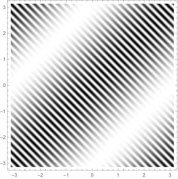
where x=(x1,x2,…,xd)x=(x_{1},x_{2},\dots,x_{d}), which are L2L^{2}-normalized eigenfunctions on (𝕋d,dvol)({\mathbb{T}}^{d},\operatorname{dvol}) with eigenvalue λm\lambda_{m}. See Figure 1 for a plot of the intensities |ψm​(x)|2|\psi_{m}(x)|^{2}.

Refer to caption
Figure 1. Plot of the intensities of |ψm​(x)|2|\psi_{m}(x)|^{2} for m=10m=10 in dimension d=2d=2, where ψm​(x)=cos⁡(m​x1+(m+1)​x2)+cos⁡((m+1)​x1+m​x2).\psi_{m}(x)=\cos(mx_{1}+(m+1)x_{2})+\cos((m+1)x_{1}+mx_{2}).

Squaring out we get

|ψm​(x)|2=1+cos⁡(x1−x2)+cos⁡((2​m+1)​(x1+x2))+12​cos⁡((2​m+2)​x1+2​m​x2)+12​cos⁡(2​m​x1+(2​m+2)​x2)|\psi_{m}(x)|^{2}=1+\cos(x_{1}-x_{2})+\cos((2m+1)(x_{1}+x_{2}))\\ +\frac{1}{2}\cos((2m+2)x_{1}+2mx_{2})+\frac{1}{2}\cos(2mx_{1}+(2m+2)x_{2})

and we wish to average this over the ball B⁡(0,rm)B(0,r_{m}).

For the term cos⁡(x1−x2)\cos(x_{1}-x_{2}), observe that its average over B⁡(0,rm)B(0,r_{m}) tends to 11, because on this shrinking ball, we have |x1−x2|≤2​rm|x_{1}-x_{2}|\leq 2r_{m} and hence cos⁡(x1−x2)=1+O⁡(rm2)\cos(x_{1}-x_{2})=1+O(r_{m}^{2}), so that

1vol⁡(B⁡(0,rm))​∫B⁡(0,rm)cos⁡(x1−x2)​dvol⁡(x)=1+O⁡(rm2)→1,as​rm→0.\frac{1}{\operatorname{vol}(B(0,r_{m}))}\int_{B(0,r_{m})}\cos(x_{1}-x_{2})\operatorname{dvol}(x)=1+O(r_{m}^{2})\to 1,\quad{\rm as}\;r_{m}\to 0\;.

To handle the other three terms, note that if μ∈ℤd\mu\in{\mathbb{Z}}^{d} is any frequency vector, then changing variables we find

1vol⁡(B⁡(0,rm))​∫B⁡(0,rm)cos⁡(⟨μ,x⟩)​dvol⁡(x)=1vol⁡(B⁡(0,1))​∫B⁡(0,1)cos⁡(⟨rm​μ,y⟩)​dvol⁡(y)\ \frac{1}{\operatorname{vol}(B(0,r_{m}))}\int_{B(0,r_{m})}\cos(\langle\mu,x\rangle)\operatorname{dvol}(x)=\frac{1}{\operatorname{vol}(B(0,1))}\int_{B(0,1)}\cos(\langle r_{m}\mu,y\rangle)\operatorname{dvol}(y)

that is we get the Fourier transform of the unit ball at the frequency rm​μr_{m}\mu. As is well known, the Fourier transform of the unit ball decays in all directions:

1vol⁡(B⁡(0,1))​∫B⁡(0,1)cos⁡(⟨ξ,x⟩)​dvol⁡(x)→0,as​|ξ|→∞.\frac{1}{\operatorname{vol}(B(0,1))}\int_{B(0,1)}\cos(\langle\xi,x\rangle)\operatorname{dvol}(x)\to 0,\quad{\rm as}\;|\xi|\to\infty\;.

Therefore, applying this to the frequency vectors μ=(2​m,2​m+2,0→)\mu=(2m,2m+2,\vec{0}), (2​m+2,2​m,0→)(2m+2,2m,\vec{0}) and (2​m+1,2​m+1,0→)(2m+1,2m+1,\vec{0}), which have length |μ|≈m|\mu|\approx m, we get

1vol⁡(B⁡(0,rm))​∫B⁡(0,rm)cos⁡(⟨μ,x⟩)​dvol⁡(x)→0,rm​|μ|→∞.\frac{1}{\operatorname{vol}(B(0,r_{m}))}\int_{B(0,r_{m})}\cos(\langle\mu,x\rangle)\operatorname{dvol}(x)\to 0,\quad r_{m}|\mu|\to\infty\;.

Thus whenever rm→0r_{m}\to 0, with rm⋅m≈rm​λm→∞r_{m}\cdot m\approx r_{m}\sqrt{\lambda_{m}}\to\infty,

1vol⁡(B⁡(0,rm))​∫B⁡(0,rm)|ψm​(x)|2​dvol⁡(x)=2+o⁡(1)\frac{1}{\operatorname{vol}(B(0,r_{m}))}\int_{B(0,r_{m})}|\psi_{m}(x)|^{2}\operatorname{dvol}(x)=2+o(1)

giving our claim. ∎

4. Below the critical radius: r<λ−12​(d−1)r<\lambda^{-\frac{1}{2(d-1)}}

In this section, we detail Bourgain’s argument which gives for balls with radii r<λ−12​(d−1)−o⁡(1)r<\lambda^{-\frac{1}{2(d-1)}-o(1)} that in each eigenspace there is an orthonormal set of eigenfunctions with size exceeding a positive multiple of the dimension of the eigenspace, which consists of eigenfunctions whose L2L^{2} mass is scarce in the ball B⁡(0,r)B(0,r).

Denote

ℰλ={μ∈ℤd:|μ|2=λ},Nλ=#​ℰλ.\mathcal{E}_{\lambda}=\{\mu\in{\mathbb{Z}}^{d}:|\mu|^{2}=\lambda\},\qquad N_{\lambda}=\#\mathcal{E}_{\lambda}\;.
Theorem 4.1 (Bourgain).

Suppose d≥3d\geq 3. Also, if d=3d=3 suppose λ≢0,4,7mod8\lambda\not\equiv 0,4,7\mod 8, and, if d=4d=4 suppose λ\lambda is odd. Then for each such λ\lambda-eigenspace there exists an orthonormal set of eigenfunctions 𝒜⊂{ψλn}λn=λ\mathcal{A}\subset\{\psi_{\lambda_{n}}\}_{\lambda_{n}=\lambda} with size #​𝒜≫Nλ\#\mathcal{A}\gg N_{\lambda} such that for each ψ∈𝒜\psi\in\mathcal{A}

1vol⁡(B⁡(0,r))​∫B⁡(0,r)|ψ⁡(x)|2​dvol⁡(x)→0(λ→∞)\frac{1}{\operatorname{vol}(B(0,r))}\int_{B(0,r)}|\psi(x)|^{2}\operatorname{dvol}(x)\rightarrow 0\qquad(\lambda\rightarrow\infty)

provided that r<λ−12​(d−1)−o⁡(1)r<\lambda^{-\frac{1}{2(d-1)}-o(1)}.

Completing the orthonormal set 𝒜\mathcal{A} in Theorem 4.1 (in any way) gives an ONB of eigenfunctions ℬ\mathcal{B} with the property that a positive proportion of ψ∈ℬ\psi\in\mathcal{B} do not equidistribute within the small balls B⁡(0,r)B(0,r), r<λ12​(d−1)−o⁡(1)r<\lambda^{\frac{1}{2(d-1)}-o(1)}. Hence, the scale achieved in Theorems 1.1 and 1.2 is sharp.

Before detailing Bourgain’s argument we require the following lemma on the distribution of points on spheres. For each point μ∈λ​Sd−1\mu\in\sqrt{\lambda}S^{d-1}, we associate the cap cap⁡(μ;Y)=Ball⁡(μ,Y)∩λ​Sd−1\operatorname{cap}(\mu;Y)=\operatorname{Ball}(\mu,Y)\cap\sqrt{\lambda}S^{d-1} of size YY about μ\mu, where Ball⁡(x,Y)={y∈ℝd:|x−y|≤Y}\operatorname{Ball}(x,Y)=\{y\in\mathbb{R}^{d}:|x-y|\leq Y\}.

Lemma 4.2.

Suppose for a sequence of λ\lambda’s, we are given a finite set 𝒜λ⊂λ​Sd−1\mathcal{A}_{\lambda}\subset\sqrt{\lambda}S^{d-1} of points on the sphere, with cardinality #​𝒜λ→∞\#\mathcal{A}_{\lambda}\to\infty as λ→∞\lambda\to\infty. Let Y=YλY=Y_{\lambda} satisfy Yλ≫λ1/2+o⁡(1)/(#​𝒜λ)1d−1Y_{\lambda}\gg\lambda^{1/2+o(1)}/(\#\mathcal{A}_{\lambda})^{\frac{1}{d-1}}. Then the set 𝒱⊂𝒜λ\mathcal{V}\subset\mathcal{A}_{\lambda} consisting of ν∈𝒜λ\nu\in\mathcal{A}_{\lambda} such that

#⁡(𝒜λ∩cap⁡(ν,Y))≥2\#\left(\mathcal{A}_{\lambda}\cap\operatorname{cap}(\nu,Y)\right)\geq 2

has density one: #​𝒱∼#​𝒜λ\#\mathcal{V}\sim\#\mathcal{A}_{\lambda} as λ→∞\lambda\to\infty.

Proof.

Let

𝒰={μ∈𝒜λ:#⁡(𝒜λ∩cap⁡(μ;Y))<2}.\mathcal{U}=\left\{\mu\in\mathcal{A}_{\lambda}:\#(\mathcal{A}_{\lambda}\cap\operatorname{cap}(\mu;Y))<2\right\}.

We wish to show that #​𝒰=o⁡(#​𝒜λ)\#\mathcal{U}=o(\#\mathcal{A}_{\lambda}).

Each point on the sphere λ​Sd−1\sqrt{\lambda}S^{d-1} is contained in at most one of the caps of size Y/2Y/2 around μ∈𝒰\mu\in\mathcal{U}, because if cap⁡(μ1;Y/2)∩cap⁡(μ2;Y/2)\operatorname{cap}(\mu_{1};Y/2)\cap\operatorname{cap}(\mu_{2};Y/2) is non-empty for distinct μ1≠μ2∈𝒰\mu_{1}\neq\mu_{2}\in\mathcal{U} then μ2∈cap⁡(μ1;Y)\mu_{2}\in\operatorname{cap}(\mu_{1};Y) contradicting the assumption μ2∈𝒰\mu_{2}\in\mathcal{U}. Consequently the caps cap⁡(μ1,Y/2)\operatorname{cap}(\mu_{1};Y/2) and cap⁡(μ1,Y/2)\operatorname{cap}(\mu_{1};Y/2) are disjoint, so that we have

vol⁡(⋃μ∈𝒰cap⁡(μ,Y/2))=∑μ∈𝒰vol⁡(cap⁡(μ,Y/2))≈Yd−1​#​𝒰\operatorname{vol}\Big(\bigcup\limits_{\mu\in\mathcal{U}}\operatorname{cap}(\mu,Y/2)\Big)=\sum_{\mu\in\mathcal{U}}\operatorname{vol}\Big(\operatorname{cap}(\mu,Y/2)\Big)\approx Y^{d-1}\#\mathcal{U}

and also we have the trivial bound

vol(⋃μ∈𝒰cap(μ,Y/2))≤vol(λSd−1)≪dλ(d−1)/2.\operatorname{vol}\Big(\bigcup\limits_{\mu\in\mathcal{U}}\operatorname{cap}(\mu,Y/2)\Big)\leq\operatorname{vol}(\sqrt{\lambda}S^{d-1})\ll_{d}\lambda^{(d-1)/2}\;.

Combining these formulas we obtain

#​𝒰#​𝒜λ≪1#​𝒜λ⋅λ(d−1)/2Yd−1≪λ−o⁡(1)→0\frac{\#\mathcal{U}}{\#\mathcal{A}_{\lambda}}\ll\frac{1}{\#\mathcal{A}_{\lambda}}\cdot\frac{\lambda^{(d-1)/2}}{Y^{d-1}}\ll\lambda^{-o(1)}\to 0

under our assumption on YY, which gives the claim. ∎

Proof of Theorem 4.1.

First observe that if we have two distinct lattice points μ≠μ′∈ℰλ\mu\neq\mu^{\prime}\in\mathcal{E}_{\lambda}, which are close: 0<|μ−μ′|<Mλ0<|\mu-\mu^{\prime}|<M_{\lambda} (we will take Mλ=λ12​(d−1)+o⁡(1)M_{\lambda}=\lambda^{\frac{1}{2(d-1)}+o(1)}), then the eigenfunction

ψμ​(x):=12​(ei​⟨μ,x⟩−ei​⟨μ′,x⟩)\psi_{\mu}(x):=\frac{1}{\sqrt{2}}\Big(e^{i\langle\mu,x\rangle}-e^{i\langle\mu^{\prime},x\rangle}\Big)

fails to equidistribute in the ball B⁡(0,r)B(0,r) centered at the origin for any r=o⁡(Mλ−1)r=o(M_{\lambda}^{-1}). Indeed, for x∈B⁡(0,r)x\in B(0,r)

|ψμ​(x)|2=1−cos⁡(⟨μ−μ′,x⟩)=O⁡((r​|μ−μ′|)2)|\psi_{\mu}(x)|^{2}=1-\cos(\langle\mu-\mu^{\prime},x\rangle)=O\Big((r|\mu-\mu^{\prime}|)^{2}\Big)

and since r​|μ−μ′|≤r​Mλ=o⁡(1)r|\mu-\mu^{\prime}|\leq rM_{\lambda}=o(1), we have

|ψμ​(x)|2=o⁡(1),x∈B⁡(0,r).|\psi_{\mu}(x)|^{2}=o(1),\quad x\in B(0,r)\;.

Therefore

1vol⁡(B⁡(0,r))​∫B⁡(0,r)|ψμ​(x)|2​dvol⁡(x)→0.\frac{1}{\operatorname{vol}(B(0,r))}\int_{B(0,r)}|\psi_{\mu}(x)|^{2}\operatorname{dvol}(x)\to 0\;.

Next we claim that there is a set 𝒮⊂ℰλ\mathcal{S}\subset\mathcal{E}_{\lambda} containing a positive proportion of μ\mu’s (#​𝒮/Nλ≫1\#\mathcal{S}/N_{\lambda}\gg 1) such that :

  • •

    for each μ∈𝒮\mu\in\mathcal{S} there is another lattice point μ′\mu^{\prime} which is close to μ\mu: |μ−μ′|<λ12​(d−1)+o⁡(1)|\mu-\mu^{\prime}|<\lambda^{\frac{1}{2(d-1)}+o(1)};

  • •

    if μ≠ν∈𝒮\mu\neq\nu\in\mathcal{S} are distinct, then the pairs {μ,μ′}\{\mu,\mu^{\prime}\} and {ν,ν′}\{\nu,\nu^{\prime}\} are disjoint, that is ν≠μ′\nu\neq\mu^{\prime} and ν′≠μ,μ′\nu^{\prime}\neq\mu,\mu^{\prime}.

Given this, we form for each μ∈𝒮\mu\in\mathcal{S} the eigenfunction ψμ\psi_{\mu}, and then for μ≠ν∈𝒮\mu\neq\nu\in\mathcal{S} the pairs {μ,μ′}\{\mu,\mu^{\prime}\} and {ν,ν′}\{\nu,\nu^{\prime}\} are disjoint, and so the eigenfunctions ψμ\psi_{\mu} and ψν\psi_{\nu} are orthogonal. This establishes Bourgain’s result Theorem 4.1

It remains to prove the claim. Let Yλ=λ12​(d−1)+o⁡(1)Y_{\lambda}=\lambda^{\frac{1}{2(d-1)}+o(1)}. We construct 𝒮\mathcal{S} as follows: In Lemma 4.2 first take 𝒜λ0=ℰλ\mathcal{A}_{\lambda}^{0}=\mathcal{E}_{\lambda}, and note that under the assumption of the theorem on λ\lambda, we have #​𝒜λ0=Nλ≫λd2−1−o⁡(1)\#\mathcal{A}_{\lambda}^{0}=N_{\lambda}\gg\lambda^{\frac{d}{2}-1-o(1)} (see Section 5.1) so that Yλ≫λ1/2+o⁡(1)/Nλ1d−1Y_{\lambda}\gg\lambda^{1/2+o(1)}/N_{\lambda}^{\frac{1}{d-1}}. Hence by Lemma 4.2 we get a set 𝒱\mathcal{V} of density one. Take some μ∈𝒱\mu\in\mathcal{V}; then there exists μ′∈𝒜λ0\mu^{\prime}\in\mathcal{A}_{\lambda}^{0} such that 0<|μ−μ′|<λ12​(d−1)+o⁡(1)0<|\mu-\mu^{\prime}|<\lambda^{\frac{1}{2(d-1)}+o(1)}. Now remove the pair {μ,μ′}\{\mu,\mu^{\prime}\} from ℰλ\mathcal{E}_{\lambda}, to obtain a smaller set 𝒜λ1=𝒜λ0\{μ,μ′}\mathcal{A}_{\lambda}^{1}=\mathcal{A}_{\lambda}^{0}\backslash\{\mu,\mu^{\prime}\}, and repeat this process (12−o⁡(1))​Nλ(\frac{1}{2}-o(1))N_{\lambda} times, at each time getting a non-empty remainder set 𝒜λj\mathcal{A}_{\lambda}^{j}, of size #​𝒜λj≫Nλ\#\mathcal{A}_{\lambda}^{j}\gg N_{\lambda}, so that still Yλ≫λ1/2+o⁡(1)/#​𝒜λjY_{\lambda}\gg\lambda^{1/2+o(1)}/\#\mathcal{A}_{\lambda}^{j} and we can continue to invoke Lemma 4.2.

We obtain (12−o⁡(1))​Nλ(\frac{1}{2}-o(1))N_{\lambda} resulting pairs, which by construction are close and disjoint. In this way we obtain a set 𝒮\mathcal{S} of density 12−o⁡(1)\frac{1}{2}-o(1) with the desired properties. ∎

5. Results for individual eigenspaces

5.1. Arithmetic background

We denote by Rd​(n)R_{d}(n) the number of representations of nn as a sum of dd squares. This is the dimension of the nn-eigenspace of the Laplacian on 𝕋d\mathbb{T}^{d}. For d=4d=4, Jacobi’s four square theorem says that R4​(n)=8​∑d|n,4∤ddR_{4}(n)=8\sum_{d\mid n,4\nmid d}d so that R4​(n)≪n1+o⁡(1)R_{4}(n)\ll n^{1+o(1)} and for nn odd we have a lower bound R4​(n)≥8​nR_{4}(n)\geq 8n. For d=3d=3, we have R3​(n)≪n1/2+o⁡(1)R_{3}(n)\ll n^{1/2+o(1)} and Siegel’s theorem says that for n≠0,4,7mod8n\neq 0,4,7\mod 8, we have a lower bound R3​(n)≫n1/2−o⁡(1)R_{3}(n)\gg n^{1/2-o(1)}. When d≥5d\geq 5, a classical result of Hardy and Ramanujan gives Rd​(n)≈nd/2−1R_{d}(n)\approx n^{d/2-1}. For more details on these bounds including more precise formulas see e.g.[16, Chapter 11], [8].

For n,t≥1n,t\geq 1 let Ad​(n,t)A_{d}(n,t) denote the number of representations of the positive definite binary quadratic form

Q⁡(x,y)=n​x2+2​t​x​y+n​y2Q(x,y)=nx^{2}+2txy+ny^{2}

as a sum of squares of dd linear forms. That is,

Ad​(n,t)=#⁡{(μ,ν)∈ℤd×ℤd:∑j=1d(μj​x+νj​y)2=Q⁡(x,y)}.A_{d}(n,t)=\#\left\{(\mu,\nu)\in\mathbb{Z}^{d}\times\mathbb{Z}^{d}:\sum_{j=1}^{d}(\mu_{j}x+\nu_{j}y)^{2}=Q(x,y)\right\}.

where xx, yy are indeterminates. Equivalently,

Ad​(n,t)=#⁡{(μ,ν)∈ℤd×ℤd:|μ|2=|ν|2=n​ and ​⟨μ,ν⟩=t}.A_{d}(n,t)=\#\left\{(\mu,\nu)\in\mathbb{Z}^{d}\times\mathbb{Z}^{d}:|\mu|^{2}=|\nu|^{2}=n\text{ and }\langle\mu,\nu\rangle=t\right\}\;.

The number of representations of quadratic forms by quadratic forms has been widely studied. This generalizes the classical problem of representing integers by quadratic forms and for a survey of results on these problems see [30]. The study of the more specific case of representing a quadratic form by a sum of squares of linear forms dates back to at least Mordell who studied the criteria for which such a representation exists in a small number of variables (such a representation always exists if the number of variables is sufficiently large). In the case d=3d=3 Venkov [33] [34, Chapter 4.16] and Pall [25, 26] studied A3​(n,t)A_{3}(n,t), obtaining an exact, but complicated formula for it. From this one can deduce the following useful bound:

Lemma 5.1.

If |t|<n|t|<n then

A3​(n,t)≪gcd⁡(n,t)1/2​no⁡(1).A_{3}(n,t)\ll\gcd(n,t)^{1/2}n^{o(1)}.

This kind of bound was stated and used by Linnik [20], who omitted the factor of gcd⁡(n,t)1/2\gcd(n,t)^{1/2}. A correct version was given by Pall [25, §7], [26, Theorem 4], see also [3, Proposition 2.2].

In the case d=4d=4, Pall and Taussky [27] established an exact formula for A4​(n,t)A_{4}(n,t). The relevant case for us will be when nn is odd, in this case their formulas states the following.

Lemma 5.2.

If nn is odd and |t|<n|t|<n then setting e:=gcd⁡(n,t)e:=\gcd(n,t), we have

A4(n,t)=∑h|eR4(h)⋅#{ν∈ℤ3:|ν|2=n2−t2,gcd(ν1,ν2,ν3,e)=h}.A_{4}(n,t)=\sum_{h|e}R_{4}(h)\cdot\#\{\nu\in\mathbb{Z}^{3}:|\nu|^{2}=n^{2}-t^{2},\gcd(\nu_{1},\nu_{2},\nu_{3},e)=h\}\;.

In particular, for nn odd Lemma 5.2 gives

(5.1) A4​(n,t)≥8⋅R3​(n2−t2).A_{4}(n,t)\geq 8\cdot R_{3}(n^{2}-t^{2}).

with equality holding if gcd⁡(n,t)=1\gcd(n,t)=1. This is seen by using R4​(h)≥8R_{4}(h)\geq 8 for odd hh and noting that every ν\nu with |ν|2=n2−t2|\nu|^{2}=n^{2}-t^{2}, will satisfy gcd⁡(ν1,ν2,ν3,e)=h\gcd(\nu_{1},\nu_{2},\nu_{3},e)=h for some h|eh\mid e.

To get an upper bound for A4​(n,t)A_{4}(n,t), first note that for |t|<n|t|<n and h|eh|e

#{ν∈ℤ3:|ν|2=n2−t2,gcd(ν1,ν2,ν3,e)=h}≤R3​(n2−t2h2)≪(n2−t2h2)1/2+o⁡(1),\#\{\nu\in\mathbb{Z}^{3}:|\nu|^{2}=n^{2}-t^{2},\gcd(\nu_{1},\nu_{2},\nu_{3},e)=h\}\\ \qquad\qquad\leq R_{3}\left(\frac{n^{2}-t^{2}}{h^{2}}\right)\ll\left(\frac{n^{2}-t^{2}}{h^{2}}\right)^{1/2+o(1)},

where in the last step we used the bound R3​(m)≪m1/2+o⁡(1)R_{3}(m)\ll m^{1/2+o(1)}. Now use this estimate in Lemma 5.2 along with the bounds R4​(h)≪h1+o⁡(1)R_{4}(h)\ll h^{1+o(1)} and ∑h|e1≪eo⁡(1)\sum_{h\mid e}1\ll e^{o(1)} to get for nn odd and |t|<n|t|<n that

(5.2) A4​(n,t)≪n1/2+o⁡(1)​(n−t)1/2,A_{4}(n,t)\ll n^{1/2+o(1)}(n-t)^{1/2},

uniformly for |t|<n|t|<n.

5.2. L1L^{1} discrepancy for each λ\lambda-eigenspace

For a∈C⁡(𝕋d)a\in C({\mathbb{T}}^{d}) define the localized L1L^{1} discrepancy

V1loc​(a,λ)=∑λn=λ|⟨a​ψn,ψn⟩−⟨a,1⟩|.V_{1}^{\operatorname{loc}}(a,\lambda)=\sum_{\lambda_{n}=\lambda}|\langle a\psi_{n},\psi_{n}\rangle-\langle a,1\rangle|.
Lemma 5.3.

Suppose T≤2​λT\leq\sqrt{2\lambda}. Then

∑1≤|ζ|≤TV1loc​(eζ,λ)≤∑λ−T2/2≤t≤λ−1Ad​(λ,t).\sum_{1\leq|\zeta|\leq T}V_{1}^{\operatorname{loc}}(e_{\zeta},\lambda)\leq\sum_{\lambda-T^{2}/2\leq t\leq\lambda-1}A_{d}(\lambda,t).
Proof.

Applying Lemma 2.2 gives

∑1≤|ζ|≤TV1loc​(eζ,λ)≤∑2≤|ζ|2≤T2#⁡{μ:|μ|2=λ=|μ+ζ|2}.\sum_{1\leq|\zeta|\leq T}V_{1}^{\operatorname{loc}}(e_{\zeta},\lambda)\leq\sum_{\begin{subarray}{c}2\leq|\zeta|^{2}\leq T^{2}\end{subarray}}\#\left\{\mu:|\mu|^{2}=\lambda=|\mu+\zeta|^{2}\right\}\;.

(Note we can ignore ζ\zeta with |ζ|2|\zeta|^{2} odd, since for these ⟨eζ​ψn,ψn⟩=0\langle e_{\zeta}\psi_{n},\psi_{n}\rangle=0.) Next, observe that

∑2≤|ζ|2≤T2#⁡{μ:|μ|2=λ=|μ+ζ|2}=∑2≤ℓ≤T2∑μ,ν∈ℤd|μ|2=λ=|ν|2|μ−ν|2=ℓ1.\begin{split}\sum_{\begin{subarray}{c}2\leq|\zeta|^{2}\leq T^{2}\end{subarray}}\#\left\{\mu:|\mu|^{2}=\lambda=|\mu+\zeta|^{2}\right\}=&\sum_{2\leq\ell\leq T^{2}}\sum_{\begin{subarray}{c}\mu,\nu\in\mathbb{Z}^{d}\\ |\mu|^{2}=\lambda=|\nu|^{2}\\ |\mu-\nu|^{2}=\ell\end{subarray}}1.\end{split}

For |μ|2=|ν|2=λ|\mu|^{2}=|\nu|^{2}=\lambda we have |μ−ν|2=ℓ|\mu-\nu|^{2}=\ell iff ⟨μ,ν⟩=(λ−ℓ/2)\langle\mu,\nu\rangle=(\lambda-\ell/2). Hence,

∑2≤ℓ≤T2∑μ,ν∈ℤd|μ|2=λ=|ν|2|μ−ν|2=ℓ1=∑λ−T2/2≤t≤λ−1Ad​(λ,t).\sum_{2\leq\ell\leq T^{2}}\sum_{\begin{subarray}{c}\mu,\nu\in\mathbb{Z}^{d}\\ |\mu|^{2}=\lambda=|\nu|^{2}\\ |\mu-\nu|^{2}=\ell\end{subarray}}1=\sum_{\lambda-T^{2}/2\leq t\leq\lambda-1}A_{d}(\lambda,t).

∎

5.3. Proof of Theorem 1.2

Suppose that d=3d=3 or d=4d=4. For d=3d=3 suppose λ≢0,4,7(mod8)\lambda\not\equiv 0,4,7\pmod{8}, so the dimension of the λ\lambda-eigenspace, NλN_{\lambda}, is ≈λ1/2±o⁡(1)\approx\lambda^{1/2\pm o(1)}; if d=4d=4 suppose λ\lambda is odd so that λ≪Nλ≪λ1+o⁡(1)\lambda\ll N_{\lambda}\ll\lambda^{1+o(1)}. Let

ℬλ={B⁡(y,r)⊂𝕋d:r≥λ−θ1}\mathcal{B}_{\lambda}=\left\{B(y,r)\subset{\mathbb{T}}^{d}:r\geq\lambda^{-\theta_{1}}\right\}

for θ1\theta_{1} to be determined later. As in the proof of Theorem 1.1 we take bn,y±b_{n,y}^{\pm} to be Beurling-Selberg polynomials which majorize and minorize the indicator function of the ball B⁡(y,r)B(y,r) with r≥λn−θ1=λ−θ1r\geq\lambda_{n}^{-\theta_{1}}=\lambda^{-\theta_{1}}. We take the lengths of the polynomials bn,y±b_{n,y}^{\pm} to be Tn=λnθ2=λθ2T_{n}=\lambda_{n}^{\theta_{2}}=\lambda^{\theta_{2}} with θ2>θ1\theta_{2}>\theta_{1}. Given an orthonormal basis {ψn}λn=λ\{\psi_{n}\}_{\lambda_{n}=\lambda} of the λ\lambda-eigenspace define

𝒮λ±={λn=λ:supB⁡(y,r)∈ℬλ|∫𝕋dbn,y±​(x)​|ψn​(x)|2​dvol⁡(x)∫𝕋dbn,y±​(x)​dvol⁡(x)−1|≥λ−δ}.\mathcal{S}_{\lambda}^{\pm}=\left\{\lambda_{n}=\lambda:\sup_{B(y,r)\in\mathcal{B}_{\lambda}}\bigg|\frac{\int_{\mathbb{T}^{d}}b_{n,y}^{\pm}(x)|\psi_{n}(x)|^{2}\,\operatorname{dvol}(x)}{\int_{\mathbb{T}^{d}}b_{n,y}^{\pm}(x)\,\,\operatorname{dvol}(x)}-1\bigg|\geq\lambda^{-\delta}\right\}.

Using Lemma 5.3 along with the bound b^n,y±≪rd\widehat{b}_{n,y}^{\pm}\ll r^{d} given by Lemma 2.5 (iv) (which holds uniformly in yy), we get from Chebyshev’s inequality as in the proof of Theorem 1.1 that

#​𝒮λ±Nλ≪1λd2−1−2​δ​∑1≤|ζ|≤λθ2∑λn=λ|⟨eζ​ψn,ψn⟩|​supB⁡(y,r)∈ℬλ|b^n,y±​(ζ)b^n,y±​(0)|≪1λd2−1−2​δ​∑1≤|ζ|≤λθ2V1loc​(eζ,λ)≪1λd2−1−2​δ​∑λ−λ2​θ2/2≤t<λAd​(λ,t).\begin{split}\frac{\#\mathcal{S}_{\lambda}^{\pm}}{N_{\lambda}}&\ll\frac{1}{\lambda^{\frac{d}{2}-1-2\delta}}\sum_{1\leq|\zeta|\leq\lambda^{\theta_{2}}}\sum_{\lambda_{n}=\lambda}|\langle e_{\zeta}\psi_{n},\psi_{n}\rangle|\sup_{B(y,r)\in\mathcal{B}_{\lambda}}\left|\frac{\widehat{b}_{n,y}^{\pm}(\zeta)}{\widehat{b}_{n,y}^{\pm}(0)}\right|\\ &\ll\frac{1}{\lambda^{\frac{d}{2}-1-2\delta}}\sum_{1\leq|\zeta|\leq\lambda^{\theta_{2}}}V_{1}^{\operatorname{loc}}(e_{\zeta},\lambda)\\ &\ll\frac{1}{\lambda^{\frac{d}{2}-1-2\delta}}\sum_{\lambda-\lambda^{2\theta_{2}}/2\leq t<\lambda}A_{d}(\lambda,t)\;.\end{split}

Since we assume d=3d=3 and λ≢0,4,7(mod8)\lambda\not\equiv 0,4,7\pmod{8} or d=4d=4 and λ\lambda odd, combining Lemma 5.1 and (5.2) gives

Ad​(λ,t)≪λ(d−3)/2+o⁡(1)​gcd⁡(λ,t)​(λ−t)(d−3)/2.A_{d}(\lambda,t)\ll\lambda^{(d-3)/2+o(1)}\gcd(\lambda,t)(\lambda-t)^{(d-3)/2}.

Thus,

∑λ−λ2​θ2/2≤t<λAd​(λ,t)≪λ(d−3)/2+θ2​(d−3)+o⁡(1)​∑λ−λ2​θ2/2≤t<λgcd⁡(λ,t)≪λ(d−3)/2+θ2​(d−3)+o⁡(1)​∑e|λe​∑λ−λ2​θ2/2e≤t0<λ/e1≪λ(d−3)/2+θ2​(d−1)+o⁡(1),\begin{split}\sum_{\lambda-\lambda^{2\theta_{2}}/2\leq t<\lambda}A_{d}(\lambda,t)\ll&\lambda^{(d-3)/2+\theta_{2}(d-3)+o(1)}\sum_{\lambda-\lambda^{2\theta_{2}}/2\leq t<\lambda}\operatorname{gcd}(\lambda,t)\\ \ll&\lambda^{(d-3)/2+\theta_{2}(d-3)+o(1)}\sum_{e|\lambda}e\sum_{\begin{subarray}{c}\frac{\lambda-\lambda^{2\theta_{2}}/2}{e}\leq t_{0}<\lambda/e\end{subarray}}1\\ \ll&\lambda^{(d-3)/2+\theta_{2}(d-1)+o(1)},\end{split}

where in the last step we bounded the inner sum as O⁡(λ2​θ2/e)O(\lambda^{2\theta_{2}}/e) since if λ2​θ2/(2​e)<1\lambda^{2\theta_{2}}/(2e)<1 then the sum is empty. Collecting estimates gives

#​𝒮λ±Nλ≪λθ2​(d−1)−12+3​δ,\frac{\#\mathcal{S}_{\lambda}^{\pm}}{N_{\lambda}}\ll\lambda^{\theta_{2}(d-1)-\frac{1}{2}+3\delta},

which tends to zero if θ1<θ2<12​(d−1)−3​δ\theta_{1}<\theta_{2}<\frac{1}{2(d-1)}-3\delta.

Thus, the subset of the ONB {ψn}λn=λ\{\psi_{n}\}_{\lambda_{n}=\lambda}, which consists of eigenfunctions ψn\psi_{n} with λn∉(Sλ+∪Sλ−)\lambda_{n}\notin\mathcal{(}S_{\lambda}^{+}\cup S_{\lambda}^{-}) has cardinality Nλ​(1+o​(1))N_{\lambda}(1+o(1)) provided θ1<θ2<12​(d−1)−3​δ\theta_{1}<\theta_{2}<\frac{1}{2(d-1)}-3\delta. Repeating the same argument given at the end of the proof of Theorem 1.1 (see equations (2.2), (2.3)) we see that each eigenfunction in this subset satisfies

supB⁡(y,r)∈ℬλ|∫B⁡(y,r)|ψn​(x)|2​dvol⁡(x)−vol⁡(B⁡(y,r))|≪rd​λ−δ+rd​λθ1−θ2.\sup_{B(y,r)\in\mathcal{B}_{\lambda}}\left|\int_{B(y,r)}|\psi_{n}(x)|^{2}\operatorname{dvol}(x)-\operatorname{vol}(B(y,r))\right|\ll r^{d}\lambda^{-\delta}+r^{d}\lambda^{\theta_{1}-\theta_{2}}\;.

∎

Remark 5.4.

Our argument reduces the problem of small scale quantum ergodicity to a lattice point estimate, which can be rephrased in terms of statistics of lattice points in caps: For each lattice point ν∈ℰλ={μ∈ℤd:|μ|2=λ}\nu\in\mathcal{E}_{\lambda}=\{\mu\in{\mathbb{Z}}^{d}:|\mu|^{2}=\lambda\}, let

(5.3) 𝔫⁡(ν,Y)=#⁡(ℰλ∩cap⁡(ν,Y))−1=#⁡{μ∈ℰλ:0<|μ−ν|≤Y}{\mathfrak{n}}(\nu,Y)=\#(\mathcal{E}_{\lambda}\cap\operatorname{cap}(\nu,Y))-1=\#\{\mu\in\mathcal{E}_{\lambda}:0<|\mu-\nu|\leq Y\}

be the number of other lattice points in a cap of size YY about ν\nu. In fact we actually show that in any dimension d≥3d\geq 3 if

1Nλ​∑|ν|2=λ𝔫⁡(ν,Y)→0,as​λ→∞\frac{1}{N_{\lambda}}\sum_{|\nu|^{2}=\lambda}{\mathfrak{n}}(\nu,Y)\to 0,\quad{\rm as}\;\lambda\to\infty

then the assertion of Theorem 1.2 holds in dimension dd at scales r>Y−1+o⁡(1)r>Y^{-1+o(1)} (we also assume here that λ≢0,4,7(mod8)\lambda\not\equiv 0,4,7\pmod{8} if d=3d=3 and λ\lambda is odd if d=4d=4, for d≥5d\geq 5 no such restrictions are needed). That is, given the above, small scale quantum ergodicity holds in dimension dd at scales above r>Y−1+o⁡(1)r>Y^{-1+o(1)} on every such λ\lambda-eigenspace.

6. Massive irregularities

In this section we are concerned with the existence of a sequence of eigenfunctions ψλ\psi_{\lambda} for which the proportion of the L2L^{2} mass of ψλ\psi_{\lambda} within small balls becomes arbitrarily large as λ→∞\lambda\rightarrow\infty. For d=4d=4 we show the existence of such a sequence of eigenfunctions ψλ\psi_{\lambda} for balls with radii rλ≤λ−1/6−o(1)r_{\lambda}\leq\lambda^{-1/6-o(1)}. On the other hand, for d=2d=2 we are able to rule out this behavior for balls with radii that shrink sufficiently slowly.

6.1. Blowup for d=4d=4

Let

(6.1) ψλ​(x)=1Nλ​∑|μ|2=λeμ​(x).\psi_{\lambda}(x)=\frac{1}{\sqrt{N_{\lambda}}}\sum_{|\mu|^{2}=\lambda}e_{\mu}(x)\;.

We show that at small scales the L2L^{2} mass of ψλ\psi_{\lambda} blows up in dimension d=4d=4.

Theorem 6.1.

Let ψm=ψλm\psi_{m}=\psi_{\lambda_{m}} be as given in (6.1) in dimension d=4d=4. Then along the sequence of odd eigenvalues λm\lambda_{m} we have for any sequence of radii rm<λm−1/6−o(1)r_{m}<\lambda_{m}^{-1/6-o(1)},

limm→∞1vol⁡(B⁡(0,rm))​∫B⁡(0,rm)|ψm​(x)|2​dvol⁡(x)=∞.\lim_{m\to\infty}\frac{1}{\operatorname{vol}(B(0,r_{m}))}\int_{B(0,r_{m})}|\psi_{m}(x)|^{2}\operatorname{dvol}(x)=\infty.

Note that the result is trivial for r=o(λ−1/2)r=o(\lambda^{-1/2}), because then for x∈B⁡(0,r)x\in B(0,r) we can replace ψλ​(x)∼ψ⁡(0)=Nλ\psi_{\lambda}(x)\sim\psi(0)=\sqrt{N_{\lambda}} and then the average of |ψλ​(x)|2|\psi_{\lambda}(x)|^{2} over the ball B⁡(0,r)B(0,r) will be large. This also implies that for r≥ελ−1/2r\geq\varepsilon\lambda^{-1/2} with ε>0\varepsilon>0 sufficiently small

1vol⁡(B⁡(0,r))​∫B⁡(0,r)|ψλ​(x)|2​dvol⁡(x)≥1vol⁡(B⁡(0,r))∫B(0,ελ−1/2)|ψλ(x)|2dvol(x)≫Nλrd⋅εdλ−d/2\begin{split}\frac{1}{\operatorname{vol}(B(0,r))}\int_{B(0,r)}|\psi_{\lambda}(x)|^{2}\operatorname{dvol}(x)\geq&\frac{1}{\operatorname{vol}(B(0,r))}\int_{B(0,\varepsilon\lambda^{-1/2})}|\psi_{\lambda}(x)|^{2}\operatorname{dvol}(x)\\ \gg&\frac{N_{\lambda}}{r^{d}}\cdot\varepsilon^{d}\lambda^{-d/2}\end{split}

in every dimension d≥2d\geq 2. Recall for d≥3d\geq 3, Nλ≫λd2−1−o⁡(1)N_{\lambda}\gg\lambda^{\frac{d}{2}-1-o(1)} provided that λ\lambda is odd if d=4d=4 and if d=3d=3, λ≢0,4,7(mod8)\lambda\not\equiv 0,4,7\pmod{8}. For such λ\lambda the RHS tends to infinity for rλ≤λ−1d−o⁡(1)r_{\lambda}\leq\lambda^{-\frac{1}{d}-o(1)}. Theorem 6.1 shows that massive irregularities extend beyond this trivial regime.

For T≤2​λT\leq\sqrt{2\lambda} let

Sd​(λ,T)=∑λ−T2/2≤t<λAd​(λ,t)S_{d}(\lambda,T)=\sum_{\lambda-T^{2}/2\leq t<\lambda}A_{d}(\lambda,t)

and note that in the proof of Lemma 5.3 we saw that

(6.2) Sd​(λ,T)=∑2≤|ζ|2≤T2#⁡{μ:|μ|2=λ=|μ+ζ|2}.S_{d}(\lambda,T)=\sum_{2\leq|\zeta|^{2}\leq T^{2}}\#\{\mu:|\mu|^{2}=\lambda=|\mu+\zeta|^{2}\}.
Lemma 6.2.

Let ψλ\psi_{\lambda} be as in (6.1). Suppose that rλ→0r_{\lambda}\rightarrow 0 as λ→∞\lambda\rightarrow\infty. Then for any dimension d≥2d\geq 2

1vol⁡B⁡(0,rλ)​∫B⁡(0,rλ)|ψλ​(x)|2​dvol⁡(x)≫1+Sd​(λ,rλ−1+o⁡(1))Nλ.\frac{1}{\operatorname{vol}B(0,r_{\lambda})}\int_{B(0,r_{\lambda})}|\psi_{\lambda}(x)|^{2}\,\operatorname{dvol}(x)\gg\frac{1+S_{d}(\lambda,r_{\lambda}^{-1+o(1)})}{N_{\lambda}}.
Remark 6.3.

The RHS is bounded below by the mean value

1Nλ​∑|ν|2=λ𝔫⁡(ν,rλ−1+o⁡(1))\frac{1}{N_{\lambda}}\sum_{|\nu|^{2}=\lambda}{\mathfrak{n}}(\nu,r_{\lambda}^{-1+o(1)})

of the other lattice points in caps of size rλ−1+o⁡(1)r_{\lambda}^{-1+o(1)}, where 𝔫⁡(ν,Y){\mathfrak{n}}(\nu,Y) is as defined in (5.3). So if this tends to infinity then the conclusion of Theorem 6.1 holds in dimension dd at scales rλr_{\lambda}.

Proof.

We first construct an auxiliary smooth minorant of 𝟏B⁡(0,rλ)​(x)\mathbf{1}_{B(0,r_{\lambda})}(x) on the torus. Let f∈C0∞​(ℝ)f\in C_{0}^{\infty}(\mathbb{R}) be a nonzero function such that 0≤f⁡(x)≤10\leq f(x)\leq 1 and supp⁡f=[−12,12]\operatorname{supp}f=[-\tfrac{1}{2},\tfrac{1}{2}]. Let g:ℝd→ℝg:\mathbb{R}^{d}\rightarrow\mathbb{R} be given by g⁡(x)=f⁡(|x|)g(x)=f(|x|) and define Frλ:𝕋d→ℝF_{r_{\lambda}}:\mathbb{T}^{d}\to{\mathbb{R}} by

Frλ​(x)=∑n∈ℤd(g∗g)​(x+2​π​nrλ).F_{r_{\lambda}}(x)=\sum_{n\in\mathbb{Z}^{d}}(g\ast g)\left(\frac{x+2\pi n}{r_{\lambda}}\right)\;.

Observe that

(g∗g)​(y)=∫ℝdf⁡(|x|)​f​(|y−x|)​𝑑x<1.(g\ast g)(y)=\int_{\mathbb{R}^{d}}f(|x|)f(|y-x|)dx<1.

Also, for |y|≥1|y|\geq 1

0≤(g∗g)​(y)≤∫|y−x|<12,|x|<121​𝑑x=0.0\leq(g\ast g)(y)\leq\int_{|y-x|<\frac{1}{2},|x|<\frac{1}{2}}1\;dx=0.

It follows that 𝟏B⁡(0,1)​(x)≥(g∗g)​(x)≥0\mathbf{1}_{B(0,1)}(x)\geq(g\ast g)(x)\geq 0. Write

ℱ⁡(g∗g)​(ξ)=∫ℝd(g∗g)​(x)​e−ξ​(x)​d​x(2​π)d=|∫ℝdg⁡(x)​e−ξ​(x)​d​x(2​π)d|2\mathcal{F}(g\ast g)(\xi)=\int_{\mathbb{R}^{d}}(g\ast g)(x)e_{-\xi}(x)\,\frac{dx}{(2\pi)^{d}}=\left|\int_{\mathbb{R}^{d}}g(x)e_{-\xi}(x)\,\frac{dx}{(2\pi)^{d}}\right|^{2}

and note by Poisson summation

Frλ​(x)=∑n∈ℤd(g∗g)​(x+2​π​nrλ)=rλd​∑ζ∈ℤdℱ⁡(g∗g)​(rλ​ζ)​eζ​(x).\begin{split}F_{r_{\lambda}}(x)=\sum_{n\in\mathbb{Z}^{d}}(g\ast g)\left(\frac{x+2\pi n}{r_{\lambda}}\right)=&r_{\lambda}^{d}\sum_{\zeta\in\mathbb{Z}^{d}}\mathcal{F}(g\ast g)(r_{\lambda}\zeta)e_{\zeta}(x).\end{split}

Hence, Frλ:𝕋d→ℝF_{r_{\lambda}}:\mathbb{T}^{d}\rightarrow\mathbb{R} is a smooth minorant of 𝟏B⁡(0,rλ)​(x)\mathbf{1}_{B(0,r_{\lambda})}(x) and has non-negative Fourier coefficients. Also, observe that ℱ⁡(g∗g)​(ξ)=ℱ⁡(g∗g)​(0)+O⁡(|ξ|)\mathcal{F}(g\ast g)(\xi)=\mathcal{F}(g\ast g)(0)+O(|\xi|). From these estimates we get that

∫B⁡(0,rλ)|ψλ​(x)|2dvol⁡(x)≥∫𝕋dFrλ​(x)​|ψλ​(x)|2​dvol⁡(x)=rλdNλ​∑ζ∈ℤdℱ⁡(g∗g)​(rλ​ζ)​#​{μ:|μ|2=λ=|μ+ζ|2}≥rλd2​Nλ​ℱ​(g∗g)​(0)​(1+∑0≠|ζ|≤rλ−1+o⁡(1)#⁡{μ:|μ|2=λ=|μ+ζ|2})\begin{split}\int_{B(0,r_{\lambda})}|\psi_{\lambda}(x)|^{2}\,&\operatorname{dvol}(x)\geq\int_{\mathbb{T}^{d}}F_{r_{\lambda}}(x)|\psi_{\lambda}(x)|^{2}\,\operatorname{dvol}(x)\\ =&\frac{r_{\lambda}^{d}}{N_{\lambda}}\sum_{\zeta\in\mathbb{Z}^{d}}\mathcal{F}(g\ast g)(r_{\lambda}\zeta)\#\{\mu:|\mu|^{2}=\lambda=|\mu+\zeta|^{2}\}\\ \geq&\frac{r_{\lambda}^{d}}{2N_{\lambda}}\mathcal{F}(g\ast g)(0)\left(1+\sum_{0\neq|\zeta|\leq r_{\lambda}^{-1+o(1)}}\#\{\mu:|\mu|^{2}=\lambda=|\mu+\zeta|^{2}\}\right)\end{split}

by dropping the large frequencies using the non-negativity of ℱ⁡(g∗g)\mathcal{F}(g\ast g) and also noting note that ℱ⁡(g∗g)​(0)=|∫ℝdg⁡(x)​d​x(2​π)d|2>0\mathcal{F}(g\ast g)(0)=\left|\int_{{\mathbb{R}}^{d}}g(x)\frac{dx}{(2\pi)^{d}}\right|^{2}>0. Applying (6.2) to the inner sum completes the proof. ∎

6.2. Proof of Theorem 6.1

By Lemma 6.2 it suffices to show that for odd values of λ→∞\lambda\rightarrow\infty such that for any sequence rλ≪λ−16−o⁡(1)r_{\lambda}\ll\lambda^{-\frac{1}{6}-o(1)}, we have

S4​(λ,rλ−1+o⁡(1))/R4​(λ)→∞.S_{4}(\lambda,r_{\lambda}^{-1+o(1)})/R_{4}(\lambda)\rightarrow\infty\;.

By definition, if T=r−1+o⁡(1)T=r^{-1+o(1)},

S4​(λ,T)=∑0<λ−t≤T2/2A4​(λ,t)≥∑0<λ−t≤T2/2t​evenA4​(λ,t).\begin{split}S_{4}(\lambda,T)&=\sum_{0<\lambda-t\leq T^{2}/2}A_{4}(\lambda,t)\\ &\geq\sum_{\begin{subarray}{c}0<\lambda-t\leq T^{2}/2\\ t\;{\rm even}\end{subarray}}A_{4}(\lambda,t)\;.\end{split}

We now assume r>λ−1/2r>\lambda^{-1/2} so that |t|<λ|t|<\lambda. Applying (5.1) for odd λ\lambda we have A4​(λ,t)≥8​R3​(λ2−t2)A_{4}(\lambda,t)\geq 8R_{3}(\lambda^{2}-t^{2}) so that

S4​(λ,T)≥∑0<λ−t≤T2/2t​evenR3​(λ2−t2).S_{4}(\lambda,T)\geq\sum_{\begin{subarray}{c}0<\lambda-t\leq T^{2}/2\\ t\;{\rm even}\end{subarray}}R_{3}(\lambda^{2}-t^{2})\;.

Recall that if n≠0,4,7(mod8)n\neq 0,4,7\pmod{8} then Siegel’s theorem gives R3​(n)≫n12−o⁡(1)R_{3}(n)\gg n^{\frac{1}{2}-o(1)}. Now if λ\lambda is odd and tt is even then λ2−t2=1,5(mod8)\lambda^{2}-t^{2}=1,5\pmod{8} and in particular Siegel’s theorem implies

R3​(λ2−t2)≫(λ2−t2)12−o⁡(1)≫λ12−o⁡(1)​(λ−t)12.R_{3}(\lambda^{2}-t^{2})\gg(\lambda^{2}-t^{2})^{\frac{1}{2}-o(1)}\gg\lambda^{\frac{1}{2}-o(1)}(\lambda-t)^{\frac{1}{2}}\;.

Hence we find

S4​(λ,T)≫λ12−o⁡(1)​∑0<λ−t≤T2/2t​even(λ−t)12=λ12−o⁡(1)​∑1≤m≤T2/2m​oddm1/2≫λ12−o⁡(1)​T3.\begin{split}S_{4}(\lambda,T)\gg&\lambda^{\frac{1}{2}-o(1)}\sum_{\begin{subarray}{c}0<\lambda-t\leq T^{2}/2\\ t\;{\rm even}\end{subarray}}(\lambda-t)^{\frac{1}{2}}\\ =&\lambda^{\frac{1}{2}-o(1)}\sum_{\begin{subarray}{c}1\leq m\leq T^{2}/2\\ m\;{\rm odd}\end{subarray}}m^{1/2}\gg\lambda^{\frac{1}{2}-o(1)}T^{3}.\end{split}

Hence for T≈r−1+o⁡(1)T\approx r^{-1+o(1)} with λ−1/2<r≪λ−1/6+o(1)\lambda^{-1/2}<r\ll\lambda^{-1/6+o(1)}

S4​(λ,r−1+o⁡(1))≫λ12−o⁡(1)​r−3.S_{4}(\lambda,r^{-1+o(1)})\gg\lambda^{\frac{1}{2}-o(1)}r^{-3}\;.

Since R4​(λ)≪λ1+o⁡(1)R_{4}(\lambda)\ll\lambda^{1+o(1)}, we find that along the sequence of odd integers

S4​(λ,rλ−1+o⁡(1))R4​(λ)≫λ−1/2−o(1)r−3→∞\frac{S_{4}(\lambda,r_{\lambda}^{-1+o(1)})}{R_{4}(\lambda)}\gg\lambda^{-1/2-o(1)}r^{-3}\rightarrow\infty

for rλ≪λ−16−o⁡(1)r_{\lambda}\ll\lambda^{-\frac{1}{6}-o(1)}.

∎

6.3. Ruling out blowup for d=2d=2 at certain scales

The construction of massive irregularities in the previous section used some features particular to high dimensions. In fact for d=2d=2, we can rule out the existence of this behavior at scales that are not too small, and expect that massive irregularities do not exist at all scales that are at least slightly above the Planck scale. More precisely, if d=2d=2 then for every eigenfunction ψλ\psi_{\lambda} we will prove that the proportion of L2L^{2} mass inside balls with radii rλ>λ−1/4+o(1)r_{\lambda}>\lambda^{-1/4+o(1)} is bounded and we expect this should be true as long as rλ>λ−1/2+o(1)r_{\lambda}>\lambda^{-1/2+o(1)}.

Proposition 6.4.

Let ψλ​(x)\psi_{\lambda}(x) be an L2​(𝕋2,dvol)L^{2}({\mathbb{T}}^{2},\operatorname{dvol}) normalized eigenfuction in dimension d=2d=2 with eigenvalue λ\lambda. Then for any ball with radius rλ>λ−1/4+o(1)r_{\lambda}>\lambda^{-1/4+o(1)}

(6.3) supy∈𝕋21vol⁡(B⁡(y,r))​∫B⁡(y,r)|ψλ​(x)|2​dvol⁡(x)≪1.\sup_{y\in{\mathbb{T}}^{2}}\frac{1}{\operatorname{vol}(B(y,r))}\int_{B(y,r)}|\psi_{\lambda}(x)|^{2}\operatorname{dvol}(x)\ll 1.
Proof.

Let by+b_{y}^{+} be the translated Beurling-Selberg polynomial described in the proof of Theorem 1.1 which majorizes the indicator function of B⁡(y,r)B(y,r) on 𝕋2{\mathbb{T}}^{2} with length T=2/rT=2/r, so in particular |b^y+​(ζ)/vol⁡(B⁡(y,r))|≪1\Big|\widehat{b}_{y}^{+}(\zeta)/\operatorname{vol}(B(y,r))\Big|\ll 1, uniformly for y∈𝕋2y\in{\mathbb{T}}^{2}. Write

ψλ​(x)=∑|μ|2=λc⁡(μ)​eμ​(x)\psi_{\lambda}(x)=\sum_{|\mu|^{2}=\lambda}c(\mu)e_{\mu}(x)

and argue as in the proof of Lemma 5.3 to get

1vol⁡(B⁡(y,r))​∫B⁡(y,r)|ψλ​(x)|2​dvol⁡(x)≪1+∑2≤ℓ≤T2∑μ,ν∈ℤ2|μ|2=λ=|ν|2|μ−ν|2=ℓ|c⁡(μ)​c​(ν)|≤1+∑|μ|2=λ|c⁡(μ)|2​∑2≤ℓ≤T2∑|ν|2=λ|μ−ν|2=ℓ1,\begin{split}\frac{1}{\operatorname{vol}(B(y,r))}\int_{B(y,r)}|\psi_{\lambda}(x)|^{2}\operatorname{dvol}(x)\ll&1+\sum_{2\leq\ell\leq T^{2}}\sum_{\begin{subarray}{c}\mu,\nu\in\mathbb{Z}^{2}\\ |\mu|^{2}=\lambda=|\nu|^{2}\\ |\mu-\nu|^{2}=\ell\end{subarray}}|c(\mu)c(\nu)|\\ \leq&1+\sum_{|\mu|^{2}=\lambda}|c(\mu)|^{2}\sum_{2\leq\ell\leq T^{2}}\sum_{\begin{subarray}{c}|\nu|^{2}=\lambda\\ |\mu-\nu|^{2}=\ell\end{subarray}}1,\end{split}

uniformly for y∈𝕋2y\in{\mathbb{T}}^{2}. To bound the inner sum, let

M(R,ρ)=max|μ|=R#{ν∈ℤ2:|μ|=R=|ν|,|μ−ν|≤ρ}M(R,\rho)=\max_{|\mu|=R}\#\{\nu\in{\mathbb{Z}}^{2}:|\mu|=R=|\nu|,\;|\mu-\nu|\leq\rho\}

be the maximal number of lattice points in an arc of size ρ\rho on the circle of radius RR. Note that

∑2≤ℓ≤T2∑|ν|2=λ|μ−ν|2=ℓ1≤M⁡(λ,T)−1.\sum_{2\leq\ell\leq T^{2}}\sum_{\begin{subarray}{c}|\nu|^{2}=\lambda\\ |\mu-\nu|^{2}=\ell\end{subarray}}1\leq M(\sqrt{\lambda},T)-1.

Since T=2/rT=2/r we conclude

supy∈𝕋21vol⁡(B⁡(y,r))​∫B⁡(y,r)|ψλ​(x)|2​dvol⁡(x)≪M⁡(λ,2r).\sup_{y\in{\mathbb{T}}^{2}}\frac{1}{\operatorname{vol}(B(y,r))}\int_{B(y,r)}|\psi_{\lambda}(x)|^{2}\operatorname{dvol}(x)\ll M\left(\sqrt{\lambda},\frac{2}{r}\right).

A result of Cilleruelo and Córdoba [4] states that for any 0<δ<1/20<\delta<1/2,

M(R,R1/2−δ)≪δ1,M(R,R^{1/2-\delta})\ll_{\delta}1\;,

thus (6.3) holds for r>λ−1/4+o(1)r>\lambda^{-1/4+o(1)} as claimed. Moreover, we expect that M(R,R1−δ)≪δ1M(R,R^{1-\delta})\ll_{\delta}1; this would imply that (6.3) holds for rλ>λ−1/2+o(1)r_{\lambda}>\lambda^{-1/2+o(1)}. ∎

References

  • [1] M. V. Berry, Regular and irregular semiclassical wave functions. J.Phys.A, 10, (1977) 2083–91.
  • [2] M. V. Berry, Semiclassical mechanics of regular and irregular motion. Chaotic behavior of deterministic systems (Les Houches, 1981), 171–271, North-Holland, Amsterdam, 1983.
  • [3] J. Bourgain, Z. Rudnick and P. Sarnak. Local statistics of lattice points on the sphere. to appear in Contemporary Mathematics, proceedings of Constructive Functions 2014.
  • [4] J. Cilleruelo and A. Córdoba. Lattice points on ellipses. Duke Math. J. 76 (1994), no.3, 741-750.
  • [5] Y. Colin de Verdière Ergodicité et fonctions propres du laplacien. Comm. Math. Phys. 102 (1985), no. 3, 497–502.
  • [6] B. Eckhardt, S. Fishman, J. Keating, O. Agam, J. Main, and K. Müller, Approach to ergodicity in quantum wave functions, Phys. Rev. E 52 (1995), 5893–5903.
  • [7] M. Feingold and A. Peres, Distribution of matrix elements of chaotic systems, Phys. Rev. A 34 (1986), 591–595.
  • [8] E. Grosswald, Representations of integers as sums of squares. Springer-Verlag, New York, 1985.
  • [9] X. Han Small scale quantum ergodicity in negatively curved manifolds. Nonlinearity 28 (2015), no. 9, 3262–3288.
  • [10] G. Harman, On the Erdös-Turán inequality for balls. Acta Arith. 85 (1998), no. 4, 389-396.
  • [11] A. Hassell. Ergodic billiards that are not quantum unique ergodic. With an appendix by the author and Luc Hillairet. Ann. of Math. (2) 171 (2010), no. 1, 605–619.
  • [12] H. Hezari and G. Rivière, LpL^{p} norms, nodal sets, and quantum ergodicity, to appear in Advances in Mathematics, arXiv:1411.4078 [math.AP].
  • [13] H. Hezari and G. Rivière, Quantitative equidistribution properties of toral eigenfunctions, to appear in the Journal of Spectral Theory. arXiv:1503.02794 [math.AP].
  • [14] J. Holt, On a form of the Erdös-Turán inequality. Acta. Arith. 74 (1996), no. 1, 61–66.
  • [15] J. Holt and J. D. Vaaler. The Beurling-Selberg extremal functions for a ball in Euclidean space. Duke Math. J. 83 (1996), no. 1., 202–248.
  • [16] H. Iwaniec, Topics in classical automorphic forms. Graduate Studies in Mathematics, 17. American Mathematical Society, Providence, RI, 1997. xii+259 pp.
  • [17] H. Iwaniec and P. Sarnak, L∞L^{\infty} norms of eigenfunctions of arithmetic surfaces. Ann. of Math. (2) 141 (1995), no. 2, 301–320.
  • [18] D. Jakobson, Quantum limits on flat tori. Ann. of Math. (2) 145 (1997), no. 2, 235–266.
  • [19] P. Kurlberg and Z. Rudnick, On the distribution of matrix elements for the quantum cat map. Ann. of Math. (2) 161 (2005), no. 1, 489–507.
  • [20] U. Linnik, Über die Darstellung grosser Zahlen durch positive ternäre quadratische Formen. Bull. Acad. Sci. URSS. Ser. Math. [Izvestia Akad. Nauk SSSR] 4 (1940), 363–402.
  • [21] W. Z. Luo and P. Sarnak, Quantum ergodicity of eigenfunctions on PSL2⁡(ℤ)\ℍ2\operatorname{PSL}_{2}(\mathbb{Z})\backslash\mathbb{H}^{2}, Inst. Hautes Études Sci. Publ. Math., no. 81 (1995), 207–237.
  • [22] W. Z. Luo and P. Sarnak, Quantum invariance for Hecke eigenforms, Ann. Sci. École Norm. Sup. (4) 37 (2004), 769–799.
  • [23] J. Marklof and Z. Rudnick, Almost all eigenfunctions of a rational polygon are uniformly distributed. J. Spectr. Theory 2 (2012), no. 1, 107–113.
  • [24] D. Milićević, Large values of eigenfunctions on arithmetic hyperbolic surfaces. Duke Math. J. 155 (2010), no. 2, 365–401.
  • [25] G. Pall, Quaternions and sums of three squares. Amer. J. Math. 64, (1942). 503–513.
  • [26] G. Pall, Representation by quadratic forms. Canadian J. Math. 1, (1949). 344–364.
  • [27] G. Pall and O. Taussky. Application of quaternions to the representation of a binary quadratic form as a sum of four squares. Proc. Roy. Irish Acad. Sect. A. 58, (1957), 23-28.
  • [28] W. M. Schmidt. Northcott’s theorem on heights II. The quadratic case. Acta Arith. 70.4 (1995), 343 – 375.
  • [29] R. Schubert, Upper bounds on the rate of quantum ergodicity. Ann. Henri Poincaré 7 (2006), no. 6, 1085–1098.
  • [30] R. Schulze-Pillot, Representation of quadratic forms by integral quadratic forms. Quadratic and higher degree forms, 233–253, Dev. Math., 31, Springer, New York, 2013.
  • [31] A. Snirel’man Ergodic properties of eigenfunctions. Uspekhi Mat. Nauk 29, no. 6 (180), 181–182, 1974
  • [32] C. Sogge, Localized LpL^{p}-estimates of eigenfunctions: A note on an article of Hezaria and Riviére, preprint arXiv:1503.07238 [math.AP].
  • [33] B.A Venkov (Wenkov), Über die Klassenzahl positiver binärer quadratischer Formen. Math. Zeitschr 33 (1931), 350–374.
  • [34] B.A Venkov, Elementary number theory. Translated from the Russian and edited by Helen Alderson. Groningen : Wolters-Noordhoff, 1970.
  • [35] A. Voros, Semiclassical ergodicity of quantum eigenstates in the Wigner representation, in Stochastic behavior in classical and quantum Hamiltonian systems (Volta Memorial Conf., Como, 1977), Lecture Notes in Phys., vol. 93, Springer, Berlin, 1979, p. 326–333.
  • [36] M.  Young, The quantum unique ergodicity conjecture for thin sets. To appear in Advances in Mathematics, arXiv:1306.1554 [math.NT].
  • [37] S. Zelditch. Uniform distribution of eigenfunctions on compact hyperbolic surfaces. Duke Math. J. 55, no. 4, 919-941, 1987.
  • [38] S. Zelditch, On the rate of quantum ergodicity. I. Upper bounds. Comm. Math. Phys. 160 (1994), no. 1, 81–92.