Are You Really Hidden? Predicting Current City from Profile and Social Relationship

Based on the principle that the probability of being friends is declining with geographic distance, this prediction category infers a user’s location according to the visible locations of his friends [3]. Researchers have studied the correlation between geographic distance and social relationship on large-scale Facebook users in United States. They reveal that the probability of being friends falls down monotonically as the distance increases. Depending on this observation, they build a maximum-likelihood location prediction model and finally refine the prediction with an iterative algorithm.

The rise of Twitter has spawned a mass of tweets. As some tweets contain location-specific data, this category of prediction approaches [5][8][21] infers a user’s location relying on his location-related tweets. The basic idea of these approaches is to detect the location-related tweets and construct a probabilistic model to estimate the distribution of location-related words used in tweets. In order to raise the prediction accuracy, the basic idea is improved by various means, such as such as selecting the top K probable cities [5], identifying words with a strong local geo-scope and refining the prediction with a neighborhood smoothing model [8].

Another compelling category combines the location indications from relationships and tweet content. TweetHood identifies a user’s location by exploring both his tweets and his closest friends’ locations [1]. Tweecalization improves TweetHood by employing a semi-supervised learning algorithm and introducing a new measurement which combines trustworthiness and the number of common friends to weight friends [2]. Li et al. integrate the location influences captured from both social network and user-centric tweets into a unified discriminative probabilistic model [24]. By considering a user who may be related to multiple locations, MLP model [23] proposes to set up a complete ‘location profiles’ prediction which infers not only a user’s home location but also his other related locations.

Besides users’ relationships and content, multi-indication prediction approaches explore multiple location indications from other possible location resources to infer users’ invisible location. To resolve ambiguous toponymies in tweet content, besides location indications extracted from tweets, existing work has introduced location indications from websites’ country code, geocoded IP addresses, time zone and UTC24-offset [33]. Such a multi-indication idea has also been used to Foursquare, which specifically exploits mayorships, tips and dones that users marked [30]. However, all these multi-indication prediction approaches are proposed for either Twitter or Foursquare, but not for Facebook. Our previous work reveals the statistical analyzed correlation between users’ current city and other location sensitive attributes in Facebook [6]. It also predicts a user’s current city with city-level and country-level results by using a neural network approach. However, this previous work assumed that an attribute value could map to a specific location, which is not true for many cases. Recall the example that a user works in Google might work in California, Paris or Beijing (Challenge 1 of Sec. 1).

In this paper, we consider multiple location indications by integrating relationship and profile attributes in Facebook. Compared to our previous work where an attribute value only allows to bind with one fixed location [6], an attribute value can be mapped to multiple locations with different probabilities in the newly proposed model. In addition, we consider both the friends whose current city is either visible or invisible; whereas the existing work relies on the friends who reveal their locations [3][24]. Particularly, we propose a new approach to bias the weights of friends whose current city is visible.

LA-FLI model differentiates the weights of a user’s LA-friends and estimates his probability of living in location $l_{i}$ by the weights of his friends who also live in $l_{i}$. LA-FLI model expects to assign high weights to the LA-friends who live in the same city as the user does. However, since the user’s city is unknown, whether or not a friend and the user live in the same city cannot be directly determined. Therefore, LA-FLI model assesses the likelihood that two users live in a same city (i.e., location similarity) based on the correlation between their location sensitive attributes.

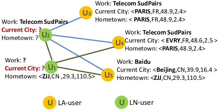
Figure 2 illustrates an example to show that the location sensitive attributes can be used to distinguish the weights among various LA-friends. Focusing on LN-user $u_{2}$ and his LA-friends $u_{3}$, $u_{4}$ and $u_{5}$, we notice that $u_{2}$ and $u_{3}$, $u_{4}$ work in the same institute, while $u_{5}$ works in another company which is far away from $u_{2}$’s workplace. In this case, it is natural to infer that $u_{2}$ is more likely to be living in the same city with $u_{3}$ and $u_{4}$ than with $u_{5}$; then $u_{3}$ and $u_{4}$ should be assigned with higher weights than $u_{5}$ because of the location similarity indicated by their workplace.

Inspired by the example, we construct an attribute-based location similarity matrix ($\mathcal{W}_{k}$) by each ($k$-th) location sensitive attribute ($a_{k}\in\mathcal{A}$). In the matrix, a cell $w_{k}^{ij}$ calculates the probability that two users live in the same city (i.e., location similarity) when they respectively have values of $a_{k_{i}}$ and $a_{k_{j}}$ regarding $a_{k}$. Specifically, we compute the total number of friend pairs where one user has a value of $a_{k_{i}}$ and the other has a value of $a_{k_{j}}$, denoted as $|\{a_{k}(u)=a_{k_{i}}\wedge a_{k}(v)=a_{k_{j}}\}|$; Among these friend pairs, we further count the pairs of friends who live in the same city, denoted as $|\{l(u)=l(v)\wedge a_{k}(u)=a_{k_{i}}\wedge a_{k}(v)=a_{k_{j}}\}|$. Then,

where $M$ is the number of possible values of attribute $a_{k}$ including $null$.

For a certain attribute $a_{k}$, assume that $u$ and his LA-friend $v$ have a value of $a_{k_{i}}$ and $a_{k_{j}}$ respectively. Then, the $u$ and $v$’s location similarity on $a_{k}$ can be easily obtained by indexing the $i$-th row and $j$-th column of $\mathcal{W}_{k}$, denoted as $w_{k}(u,v)=w_{k}^{ij},v\in\mathcal{F}^{{}^{LA}}(u)$.

We combine multiple location similarities on all the location sensitive attributes (e.g., work, hometown) with a set of trained parameters ($\mathbf{\beta}$) to measure $v$’s weight. This combined weight describes the probability that $u$ and $v$ live in the same city concerning all of their location sensitive attributes.

Then, LA-FLI model calculates the probability of $u$ living in $l_{i}$ by integrating all the weights of $u$’s LA-friends who live in $l_{i}$:

where $p_{{}_{LA-U}}(v,l_{i})$ represents whether or not the LA-friend $v$ living in $l_{i}$. It equals $1$ if $v$ states his current city is $l_{i}$; otherwise, it is $0$:

Before introducing LN-FLI model, we inspect the potential benefit of a user’s LN-friends for his current city prediction with another example shown in Figure 2. We observe that $u_{2}$, being a LN-friend of $u_{1}$, does not expose his current city; whereas, the workplace of $u_{2}$, Telecom SudParis, indicates two cities — Paris and Evry — according to the current cities of the users $u_{3}$ and $u_{4}$ who are also the employees of Telecom SudParis. Thereby, a user’s LN-friends can also reveal some location indications in their exposed attributes, which may help the prediction.

Therefore, for a LN-friend $v$, we first rely on his exposed location sensitive attributes and use PLI model (Sec. 5.1) to predict his current city, as:

Treating all the LN-friends equally, LN-FLI model integrates LN-friends’ location indications and computes the probability that $u$ lives in $l_{i}\in\mathcal{L}$ as:

Finally, primarily relying on LA-FLI model and being adjusted by LN-FLI model with a small regulator parameter $\lambda$, FLI model estimates the probability that $u$ currently lives in $l_{i}$ as:

We crawled Facebook by a Breadth First Search (BFS) [14] approach from March to June in $2012$ and collected $371,913$ users’ information including profile (e.g., gender, current city, hometown) and friends. Among all these users, $153,909$ users publicly report their current city (LA-users) and $225,314$ users do not reveal their current city (LN-users). All these users generate $12,863$ different locations. For more details about this data set, please refer to our previous work [17].

To evaluate the prediction approach, a user’s latest work or education experience is extracted as a location sensitive attribute, named ‘Work and Education’; we also exploit a user’s ‘Hometown’ as another location sensitive attribute. In our data set, $122,899$ LA-users show ‘Hometown’, $54,097$ LA-users reveal ‘Work and Education’ and $115,807$ LA-users publish their friend lists.

In addition to the exploited location sensitive information, some other information (e.g., a user’s geo-tagged posts) in Facebook may also leak the location. Our prediction approach can be extended to consider other location sensitive information smoothly, which we will discuss more in Sec. 9.1.

We first compare the different location selection approaches introduced in Sec. 6.3 to finalize the prediction approach with a good location selector. We also evaluate the performance of non-cluster prediction approach to show the effectiveness of location cluster. Specifically, these approaches can be denoted as:

• 1.

  $\textit{PFLI}_{prob}$ is a cluster based approach which selects the point of highest probability from the selected cluster as the predicted location.

• 2.

  $\textit{PFLI}_{cent}$ is a cluster based approach which selects the geographic centroid¹¹ 1 Geographic centroid is the average coordinate for all the points in a cluster while the probability of each point is considered as its weight. from the selected cluster as the predicted location.

• 3.

  $\textit{PFLI}_{dist}$ is a cluster based approach which selects the center of minimum distance from the selected cluster as the predicted location.

• 4.

  $\textit{PFLI}_{noclst}$ is a non-cluster approach which selects the point of highest probability from all candidate locations as the predicted location.

The proposed approaches are also compared to several state-of-the-art methods:

• 1.

  $\textit{Base}_{dist}$ predicts a user’s location based on the observation that the distance between two users decreases by the increase of their friendship [3].

• 2.

  $\textit{Base}_{ann}$ maps any location sensitive attribute value to a certain location and applies artificial neural network to train a current city prediction model [6].

• 3.

  $\textit{Base}_{freq}$, borrowing the idea from the prior works based on the Twitter data set [5][8], counts the frequency of locations that emerge in a user’s friends and predicts his current city by the most frequent location.

• 4.

  $\textit{Base}_{freq+}$ improves $\textit{Base}_{freq}$ by further using the neighborhood smoothing approach [8]. Given a location $l$, the points that are less than $20km$ apart from $l$ are considered as $l$’s neighborhoods.

• 5.

  $\textit{Base}_{knn}$ also relies on the frequency idea for Twitter; however, it merely counts on a user’s $k$ closest friends who have the most common friends with him to compute the most frequent location [1][2].

Among the above approaches, $\textit{Base}_{dist}$ and $\textit{Base}_{ann}$ are originally devised for Facebook; while $\textit{Base}_{freq}$, $\textit{Base}_{freq+}$ and $\textit{Base}_{knn}$ are on Twitter. We utilize the main ideas from $\textit{Base}_{freq}$, $\textit{Base}_{freq+}$ and $\textit{Base}_{knn}$, and adopt them to fit our data set. By comparing our approach to $\textit{Base}_{dist}$, $\textit{Base}_{freq}$, $\textit{Base}_{freq+}$ and $\textit{Base}_{knn}$ which mainly depend on friendships, we test the effectiveness of integrating location sensitive attributes. By comparing to $\textit{Base}_{ann}$, we examine the newly introduced one-attribute/multiple-locations mapping method.

Two widely used measurements: Average Error Distance (AED) and Accuracy within K km (ACC@K) [5][8][24] are exploited.

Error Distance computes the distance in kilometers between a user $u$’s real location and predicted location, i.e., $ErrDist(u)$. AED averages the Error Distances of the overall evaluated users, denoted as $\textit{AED}=\frac{\sum_{u\in U}ErrDist(u)}{|U|}$. In addition, we rank the users by their Error Distance in descending order and report AED of the top $60\%$, $80\%$ and $100\%$ of the evaluated users in the ranked list, denoted as $\textit{AED@}60\%$, $\textit{AED@}80\%$ and $\textit{AED@}100\%$ respectively [24].

Given a predefined Error Distance $K$ km, a prediction for a user is considered as a correct prediction, if the predicted Error Distance is less than $K$ km; otherwise, the prediction is incorrect. Then, Accuracy within K km is defined as the percentage of correct predictions (i.e., the percentage of users being predicted with an Error Distance less than $K$ km), denoted as $\textit{ACC@K}=\frac{|\{u|u\in U\wedge ErrDist(u)<K\}|}{|U|}$. ACC@K shows the prediction capability of an approach at a specific pre-established Error Distance.

Table 1 and Table 2 show the AEDs of all the compared approaches for two user sets. The smallest AEDs, which are generated by $\textit{PFLI}_{prob}$, have been highlighted in bold.

Let us first look at the PFLI model based approaches (i.e., $\textit{PFLI}_{dist}$, $\textit{PFLI}_{cent}$, $\textit{PFLI}_{prob}$, and $\textit{PFLI}_{noclst}$). Among the first three cluster based approaches that are different at their location selectors, $\textit{PFLI}_{dist}$ generates the largest AEDs while $\textit{PFLI}_{prob}$ achieves the smallest AEDs. We also compare the non-cluster approach $\textit{PFLI}_{noclst}$ and the cluster approach $\textit{PFLI}_{prob}$, which both select location of the highest probability. We observe that $\textit{PFLI}_{prob}$ presents smaller AEDs than $\textit{PFLI}_{noclst}$ and verify the effectiveness of the location cluster approach.

In addition, the results show that the PFLI model based approaches present much smaller AEDs than all the other baselines. In particular, the results demonstrate the PFLI model based approaches mapping one-attribute to multiple locations reduce the AED significantly compared to $\textit{Base}_{ann}$ which maps one-attribute to one-location.

By examining the results of AED@60%, AED@80% and AED@100%, we observe that the PFLI model based approaches can predict current city with relatively small AED@60% and AED@80%; whereas, AED@100% increases by $10$–$23$ times from AED@80%. This demonstrates the large Error Distance only occurs at predictions for a small number of users.

Lastly, we compare the results in the two Tables and notice that the prior approaches ($\textit{Base}_{dist}$, $\textit{Base}_{freq}$, $\textit{Base}_{freq+}$ and $\textit{Base}_{knn}$) predict locations with much larger AEDs for overall users than for users with LA-friends; however, for the PFLI model based approaches, AEDs differ slightly for two user sets. It demonstrates that a user’s profile can significantly contribute to the location prediction when the user’s friends’ locations are unavailable.

We study ACC@K of the three proposed prediction approaches ($\textit{PFLI}_{prob}$, $\textit{PFLI}_{cent}$ and $\textit{PFLI}_{dist}$) for two user sets in Figure 4. We observe that the accuracy of $\textit{PFLI}_{prob}$ goes up steadily with the increase of Error Distance. $\textit{PFLI}_{cent}$ may lead to very low accuracy when the pre-established Error Distance is quite small; but it can achieve higher accuracy than $\textit{PFLI}_{prob}$, when the pre-established Error Distance is larger than $40$ km. This reveals the properties of these two prediction approaches: $\textit{PFLI}_{cent}$, which selects the geographic centroid of a cluster, generates a short average Error Distance to all the locations in the cluster but fails to pick the user’s exact coordinate once it is not the centroid; while $\textit{PFLI}_{prob}$ may produce a large Error Distance if the location of the highest probability is not the user’s real location. In addition, $\textit{PFLI}_{dist}$ is not competitive with the other two approaches.

Rather than solely using any one of the proposed approaches, we exploit a combined-approach strategy by flexibly selecting the best approach according to the pre-established Error Distance. Specifically, this strategy uses $\textit{PFLI}_{prob}$ when the pre-established Error Distance is smaller than $40$ km and otherwise applies $\textit{PFLI}_{cent}$. The combination is practical and can obtain a better performance than using any single approach. We plot the combination line in Figure 4 and call it $\textit{PFLI}_{cmb}$.

Figure 5 compares $\textit{PFLI}_{cmb}$ to various baseline methods in terms of ACC@K. We observe that the proposed $\textit{PFLI}_{cmb}$ outperforms all the compared baselines for both user sets. Compared to $\textit{PFLI}_{noclst}$, $\textit{PFLI}_{cmb}$ increases around $1.5\%$ and $1.2\%$ of accuracy on average for users with LA-friends and overall users. This proves the effectiveness of the cluster strategy with successive cluster selection and location selection.

Comparing Figure 5(a) and 5(b), we observe that the approaches $\textit{Base}_{freq}$, $\textit{Base}_{freq+}$, $\textit{Base}_{dist}$ and $\textit{Base}_{knn}$ perform much worse for overall users than for users with LA-friends. This observation again indicates that these approaches depend heavily on the friends’ locations. However, in respect of the other approaches, which integrate location indications from both location sensitive attributes and friends (including our previous work $\textit{Base}_{ann}$ [6]), the prediction performance for overall users relatively approaches to the performance for users with LA-friends.

In the previous section, we observe that a user’s current city Exposure Probability is probably influenced by four factors: Error Distance, User Category, % Friends with Attributes and Cluster Confidence. Taking these four factors as features, we respectively use Random Decision Forest and Linear Regression approaches to model Exposure Probability. The performance of model is evaluated by two commonly used metrics, Mean Absolute Error (MAE) and Root Mean Squared Error (RMSE), with $10$-cross validation, shown in Table 5. We observe that the Random Decision Forest based model outperforms the Linear Regression based model by presenting smaller MAE and RMSE. Therefore, we employ the Random Decision Forest based model to estimate current city exposure probability, denoted as RDF Exposure Model.

Furthermore, ‘Leave-one-feature-out’ approach is exploited to verify the effectiveness of the features. We use Random Decision Forest approach to train exposure models by taking out any one of the four features, namely No Error Distance, No User Category, No % Friends with Attributes and No Cluster Confidence. Table 6 compares these ‘Leave-one-feature-out’ models to the RDF Exposure Model. We observe that the RDF Exposure Model presents the best performance with the smallest MAE and RMSE. The performance degradations when removing any one of the features just verify that all the four studied features contribute to the model. Cluster Confidence is observed as the most sensitive feature for the model, because the performance of the RDF Exposure Model drops most significantly when Cluster Confidence is taken out.

By exploiting the proposed current city exposure model, we construct an exposure estimator to forecast the exposure risk of a user’s private current city. Figure 9 illustrates the framework of the current city exposure estimator. The exposure estimator contains three main function modules: user information handler, current city exposure model and exposure risk level decision. The inputs of the exposure estimator include a user’s self-exposed information and a pre-established Error Distance. Given a user’s self-exposure information, the user information handler determines User Category, and computes Cluster Confidence and % Friends with Attributes. Based on the pre-established Error Distance, the obtained User Category, Cluster Confidence, and % Friends with Attributes, the exposure model calculates the current city exposure probability for the user. The exposure risk module determines a risk level according to the exposure probability. Finally, the exposure estimator outputs two risk measurements of current city: Exposure Probability and Risk Level.

References

- [1] Abrol, S., Khan, L., 2010. Tweethood: Agglomerative clustering on fuzzy k-closest friends with variable depth for location mining. In: SocialCom. pp. 153–160.
- [2] Abrol, S., Khan, L., Thuraisingham, B., 2012. Tweecalization: Efficient and intelligent location mining in twitter using semi-supervised learning. In: CollaborateCom. pp. 514–523.
- [3] Backstrom, L., Sun, E., Marlow, C., 2010. Find me if you can: Improving geographical prediction with social and spatial proximity. In: WWW. pp. 61–70.
- [4] Chakraborty, R., Vishik, C., Rao, H. R., 2013. Privacy preserving actions of older adults on social media: Exploring the behavior of opting out of information sharing. Decision Support Systems 55 (4), 948–956.
- [5] Chandra, S., Khan, L., Muhaya, F., 2011. Estimating twitter user location using social interactions–a content based approach. In: SocialCom. pp. 838–843.
- [6] Chanthaweethip, W., Han, X., Crespi, N., Chen, Y., Farahbakhsh, R., Cuevas, A., 2013. Current city prediction for coarse location based applications on facebook. In: GLOBECOM. pp. 3188–3193.
- [7] Chen, R., 2013. Living a private life in public social networks: An exploration of member self-disclosure. Decision Support Systems 55 (3), 661 – 668.
- [8] Cheng, Z., Caverlee, J., Lee, K., 2010. You are where you tweet: A content-based approach to geo-locating twitter users. In: CIKM. pp. 759–768.
- [9] Cranshaw, J., Toch, E., Hong, J., Kittur, A., Sadeh, N., 2010. Bridging the gap between physical location and online social networks. In: UbiComp. pp. 119–128.
- [10] Dey, R., Jelveh, Z., Ross, K., 2012a. Facebook users have become much more private: A large-scale study. In: PERCOM Workshop. pp. 346–352.
- [11] Dey, R., Tang, C., Ross, K., Saxena, N., 2012b. Estimating age privacy leakage in online social networks. In: INFOCOM. pp. 2836–2840.
- [12] Duckham, M., Kulik, L., 2006. Location privacy and location-aware computing. Dynamic & mobile GIS: investigating change in space and time 3, 35–51.
- [13] Farahbakhsh, R., Han, X., Cuevas, Á., Crespi, N., 2013. Analysis of publicly disclosed information in facebook profiles. In: ASONAM. pp. 699–705.
- [14] Gjoka, M., Kurant, M., Butts, C., Markopoulou, A., 2011. Practical recommendations on crawling online social networks. IEEE JSAC 29 (9), 1872–1892.
- [15] Gross, R., Acquisti, A., 2005. Information revelation and privacy in online social networks. In: WPES. pp. 71–80.
- [16] Han, X., ¨¢ngel Cuevas, Crespi, N., Cuevas, R., Huang, X., 2014. On exploiting social relationship and personal background for content discovery in {P2P} networks. Future Generation Computer Systems 40 (0), 17 – 29.
- [17] Han, X., Wang, L., Crespi, N., Park, S., Cuevas, Á., 2015. Alike people, alike interests? inferring interest similarity in online social networks. Decision Support Systems 69, 92–106.
- [18] Hastie, T., Tibshirani, R., Friedman, J., 2001. The Elements of Statistical Learning.
- [19] He, J., Chu, W. W., 2008. Protecting private information in online social networks. In: Intelligence and Security Informatics. pp. 249–273.
- [20] He, J., Chu, W. W., Liu, Z. V., 2006. Inferring privacy information from social networks. In: ISI. pp. 154–165.
- [21] Ikawa, Y., Vukovic, M., Rogstadius, J., Murakami, A., 2013. Location-based insights from the social web. In: WWW Companion. pp. 1013–1016.
- [22] Li, R., Wang, C., Chang, K. C.-C., 2014. User profiling in an ego network: co-profiling attributes and relationships. In: WWW. pp. 819–830.
- [23] Li, R., Wang, S., Chang, K. C.-C., 2012a. Multiple location profiling for users and relationships from social network and content. PVLDB 5 (11), 1603–1614.
- [24] Li, R., Wang, S., Deng, H., Wang, R., Chang, K. C.-C., 2012b. Towards social user profiling: Unified and discriminative influence model for inferring home locations. In: KDD. pp. 1023–1031.
- [25] Liben-Nowell, D., Novak, J., Kumar, R., Raghavan, P., Tomkins, A., 2005. Geographic routing in social networks. PNAS 102 (33), 11623–11628.
- [26] Lipford, H. R., Besmer, A., Watson, J., 2008. Understanding privacy settings in facebook with an audience view. UPSEC 8, 1–8.
- [27] Liu, Y., Krishnamurthy, B., Gummadi, K. P., 2011. Analyzing facebook privacy settings: User expectations vs. reality. In: IMC.
- [28] Mislove, A., Viswanath, B., Gummadi, K. P., Druschel, P., 2010. You are who you know: inferring user profiles in online social networks. In: WSDM. pp. 251–260.
- [29] Pontes, T., Magno, G., Vasconcelos, M., Gupta, A., Almeida, J., Kumaraguru, P., Almeida, V., 2012a. Beware of what you share: Inferring home location in social networks. In: ICDM Workshop. pp. 571–578.
- [30] Pontes, T., Vasconcelos, M., Almeida, J., Kumaraguru, P., Almeida, V., 2012b. We know where you live: privacy characterization of foursquare behavior. In: UbiComp. pp. 898–905.
- [31] Roth, M., Ben-David, A., Deutscher, D., Flysher, G., Horn, I., Leichtberg, A., Leiser, N., Matias, Y., Merom, R., 2010. Suggesting friends using the implicit social graph. In: KDD. pp. 233–242.
- [32] Ryoo, K., Moon, S., 2014. Inferring twitter user locations with 10 km accuracy. In: WWW Companion. pp. 643–648.
- [33] Schulz, A., Hadjakos, A., Paulheim, H., Nachtwey, J., Mühlhäuser, M., 2013. A multi-indicator approach for geolocalization of tweets. In: ICWSM.
- [34] Sokal, R. R., 1958. A statistical method for evaluating systematic relationships. Univ Kans Sci Bull 38, 1409–1438.
- [35] STELZNER, M. A., 2014. How marketers are using social media to grow their businesses.
- [36] Strater, K., Lipford, H. R., 2008. Strategies and struggles with privacy in an online social networking community. In: BCS-HCI. pp. 111–119.
- [37] Vicente, C. R., Freni, D., Bettini, C., Jensen, C. S., 2011. Location-related privacy in geo-social networks. IEEE Internet Computing 15 (3), 20–27.
- [38] Viswanath, B., Mislove, A., Cha, M., Gummadi, K. P., 2009. On the evolution of user interaction in facebook. In: Proceedings of the 2nd ACM workshop on Online social networks. pp. 37–42.
- [39] Xiang, R., Neville, J., Rogati, M., 2010. Modeling relationship strength in online social networks. In: WWW. pp. 981–990.
- [40] Zheleva, E., Getoor, L., 2009. To join or not to join: The illusion of privacy in social networks with mixed public and private user profiles. In: WWW. pp. 531–540.