A group theoretic approach to shear-free radiating stars

G. Abebe Email: gezahegn@aims.ac.za Affiliation: Astrophysics and Cosmology Research Unit, School of Mathematics, Statistics and Computer Science, University of KwaZulu–Natal, Private Bag X54001, Durban 4000, South Africa S. D. Maharaj Email: maharaj@ukzn.ac.za Affiliation: Astrophysics and Cosmology Research Unit, School of Mathematics, Statistics and Computer Science, University of KwaZulu–Natal, Private Bag X54001, Durban 4000, South Africa K. S Govinder Email: govinder@ukzn.ac.za Affiliation: Astrophysics and Cosmology Research Unit, School of Mathematics, Statistics and Computer Science, University of KwaZulu–Natal, Private Bag X54001, Durban 4000, South Africa

Abstract

A systematic analysis of the junction condition, relating the radial pressure with the heat flow in a shear-free relativistic radiating star, is undertaken. This is a highly nonlinear partial differential equation in general. We obtain the Lie point symmetries that leave the boundary condition invariant. Using a linear combination of the symmetries, we transform the junction condition into ordinary differential equations. We present several new exact solutions to the junction condition. In each case we can identify the exact solution with a Lie point generator. Some of the solutions obtained satisfy the linear barotropic equation of state. As a special case we regain conformally flat models which were found previously. Our analysis highlights the interplay between Lie algebras, nonlinear differential equations and application to relativistic astrophysics.

Keywords:

Lie symmetries; nonlinear equations; radiating stars

I Introduction

Radiating stars in a general relativistic context have been widely studied because of their importance in astrophysics. The detailed physics of such models have been investigated by Herrera et al. [1] with dissipation, by Di Prisco et al. [2] with charge, and Herrera et al. [3] with viscous dissipation in casual thermodynamics in the streaming and diffusion approximations. Particular models have been recently studied by Chan et al. [4] for an imperfect nonadiabatic distribution, by Pinheiro and Chan [5] with charge, and Pinheiro and Chan [6] for a collapsing body with an initial inhomogeneous density. Herrera and Santos [7] introduced the concept of Euclidean stars in general relativity by requiring that the areal radius and proper radius are equal. Exact models satisfying this condition were generated by Govender et al. [8] and Govinder and Govender [9]. Abebe et al. [10] showed that generalized Euclidean stars may be generated with an equation of state. An interesting feature of their approach is the application of Lie symmetries to produce models which are expanding, accelerating and shearing. This indicates that the Lie symmetry approach is helpful in solving the boundary junction condition, and highlights its role in astrophysical applications. We point out that in recent times Lie symmetry generators have been particularly useful in generating models in spherically symmetric gravitational fields. Msomi et al. [11, 12] have considered applications with heat flow and generated new classes of exact solutions. Kweyama et al. [13, 14] analysed Noether and Lie symmetries for charged relativistic fluids and were able to solve the field equations exactly.

The shear-free assumption in stellar models is often made in the study of relativistic radiating stars. Kolassis et al. [15] obtained the first exact solution with dissipation effects, satisfying the boundary conditions, for a shear-free radiating star in geodesic motion. Thirukkanesh and Maharaj [16] generated exact solutions for the geodesic model by transforming the junction condition into Bernoulli, Riccati, and confluent hypergeometric equations. This model was extended by Govender and Thirukkanesh [17] to include a nonzero cosmological constant. Note that in these treatments fluid particles travel along geodesics and the Friedmann dust solution in the absence of heat flow was regained in all cases. An important point here is that these treatments were performed under the condition of pressure isotropy and anisotropic pressures are absent. Ivanov [18] considered a general shear-free perfect fluid with heat flow that contains conformal flatness and geodesic models as a special case. A conformally flat relativistic model with dissipation and inhomogeneity was first proposed Herrera et al. [19]. This was integrated by Maharaj and Govender [20] and Herrera et al. [21] to obtained classes of exact solutions. Another class of conformally flat solutions was generated by Misthry et al. [22] by transforming the junction condition equation to an Abel equation. A further conformal flat radiating model, generated by a Lie symmetry was obtained by Abebe et al. [23]. Other models of shear-free radiating stars have been constructed by Tewari [24, 25], Pant et al. [26] and Pant and Tewari [27] which describe massive radiating fluid spheres and generated horizon-free collapse.

The shear-free assumption is utilised often in the analysis of self-gravitating spheres and when investigating gravitational collapse. This is largely due to the resulting simplification of the field equations. In addition, shear-free and the homogeneous expansion rate conditions are equivalent to the homology conditions in the Newtonian limit. Therefore the shear-free condition is well justified. However we need to make the observation that the shear-free condition may be unstable in the presence of anisotropic pressures and dissipative fluxes. The conditions under which an initially shear-free fluid continues to remain shear-free in its subsequent evolution has been studied by Herrera et al. [28]. In that analysis it was demonstrated that pressure anisotropy and dissipation affect the propagation of time and the gravitating relativistic fluid can become unstable.

We analyse a shear-free radiating model, without assuming conformal flatness and geodesic motion of fluid particles, in the presence of pressure anisotropy. We consider the Einstein field equations and boundary conditions in the context of Lie symmetries with the objective of producing new models of relativistic radiating objects. This is the main object of this paper. The case of shearing stellar models with Lie symmetries has been considered in some earlier treatments. Those treatments do not allow for vanishing shear and our results cannot be regained from such investigations. The absence of shear produces fundamentally a different set of field equations to be integrated. The Lie generators are generically different when the shear vanishes. In Sect. II we briefly discuss the shear-free radiating star and present the junction conditions. We show that the master equation is a nonlinear partial differential equation in the metric functions. In Sect. III we generate Lie symmetries for the master equation. Using the Lie point symmetries approach we transform the boundary condition to ordinary differential equations. By analyzing the resulting ordinary differential equations and transforming in the original variables we present new exact solutions in Sect. IV, V and VI. We link our solutions to specific Lie symmetry generators. In Sect. VII we show that some of our solutions satisfy a linear barotropic equation of state. We make concluding remarks, discuss the causal heat transport equation and summarize our solutions in tabular form in Sect. VIII.

II The model

We consider the particular case of spherically symmetric, shear-free radiating stellar models. The line element for the interior for the spacetimes is given by

ds^{2}=-A^{2}dt^{2}+B^{2}\left[dr^{2}+r^{2}\left(d\theta^{2}+\sin^{2}\theta d\phi^{2}\right)\right],

(1)

where $A$ and $B$ are metric functions of $t$ and $r$ . The acceleration and and expansion are nonzero but the fluid is shear-free.

The energy momentum tensor has the form

	$\displaystyle T_{ab}$	$\displaystyle=$	$\displaystyle\left(\mu+p_{\perp}\right)u_{a}u_{b}+p_{\perp}g_{ab}+(p_{\parallel}-p_{\perp})\chi_{a}\chi_{b}$		(2)
			$\displaystyle+q_{a}u_{b}+q_{b}u_{a},$		(2)

with heat flux and anisotropic stress. The fluid four-velocity $u^{a}=\frac{1}{A}\delta^{a}_{0}$ is comoving, $\chi^{a}$ is an unit four-vector along the radial direction $(u_{a}\chi^{a}=0)$ , and the heat flow vector $q^{a}=\left(0,q,0,0\right)$ is radially directed $(u_{a}q^{a}=0)$ . The Einstein field equations for the heat conducting spherically symmetric anisotropic fluid (2) become


$\displaystyle\mu$	$\displaystyle=$	$\displaystyle\frac{3}{A^{2}}\frac{B^{2}_{t}}{B^{2}}-\frac{1}{B^{2}}\left(2\frac{B_{rr}}{B}-\frac{B_{r}^{2}}{B^{2}}+\frac{4B_{r}}{rB}\right),$	(3a)
$\displaystyle p_{\parallel}$	$\displaystyle=$	$\displaystyle\frac{1}{A^{2}}\left(-2\frac{B_{tt}}{B}-\frac{B_{t}^{2}}{B^{2}}+2\frac{A_{t}}{A}\frac{B_{t}}{B}\right)$	(3b)
		$\displaystyle+\frac{1}{B^{2}}\left(\frac{B_{r}^{2}}{B^{2}}+2\frac{A_{r}}{A}\frac{B_{r}}{B}+\frac{2}{r}\frac{A_{r}}{A}+\frac{2}{r}\frac{B_{r}}{B}\right),$	(3b)
$\displaystyle p_{\perp}$	$\displaystyle=$	$\displaystyle-\frac{2}{A^{2}}\frac{B_{tt}}{B}+2\frac{A_{t}}{A^{3}}\frac{B_{t}}{B}-\frac{1}{A^{2}}\frac{B_{t}^{2}}{B^{2}}+\frac{1}{r}\frac{A_{r}}{A}\frac{1}{B^{2}}$	(3c)
		$\displaystyle+\frac{1}{r}\frac{B_{r}}{B^{3}}+\frac{A_{rr}}{A}\frac{1}{B^{2}}-\frac{B_{r}^{2}}{B^{4}}+\frac{B_{rr}}{B^{3}},$	(3c)
$\displaystyle q$	$\displaystyle=$	$\displaystyle-\frac{2}{AB^{2}}\left(-\frac{B_{rt}}{B}+\frac{B_{r}B_{t}}{B^{2}}+\frac{A_{r}}{A}\frac{B_{t}}{B}\right),$	(3d)

for the line element (1). The equations (3) describe the gravitational interactions in the interior of a shear-free spherically symmetric star with heat flux and anisotropic pressures.

The boundary of a radiating star divides the spacetime into interior and exterior regions. The interior spacetime (1) has to match across the boundary of the star to the Vaidya spacetime

	$\displaystyle ds^{2}$	$\displaystyle=$	$\displaystyle-\left(1-\frac{2m(v)}{R}\right)dv^{2}-2dvdR$		(4)
			$\displaystyle+R^{2}\left(d\theta^{2}+\sin^{2}\theta d\phi^{2}\right),$		(4)

which is the exterior. Here the quantity $m(v)$ denotes the mass of the star as measured by an observer at infinity. Matching leads to the junction conditions


$\displaystyle Adt$	$\displaystyle=$	$\displaystyle\left[\left(1-\frac{2m}{R_{\Sigma}}+2\frac{dR_{\Sigma}}{dv}\right)^{\frac{1}{2}}dv\right]_{\Sigma},$	(5a)
$\displaystyle\left(rB\right)_{\Sigma}$	$\displaystyle=$	$\displaystyle R_{\Sigma},$	(5b)
$\displaystyle m(v)$	$\displaystyle=$	$\displaystyle\left[\frac{r^{3}}{2}\left(\frac{BB_{t}^{2}}{A^{2}}-\frac{B_{r}^{2}}{B}\right)-r^{2}B_{r}\right]_{\Sigma},$	(5c)
$\displaystyle(p_{\parallel})_{\Sigma}$	$\displaystyle=$	$\displaystyle(Bq)_{\Sigma},$	(5d)

where the hypersurface $\Sigma$ defines the boundary of the radiating sphere. The particular junction condition (5d) should be solved, together with the field equations (3), to obtain the potentials $A$ and $B$ . This completes the model of a relativistic radiating star. The junction condition is a nonlinear differential equation

	$\displaystyle 2\frac{B_{rt}}{AB^{2}}+2\frac{B_{tt}}{A^{2}B}-2\frac{A_{t}B_{t}}{A^{3}B}-2\frac{B_{r}B_{t}}{AB^{3}}-2\frac{A_{r}B_{r}}{AB^{3}}$
	$\displaystyle-2\frac{A_{r}B_{t}}{A^{2}B^{2}}-\frac{B_{r}^{2}}{B^{4}}+\frac{B_{t}^{2}}{A^{2}B^{2}}-2\frac{A_{r}}{rAB^{2}}-2\frac{B_{r}}{rB^{3}}=0,$		(6)

valid at the boundary of shear-free radiating star. Equation (6) is the master equation that governs the evolution of the model.

III The master equation

We can use the Lie analysis of differential equations to find a solution to the master equation (6). In a general relativistic context, the Lie analysis has proved useful in cosmological settings as shown by Msomi et al. [11, 12], Kweyama et al. [13, 14] and Nyonyi et al. [29, 30], and in astrophysical applications as illustrated in the treatments by Abebe et al. [31, 10]. The general approach is described in these treatments and we will not repeat details here. Essentially we have to find infinitesimal Lie point generators that allow us to reduce a partial differential equation to ordinary differential equations. This is made possible by the existence of invariants associated with the Lie point symmetries of the partial differential equation equation (6).

The process has been adapted over time and is now algorithmic, and so can be implemented by different computer software packages. Utilizing the program PROGRAM LIE [32], we find that (6) admits the following Lie point symmetries:


$\displaystyle G_{1}$	$\displaystyle=$	$\displaystyle-Af^{\prime}(t)\frac{\partial}{\partial A}+f(t)\frac{\partial}{\partial t},$	(7a)
$\displaystyle G_{2}$	$\displaystyle=$	$\displaystyle A\frac{\partial}{\partial A}+B\frac{\partial}{\partial B},$	(7b)
$\displaystyle G_{3}$	$\displaystyle=$	$\displaystyle A\frac{\partial}{\partial A}+r\frac{\partial}{\partial r},$	(7c)

where $f(t)$ is an arbitrary function of $t$ . These symmetries generate invariants that can be used to reduce the partial differential equation (6) into ordinary differential equations for further analysis. Using the symmetries in (7) in turn, or taking any linear combination, may be helpful in reducing the master equation into ordinary differential equations. Since the symmetries do not have a nonzero Lie bracket relationship we do not consider the optimal system in this paper. As all combinations of these symmetries can be contained in a general linear combination, we take

	$\displaystyle aG_{1}+bG_{2}+cG_{3}$	$\displaystyle=$	$\displaystyle\left[c+b-af^{\prime}(t)\right]A\frac{\partial}{\partial A}+bB\frac{\partial}{\partial B}$		(8)
			$\displaystyle+af(t)\frac{\partial}{\partial t}+cr\frac{\partial}{\partial r},$		(8)

where $a$ , $b$ and $c$ are arbitrary constants. This combination gives the invariants


$\displaystyle x$	$\displaystyle=$	$\displaystyle\frac{\exp\left(\int^{t}\frac{dt}{af(t)}\right)}{r^{1/c}},$	(9a)
$\displaystyle A$	$\displaystyle=$	$\displaystyle\frac{h(x)}{f(t)}\exp\left(\int^{t}\frac{cdt}{af(t)}+\int^{t}\frac{bdt}{af(t)}\right),$	(9b)
$\displaystyle B$	$\displaystyle=$	$\displaystyle g(x)r^{b/c},$	(9c)

where $a\neq 0$ and $c\neq 0$ . The quantities $g(x)$ and $h(x)$ are arbitrary functions associated with the Lie symmetry generators and arise from integration.

Using the invariants (9) we can write (6) in the form

	$\displaystyle\left[2a^{2}gx^{2b+2c+1}\left((b+c)g-xg^{\prime}\right)\right]h^{\prime}h^{2}$
	$\displaystyle+2acx^{b+c+2}g^{2}g^{\prime}h^{\prime}h-2c^{2}x^{2}g^{3}g^{\prime}h^{\prime}$
	$\displaystyle+\left[c^{2}xg^{2}\left(xg^{\prime 2}-2g\left((b+c-1)g^{\prime}-xg^{\prime\prime}\right)\right)\right]h$
	$\displaystyle-\left[2acgx^{b+c+1}\left(g\left(xg^{\prime\prime}+g^{\prime}\right)-xg^{\prime 2}\right)\right]h^{2}$
	$\displaystyle+\left[a^{2}x^{2(b+c)}\left(xg^{\prime}-bg\right)\left((b+2c)g-xg^{\prime}\right)\right]h^{3}=0,$		(10)

where primes denote differentiation with respect to to the new variable $x$ . Note that the partial differential equation (6) has been reduced to the ordinary differential equation (10). Equation (10) is difficult to solve in general. To demonstrate an exact solution it is necessary to make assumptions on the parameters and arbitrary functions.

To progress we make the assumption

g(x)=kh(x).

(11)

Then equation (10) reduces to the form

	$\displaystyle 2ckx^{2}\left[ck-ax^{b+c}\right]hh^{\prime\prime}$
	$\displaystyle-x^{2}\left[3a^{2}x^{2(b+c)}-4ackx^{b+c}+c^{2}k^{2}\right]h^{\prime 2}$
	$\displaystyle-2x\left[c^{3}k^{2}-2a^{2}bx^{2(b+c)}-acx^{b+c}\left(2ax^{b+c}-k\right)\right.$
	$\displaystyle\left.+(b-1)c^{2}k^{2}\right]hh^{\prime}-a^{2}b[b+2c]x^{2(b+c)}h^{2}=0.$		(12)

Equation (12) is a nonlinear second order differential equation. We can reduce (12) to first order if we let

y=\frac{h^{\prime}}{h}.

(13)

Then the transformation (13) enables us to write (12) in the form

	$\displaystyle y^{\prime}+\left(\frac{3ax^{b+c}}{2ck}+\frac{1}{2}\right)y^{2}+\left[2a^{2}bx^{2(b+c)}+acx^{b+c}\right.$
	$\displaystyle\times\left.\left(2ax^{b+c}-k\right)+(1-b)c^{2}k^{2}-c^{3}k^{2}\right]$
	$\displaystyle\left[ckx\left(ck-ax^{b+c}\right)\right]^{-1}y+\frac{a^{2}b(b+2c)x^{2(b+c-1)}}{2ck\left(ax^{b+c}-ck\right)}=0.$

Observe that (III) is a Riccati equation in the variable $y$ . Riccati equations can be transformed to second order linear equations. We let

u(x)=\exp\left[\int^{x}\left(\frac{3ax^{b+c}}{2ck}+\frac{1}{2}\right)y(x)dx\right].

(15)

Note that in equation (15) the term $\left(\frac{3ax^{b+c}}{2ck}+\frac{1}{2}\right)$ is the coefficient of the quantity $y^{2}$ in (III). Using (15) equation (III) is transformed to

u^{\prime\prime}+\gamma(x)u^{\prime}+\zeta(x)u=0,\qquad

(16)

where


$\displaystyle\gamma(x)$	$\displaystyle=$	$\displaystyle\left[6a^{3}bx^{3(b+c)}+a^{2}cx^{2(b+c)}\left(6ax^{b+c}+(5b-3)k\right)\right.$
		$\displaystyle\left.-c^{3}k^{2}\left(6ax^{b+c}+(b-1)k\right)\right.$
		$\displaystyle\left.+ac^{2}kx^{b+c}\left(5ax^{b+c}+(2-6b)k\right)-c^{4}k^{3}\right]$
		$\displaystyle\times\left[ckx\left(-3a^{2}x^{2(b+c)}+2ackx^{b+c}+c^{2}k^{2}\right)\right]^{-1},$
$\displaystyle\zeta(x)$	$\displaystyle=$	$\displaystyle\frac{a^{2}b(b+2c)x^{2(b+c-1)}\left(3ax^{b+c}+ck\right)}{4c^{2}k^{2}\left(ax^{b+c}-ck\right)}.$	(17b)

Therefore we have the remarkable feature that the second order nonlinear equation (12) has been transformed to the linear equation (16) via the transformations (13) and (15).

Particular choices of the constants $a,b$ and $c$ allow us to integrate (10), (12) or (16) and obtain potentials for the gravitational field. There are several classes that arise which we consider in turn.

IV Class I

In this class we make the restrictions that $a\neq 0$ and $c\neq 0$ . These conditions arise so that the invariants (9) exist.

IV.1 Case I(a): $b=0$

If we set $b=0$ then the coefficient of the linear term in $u$ in (16) disappears. In this case we have

	$\displaystyle u^{\prime\prime}+\left[3a^{2}x^{2c}\left(2ax^{c}-k\right)+c^{2}k^{2}\left(k-6ax^{c}\right)\right.$
	$\displaystyle\left.+ackx^{c}\left(5ax^{c}+2k\right)-c^{3}k^{3}\right]\left[kx\left(-3a^{2}x^{2c}\right.\right.$
	$\displaystyle\left.\left.+2ackx^{c}+c^{2}k^{2}\right)\right]^{-1}u^{\prime}=0,$		(18)

which is a separable equation. This can be easily integrated to give

u(x)=d\exp\left(\frac{2ax^{c}}{ck}\right)\left(6a^{2}x^{2c}-10ackx^{c}+3c^{2}k^{2}\right)+\tilde{m},

(19)

where $d$ and $\tilde{m}$ are constants. Then equation (15) yields

y(x)=\frac{8acx^{c-1}\exp\left(\frac{2ax^{c}}{ck}\right)\left(ax^{c}-ck\right)}{\exp\left(\frac{2ax^{c}}{ck}\right)\left(6a^{2}x^{2c}+3c^{2}k^{2}-10ackx^{c}\right)+m},

(20)

where $m=\frac{\tilde{m}}{d}$ is a new constant.

Hence we obtain the potentials


$\displaystyle A$	$\displaystyle=$	$\displaystyle\frac{n}{f(t)}\exp\left(\int^{x}\left[8acx^{c-1}\exp\left(\frac{2ax^{c}}{ck}\right)\left(ax^{c}-ck\right)\right]\right.$	(21a)
		$\displaystyle\times\left.\left[\exp\left(\frac{2ax^{c}}{ck}\right)\left(6a^{2}x^{2c}-10ackx^{c}\right.\right.\right.$
		$\displaystyle\left.\left.\left.+3c^{2}k^{2}\right)+m\right]^{-1}\,dx+\int^{t}\frac{cdt}{af(t)}\right),$
$\displaystyle B$	$\displaystyle=$	$\displaystyle\frac{kf(t)}{\exp\left(\int^{t}\frac{cdt}{af(t)}\right)}A,$	(21b)

where $x=\exp\left(\int^{t}\frac{\,dt}{af(t)}\right)r^{-1/c}$ and $n$ is an arbitrary constant of integration. We believe that this solution is not contained in the literature.

It is possible to evaluate the integral containing $x$ in (21a) when $m=0$ . In this case

$\displaystyle A$	$\displaystyle=$	$\displaystyle\tilde{n}\left(6a^{2}x^{2c}-10ackx^{c}+3c^{2}k^{2}\right)^{2/3}$	(22)
		$\displaystyle\times\frac{\exp\left(\int^{t}\frac{cdt}{af(t)}\right)}{f(t)}\left(\frac{7-\frac{3\sqrt{7}ckx^{-c}}{a}+5\sqrt{7}}{\frac{3\sqrt{7}ckx^{-c}}{a}-5\sqrt{7}+7}\right)^{\frac{4}{\sqrt{7}}}$
		$\displaystyle\times\left(\frac{7-\frac{6\sqrt{7}ax^{c}}{ck}+5\sqrt{7}}{\frac{6\sqrt{7}ax^{c}}{ck}-5\sqrt{7}+7}\right)^{\frac{10}{3\sqrt{7}}},$

and $\tilde{n}$ is a new constant. For this special case the explicit dependence on the variable $x$ is fully specified; there is freedom only in the variable $t$ .

IV.2 Case I(b): $b=-c$

If we set $b=-c$ then equation (16) becomes

x^{2}u^{\prime\prime}+xu^{\prime}+\frac{a^{2}(3a+ck)}{4k^{2}(ck-a)}u=0,

(23)

which is a simpler form. It is interesting to note that this case produces the Euler equation (23). We can integrate (23) to obtain

	$\displaystyle u(x)$	$\displaystyle=$	$\displaystyle\tilde{c_{1}}\cosh\left(\frac{a\sqrt{3a+ck}}{2k\sqrt{a-ck}}\log(x)\right)$		(24)
			$\displaystyle+\tilde{c_{2}}\sinh\left(\frac{a\sqrt{3a+ck}}{2k\sqrt{a-ck}}\log(x)\right),$		(24)

where $\tilde{c_{1}}$ and $\tilde{c_{2}}$ are arbitrary constants of integration. Then from (15) we obtain

y(x)=\frac{ac\sqrt{3a+ck}}{\sqrt{a-ck}}\frac{c_{1}x^{\frac{a\sqrt{3a+ck}}{k\sqrt{a-ck}}}-c_{2}}{x\left(3ax^{c}+ck\right)\left(c_{1}x^{\frac{a\sqrt{3a+ck}}{k\sqrt{a-ck}}}+c_{2}\right)},

(25)

where $c_{1}=\tilde{c_{1}}+\tilde{c_{2}}$ and $c_{2}=\tilde{c_{1}}-\tilde{c_{2}}$ .

Hence we have the potentials


$\displaystyle A$	$\displaystyle=$	$\displaystyle\frac{1}{f(t)}\left(m\left[r^{-1/c}\exp\left(\int^{t}\frac{dt}{af(t)}\right)\right]^{\frac{a\sqrt{3a+ck}}{2k\sqrt{a-ck}}}\right.$
		$\displaystyle\left.+n\left[r^{-1/c}\exp\left(\int^{t}\frac{dt}{af(t)}\right)\right]^{-\frac{a\sqrt{3a+ck}}{2k\sqrt{a-ck}}}\right){}^{\frac{2ck}{3a+ck}},$
$\displaystyle B$	$\displaystyle=$	$\displaystyle k\frac{f(t)}{r}A,$	(26b)

where $m=c_{1}c_{3}^{\frac{3a+ck}{2ck}}$ and $n=c_{2}c_{3}^{\frac{3a+ck}{2ck}}$ are constants. This is another new solution to the master equation.

IV.3 Subclass I(c): $b=-c$ , $k=-3a/c$

Note that in (26), $k\neq-3a/c$ . With the values $b=-c$ and $k=-3a/c$ the transformation (15) leads to an inconsistency. This means that we have to integrate (12) or (III) for this case. If we set $k=-3a/c$ and $b=-c$ , then equation (12) becomes

24x^{2}hh^{\prime\prime}-24x^{2}h^{\prime 2}+24xhh^{\prime}+c^{2}h^{2}=0,

(27)

which is greatly simplified. Now (27) can be integrated to give

h(x)=\frac{nx^{m}}{\exp\left[\frac{c^{2}}{48}\log^{2}(x)\right]},

(28)

where $m$ and $n$ are constants of integration.

Hence we get the metric functions


$\displaystyle A$	$\displaystyle=$	$\displaystyle\frac{n}{f(t)}\frac{\left[r^{-1/c}\exp\left(\int^{t}\frac{dt}{af(t)}\right)\right]^{m}}{\exp\left(\frac{c^{2}}{48}\log^{2}\left[r^{-1/c}\exp\left(\int^{t}\frac{dt}{af(t)}\right)\right]\right)},$	(29a)
$\displaystyle B$	$\displaystyle=$	$\displaystyle-\frac{3a}{c}\frac{f(t)}{r}A.$	(29b)

This is also another new solution to the master equation (6).

IV.4 Case I(d): $b=-2c$

If we set $b=-2c$ then the coefficient of the linear term in $u$ in (16) disappears as in Case I(a). Then we obtain

	$\displaystyle u^{\prime\prime}-\left[\left(x^{-c-1}\left(6a^{3}+a^{2}(5c+3)kx^{c}-2ac(3c+1)k^{2}x^{2c}\right.\right.\right.$
	$\displaystyle\left.\left.\left.-c^{2}(c+1)k^{3}x^{3c}\right)\right)\right]\left[k\left(3a^{2}-2ackx^{c}\right.\right.$
	$\displaystyle\left.\left.-c^{2}k^{2}x^{2c}\right)\right]^{-1}u^{\prime}=0,$		(30)

which is separable. This can be easily integrated to give

	$\displaystyle u(x)$	$\displaystyle=$	$\displaystyle dk\exp\left(\frac{2ax^{-c}}{ck}\right)\left(\frac{3c^{2}k^{2}}{a}+6ax^{-2c}\right.$		(31)
			$\displaystyle\left.-10ckx^{-c}\right)+\tilde{m},$		(31)

where the constants $d$ and $\tilde{m}$ result from the integration. Then equation (15) yields

$\displaystyle y(x)$	$\displaystyle=$	$\displaystyle\left[8ac\exp\left(\frac{2ax^{-c}}{ck}\right)\left(ckx^{c}-a\right)\right]$	(32)
		$\displaystyle\times\left[x\left(\exp\left(\frac{2ax^{-c}}{ck}\right)\left[6a^{2}+3c^{2}k^{2}x^{2c}\right.\right.\right.$
		$\displaystyle\left.\left.\left.-10ackx^{c}\right]+mx^{2c}\right)\right]^{-1},$

where $m=\frac{\tilde{m}}{d}$ is a constant.

Hence we can generate the potentials


$\displaystyle A$	$\displaystyle=$	$\displaystyle\frac{n}{f(t)}\exp\left(\int^{x}\left[8ac\exp\left(\frac{2ax^{-c}}{ck}\right)\left(ckx^{c}-a\right)\right]\right.$	(33a)
		$\displaystyle\left.\times\left[x\left(\exp\left(\frac{2ax^{-c}}{ck}\right)\left[6a^{2}+3c^{2}k^{2}x^{2c}-10ackx^{c}\right]\right.\right.\right.$
		$\displaystyle\left.\left.\left.+mx^{2c}\right)\right]^{-1}\,dx-\int^{t}\frac{cdt}{af(t)}\right),$
$\displaystyle B$	$\displaystyle=$	$\displaystyle\frac{kf(t)}{\exp\left(\int^{t}\frac{cdt}{af(t)}\right)}A,$	(33b)

where $x=\exp\left(\int^{t}\frac{\,dt}{af(t)}\right)r^{-1/c}$ and $n$ is new arbitrary constant. This is a new model.

This class of solution contains a previously found model. To show this we set

a=c=k=1\text{ and }f(t)=t.

(34)

Then solution (33) becomes

	$\displaystyle A$	$\displaystyle=$	$\displaystyle B$
		$\displaystyle=$	$\displaystyle d\exp\left(\int_{1}^{t/r}\frac{8\exp\left(2z\right)(z-1)}{\exp\left(2z\right)\left(6z^{2}-10z+3\right)+m}\,dz\right),$

which is a self-similar solution for the master equation. It has been obtained previously by Abebe et al. [23] when analyzing a conformally flat radiating star.

V Class II

In this class we set $a=0$ . Then the invariants (9) do not exist. For this category of solution we then have to consider the symmetry

bG_{2}+cG_{3}=\left(c+b\right)A\frac{\partial}{\partial A}+bB\frac{\partial}{\partial B}+cr\frac{\partial}{\partial r},

(36)

from (8). The invariants associated with (36) are


$\displaystyle A$	$\displaystyle=$	$\displaystyle h(t)r^{(b+c)/c},$	(37a)
$\displaystyle B$	$\displaystyle=$	$\displaystyle g(t)r^{b/c},\text{ and }$	(37b)
$\displaystyle t.$			(37c)

The invariants (37) reduce the master equation (6) to

	$\displaystyle 2c^{2}gg^{\prime}h^{\prime}-c^{2}\left(2gg^{\prime\prime}+g^{\prime 2}\right)h+2c(b+c)g^{\prime}h^{2}$
	$\displaystyle+\left(3b^{2}+6bc+2c^{2}\right)h^{3}=0.$		(38)

Here the primes stand for the derivatives with respect to the independent variable $t$ . Equation (38) is an Abel differential equation in $h$ . It is not possible to integrate it in general. Particular solutions do exist as we now demonstrate. We set

b=\left(\pm\frac{\sqrt{3}}{3}-1\right)c,

(39)

to simplify the Abel equation. Then (38) becomes

6gg^{\prime}h^{\prime}-3\left(2gg^{\prime\prime}+g^{\prime 2}\right)h\pm 2\sqrt{3}g^{\prime}h^{2}=0.

(40)

The advantage of (40) is that it is a Bernoulli equation in $h$ . It is interesting to note that it can be integrated even when the function $g$ is unspecified. We integrate (40) to obtain

h(t)=\pm\frac{\sqrt{3}}{2}\frac{g^{\prime}\sqrt{g}}{\sqrt{g}+d},

(41)

where $d$ is a constant of integration.

Hence the potentials functions become


$\displaystyle A$	$\displaystyle=$	$\displaystyle\pm\frac{\sqrt{3}}{2}\frac{g^{\prime}\sqrt{g}}{\sqrt{g}+d}r^{\pm\frac{\sqrt{3}}{3}},$	(42a)
$\displaystyle B$	$\displaystyle=$	$\displaystyle gr^{\pm\frac{\sqrt{3}}{3}-1},$	(42b)

which is a new exact solution for the shear-free model.

Other exact solutions to (38) exist but they may not be realistic. For example, (38) can be integrated to yield exact solutions if we assume $c=-b$ and $g(t)=kh(t)$ . Unfortunately the model then become unphysical as the heat flux vanishes when $g(t)=kh(t)$ and both the tangential pressure and the energy density vanish when $c=-b$ .

VI Class III

In this class we set $c=0$ . Consequently the invariants (9) are not defined. Therefore in this case we consider the symmetry

aG_{1}+bG_{2}=(b-af^{\prime}(t))A\frac{\partial}{\partial A}+B\frac{\partial}{\partial B}+af(t)\frac{\partial}{\partial t},

(43)

from (8). Note that the invariants arising from (43) are given by


$\displaystyle A$	$\displaystyle=$	$\displaystyle h(r)\frac{\exp\left(\int\frac{bdt}{af(t)}\right)}{f(t)},$	(44a)
$\displaystyle B$	$\displaystyle=$	$\displaystyle g(r)\exp\left(\int\frac{bdt}{af(t)}\right),\text{ and }$	(44b)
$\displaystyle r.$			(44c)

Using the invariants (44) the master equation (6) is reduced to give

	$\displaystyle 2a^{2}g\left(rg^{\prime}+g\right)hh^{\prime}+2abrg^{3}h^{\prime}+a^{2}g^{\prime}\left(rg^{\prime}+2g\right)h^{2}$
	$\displaystyle-b^{2}rg^{4}=0,$		(45)

where the primes denote derivatives with respect to the independent variable $r$ . Equation (45) is highly nonlinear and cannot be easily integrated in general. We assume that

g(r)=kh(r),

(46)

so that (45) becomes

\left(\frac{h^{\prime}}{h}\right)^{2}+\frac{2}{3}\left(\frac{bk}{a}+\frac{2}{r}\right)\frac{h^{\prime}}{h}-\frac{b^{2}k^{2}}{3a^{2}}=0.

(47)

We observe that (47) may be treated as a quadratic equation in the quantity $\frac{h^{\prime}}{h}$ ; this gives

\frac{h^{\prime}}{h}=\frac{\pm 2\sqrt{a^{2}\left(a^{2}+abkr+b^{2}k^{2}r^{2}\right)}-2a^{2}-abkr}{3a^{2}r}.

(48)

The two roots in (48) can be integrated to yield two different classes of solutions


$\displaystyle h(r)$	$\displaystyle=$	$\displaystyle\frac{d}{r^{4/3}}\left(\frac{\left(\alpha(r)+2a^{2}+abkr\right)^{2}}{\left(\alpha(r)+2abkr+a^{2}\right)}\right)^{1/3}$	(49a)
		$\displaystyle\times\exp\left(\frac{-\alpha(r)-abkr}{3a^{2}}\right),$	(49a)
$\displaystyle h(r)$	$\displaystyle=$	$\displaystyle d\left(\frac{\alpha(r)+2abkr+a^{2}}{\left(\alpha(r)+2a^{2}+abkr\right)^{2}}\right)^{1/3}$	(49b)
		$\displaystyle\times\exp\left(\frac{\alpha(r)-abkr}{3a^{2}}\right),$	(49b)

where $\alpha(r)=2a\sqrt{a^{2}+abkr+b^{2}k^{2}r^{2}}$ and $d$ is an arbitrary constant of integration.

Hence we have


$\displaystyle A$	$\displaystyle=$	$\displaystyle\frac{d}{r^{4/3}f(t)}\left(\frac{\left(\alpha(r)+2a^{2}+abkr\right)^{2}}{\left(\alpha(r)+2abkr+a^{2}\right)}\right)^{1/3}$	(50a)
		$\displaystyle\times\exp\left(\int\frac{bdt}{af(t)}-\frac{\alpha(r)}{3a^{2}}-\frac{bkr}{3a}\right),$	(50a)
$\displaystyle B$	$\displaystyle=$	$\displaystyle kf(t)A,$	(50b)

and


$\displaystyle A$	$\displaystyle=$	$\displaystyle\frac{d}{f(t)}\left(\frac{\alpha(r)+2abkr+a^{2}}{\left(\alpha(r)+2a^{2}+abkr\right)^{2}}\right)^{1/3}$	(51a)
		$\displaystyle\times\exp\left(\int\frac{bdt}{af(t)}+\frac{\alpha(r)}{3a^{2}}-\frac{bkr}{3a}\right),$	(51a)
$\displaystyle B$	$\displaystyle=$	$\displaystyle kf(t)A,$	(51b)

which are two classes of solution to the master equation.

This category of solutions reduces to known models. We can show this by setting

f(t)=1\text{ and }b=d=k=1.

(52)

Then the solutions (50) and (51) become


$\displaystyle A$	$\displaystyle=$	$\displaystyle B$	(53a)
	$\displaystyle=$	$\displaystyle r^{-4/3}\exp\left(\frac{t}{a}-\frac{\alpha(r)}{3a}-\frac{r}{3a}\right)$
		$\displaystyle\times\left(\frac{\left(\alpha(r)+2a+r\right)^{2}}{\left(\alpha(r)+a+2r\right)}\right)^{1/3},$
$\displaystyle A$	$\displaystyle=$	$\displaystyle B$	(53b)
	$\displaystyle=$	$\displaystyle\exp\left(\frac{t}{a}-\frac{r}{3a}+\frac{\alpha(r)}{3a}\right)$
		$\displaystyle\times\left(\frac{\alpha(r)+a+2r}{\left(\alpha(r)+2a+r\right)^{2}}\right)^{1/3},$

respectively. These solutions were previously obtained by Abebe et al. [23] for a radiating star which has the property of conformal flatness.

VII Equations of state

In relativistic astrophysics it is important that the model should admit an equation of state on physical grounds. Many exact solutions for a radiating star that have been found before do not satisfy this condition. We can report that particular classes of models in this paper do admit a linear equation of state which are barotropic. We give each of these cases below and associate them with the relevant Lie symmetry.

(a) The generator $aG_{1}-cG_{2}+cG_{3}$ $(k\neq-\frac{3a}{c})$

Using the generator $aG_{1}-cG_{2}+cG_{3}$ we can obtain a model from (26) which admits an equation of state. The line element for this case is

	$\displaystyle ds^{2}$	$\displaystyle=$	$\displaystyle\left[\left(m\psi^{1/2}+n\psi^{-1/2}\right){}^{\frac{2ck}{3a+ck}}\right]^{2}\left(-\left[\frac{1}{f(t)}\right]^{2}dt^{2}\right.$		(54)
			$\displaystyle\left.+\left[\frac{k}{r}\right]^{2}\left[dr^{2}+r^{2}\left(d\theta^{2}+\sin^{2}\theta d\phi^{2}\right)\right]\right),$		(54)

where $\psi=\left[r^{-1/c}\exp\left(\int\frac{\,dt}{af(t)}\right)\right]^{\frac{a\sqrt{3a+ck}}{k\sqrt{a-ck}}}$ . The matter variables become


$\displaystyle\mu$	$\displaystyle=$	$\displaystyle\left[2\left(a^{2}-ack+c^{2}k^{2}\right)\left(ck\left(m^{2}\psi^{2}-4mn\psi+n^{2}\right)\right.\right.$	(55a)
		$\displaystyle\left.\left.-6amn\psi\right)\right]\left[ck^{3}(a-ck)(3a+ck)\left(m\psi+n\right)^{2}\right.$
		$\displaystyle\left.\times\left(\psi^{-1/2}\left(m\psi+n\right)\right)^{\frac{4ck}{3a+ck}}\right]^{-1},$
$\displaystyle p_{\parallel}$	$\displaystyle=$	$\displaystyle\left[2a\left(6amn\psi-ck\left(m^{2}\psi^{2}-4mn\psi+n^{2}\right)\right)\right]$	(55b)
		$\displaystyle\times\left[k^{2}(ck-a)(3a+ck)\left(m\psi+n\right)^{2}\right.$
		$\displaystyle\left.\times\left(\psi^{-1/2}\left(m\psi+n\right)\right)^{\frac{4ck}{3a+ck}}\right]^{-1},$
$\displaystyle p_{\perp}$	$\displaystyle=$	$\displaystyle\left[(a+ck)\left(\psi^{-1/2}\left(m\psi+n\right)\right)^{-\frac{4ck}{3a+ck}}\left(12amn\psi\right.\right.$	(55c)
		$\displaystyle\left.\left.+ck\left(m\psi+n\right)^{2}\right)\right]\left[ck^{3}(3a+ck)\left(m\psi+n\right)^{2}\right.$
		$\displaystyle\left.\times\left(\psi^{-1/2}\left(m\psi+n\right)\right)^{\frac{4ck}{3a+ck}}\right]^{-1},$
$\displaystyle q$	$\displaystyle=$	$\displaystyle\left[\frac{k}{r}\left(m\psi^{1/2}+n\psi^{-1/2}\right){}^{\frac{2ck}{3a+ck}}\right]^{-1}p_{\parallel}.$	(55d)

From the above we generate the linear barotropic equation of state

p_{\parallel}=\lambda\mu,\quad\lambda=\frac{ack}{a^{2}-ack+c^{2}k^{2}},

(56)

provided that $k\neq-\frac{3a}{c}$ .

(b) The generator $aG_{1}-cG_{2}+cG_{3}$ $(k=-\frac{3a}{c})$

The generator $aG_{1}-cG_{2}+cG_{3}$ helps to find another model (29) when $k=-\frac{3a}{c}$ . This model also admits an equation of state. The line element for this case is given by

	$\displaystyle ds^{2}$	$\displaystyle=$	$\displaystyle\left[\frac{n\varphi^{m}}{\exp\left(\frac{c^{2}}{48}\log^{2}\varphi\right)}\right]^{2}\left[-\left(1/f(t)\right)^{2}dt^{2}+9\left(a/(cr)\right)^{2}\right.$		(57)
			$\displaystyle\left.\times\left[dr^{2}+r^{2}\left(d\theta^{2}+\sin^{2}\theta d\phi^{2}\right)\right]\right],$		(57)

where $\varphi=r^{-1/c}\exp\left(\int\frac{dt}{af(t)}\right)$ . The matter variables become


$\displaystyle\mu$	$\displaystyle=$	$\displaystyle\left[13\left(c^{4}\log^{2}\varphi-48mc^{2}\log\varphi+24\left(c^{2}+24m^{2}\right)\right)\right.$	(58a)
		$\displaystyle\left.\times\exp\left(\frac{1}{24}c^{2}\log^{2}\varphi\right)\right]\left[2592a^{2}n^{2}\varphi^{2m}\right]^{-1},$	(58a)
$\displaystyle p_{\parallel}$	$\displaystyle=$	$\displaystyle\left[\left(48mc^{2}\log\varphi-c^{4}\log^{2}\varphi-24\left(c^{2}+24m^{2}\right)\right)\right.$	(58b)
		$\displaystyle\left.\times\exp\left(\frac{1}{24}c^{2}\log^{2}\varphi\right)\right]\left[864a^{2}n^{2}\varphi^{2m}\right]^{-1},$	(58b)
$\displaystyle p_{\perp}$	$\displaystyle=$	$\displaystyle\left[\left(48mc^{2}\log\varphi-c^{4}\log^{2}\varphi+48c^{2}+576m^{2}\right)\right.$	(58c)
		$\displaystyle\left.\times\exp\left(\frac{1}{24}c^{2}\log^{2}\varphi\right)\right]\left[648a^{2}n^{2}\varphi^{2m}\right]^{-1},$	(58c)
$\displaystyle q$	$\displaystyle=$	$\displaystyle\left[\frac{3a}{cr}\frac{n\varphi^{m}}{\exp\left(\frac{c^{2}}{48}\log^{2}\varphi\right)}\right]^{-1}p_{\parallel}.$	(58d)

We observe that this case also admits an equation of state

p_{\parallel}=\lambda\mu,\quad\lambda=-\frac{3}{13},

(59)

which is linear and barotropic.

(c) The generator $bG_{2}+cG_{3}$

The generator $bG_{2}+cG_{3}$ can also associated with an equation of state. The line element for this model becomes

	$\displaystyle ds^{2}$	$\displaystyle=$	$\displaystyle-\frac{3}{4}g^{\prime 2}r^{\pm 2\frac{\sqrt{3}}{3}}dt^{2}+g^{2}r^{\pm\frac{2\sqrt{3}}{3}-2}\left[dr^{2}\right.$		(60)
			$\displaystyle\left.+r^{2}\left(d\theta^{2}+\sin^{2}\theta d\phi^{2}\right)\right].$		(60)

from (42). In the above we have set the arbitrary constant $d=0$ without any loss of any generality. The matter variables become


$\displaystyle\mu$	$\displaystyle=$	$\displaystyle\frac{14r^{\mp\frac{2}{\sqrt{3}}}}{3g^{2}},$	(61a)
$\displaystyle p_{\parallel}$	$\displaystyle=$	$\displaystyle-\frac{4r^{\mp\frac{2}{\sqrt{3}}}}{3g^{2}},$	(61b)
$\displaystyle p_{\perp}$	$\displaystyle=$	$\displaystyle-\frac{r^{\mp\frac{2}{\sqrt{3}}}}{g^{2}},$	(61c)
$\displaystyle q$	$\displaystyle=$	$\displaystyle\left[gr^{\pm\frac{\sqrt{3}}{3}-1}\right]^{-1}p_{\parallel}.$	(61d)

This solution also satisfies the barotropic equation of state

p_{\parallel}=\lambda\mu,\quad\lambda=-\frac{2}{7},

(62)

which is linear.

VIII Discussion

Our treatment indicates an interesting interplay between Lie symmetries, Lie algebras, nonlinear differential equations and a radiating star in relativistic astrophysics. We have analyzed a radiating star with a shear-free matter distribution with anisotropic stress using the Lie analysis of differential equations. A systematic study of the master equation, governing the evolution of the radiating star, was undertaken. Three classes of new exact solutions were generated. In each case the Lie infinitesimal generators can be identified and the gravitational potentials may be written explicitly. In certain cases we find that our models contain solutions found previously. In particular we regain the conformally flat solutions of Abebe et al. [23]. We also find that three exact models, for specific forms of the Lie point symmetry, contain a linear equation of state. The line elements and the equations of state can be written in explicit form. We summarize our results in Table 1 and Table 2. In Table 1 the Lie point symmetries and corresponding invariants are listed. The restrictions on the arbitrary functions $g(x)$ and $h(x)$ and the constants $a,b,c,$ and $k$ are given. The resulting gravitational potentials $A(r,t)$ and $B(r,t)$ are written explicitly. Table 2 identifies the symmetries with those particular exact solutions for which an explicit linear barotropic equation of state exists.

The solutions found in this paper may be used to study the physical properties of a relativistic radiating star. To illustrate this we consider the temperature profiles. The causal heat transport equation becomes

\tau\left(qB\right)_{t}+ABq=-\frac{\kappa}{B}\left(AT\right)_{r}.

(63)

The coefficient of thermal conductivity $\kappa$ and the relaxation time $\tau$ are chosen as

\kappa=\gamma T^{3}\tau_{c},\qquad\tau_{c}=\left(\frac{\alpha}{\gamma}\right)T^{-\sigma},\qquad\tau=\left(\frac{\beta\gamma}{\alpha}\right)\tau_{c},

(64)

based on physical grounds as shown by Govender and coauthors [33, 34]. In equation (64) $\alpha\geq 0,\beta\geq 0$ , and $\gamma\geq 0$ are constants and $\tau_{c}$ is the mean collision time between massless and massive particles. We consider the special case of mean collision time $\sigma=0$ for simplicity. Then (63) can be integrated to give

\left(AT\right)^{4}=-\frac{4}{\alpha}\left(\beta\int A^{3}B(qB)_{t}dr+\int A^{4}qB^{2}dr\right)+w(t),

(65)

which is the causal temperature. If we choose the gravitational potentials in (42), the causal temperature can written explicitly explicitly as

$\displaystyle T^{4}$	$\displaystyle=$	$\displaystyle\left(w(t)-\left[r^{\frac{2}{\sqrt{3}}}g^{\prime}(t)^{4}\left(30d\beta+\sqrt{3}\alpha r^{\frac{1}{\sqrt{3}}}g(t)^{3/2}\right.\right.\right.$	(66)
		$\displaystyle\left.\left.\left.+24\beta\sqrt{g(t)}\right)\right]\left[4\alpha g(t)\left(d+\sqrt{g(t)}\right){}^{3}\right]^{-1}\right)$
		$\displaystyle\times\frac{16\left(d+\sqrt{g(t)}\right){}^{4}}{9r^{\frac{4}{\sqrt{3}}}g(t)^{2}g^{\prime}(t)^{4}}.$

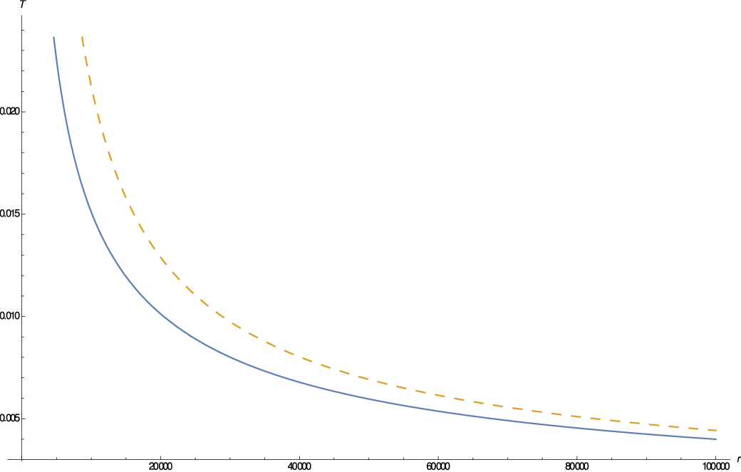
Figure 1 then gives the graphical behavior of the temperature when $\alpha=d=-1$ , $g(t)=t=0.5$ and $w(t)=-1$ .

We find that the temperature is decreasing as we approach the boundary and the causal temperature is greater than the Eckart temperature. This is consistent with other treatments (see for example the recent analysis of Reddy et al. [35]).

Refer to caption — Figure 1: Causal temperature (dashed line), noncausal temperature (solid line) versus $r$

Table 1: Symmetry, invariants, restrictions and resulting gravitational potentials

Symmetry	Invariants	Restrictions	Gravitational potentials
$aG_{1}+bG_{2}$	$x=\frac{\exp\left(\int^{t}\frac{dt}{af(t)}\right)}{r^{1/c}},$	$g=kh,b=0$	$A=\frac{n}{f(t)}\exp\left(\int^{x}\frac{8acx^{c-1}\exp\left(\frac{2ax^{c}}{ck}\right)\left(ax^{c}-ck\right)}{\exp\left(\frac{2ax^{c}}{ck}\right)\left(6a^{2}x^{2c}-10ackx^{c}+3c^{2}k^{2}\right)+m}\,dx+\int^{t}\frac{cdt}{af(t)}\right),$
$\qquad+cG_{3}$	$A=\frac{h(x)}{f(t)}$		$B=\frac{kf(t)}{\exp\left(\int^{t}\frac{cdt}{af(t)}\right)}A$ where $x=\exp\left(\int^{t}\frac{\,dt}{af(t)}\right)r^{-1/c}$
	$\times\exp\left(\int^{t}\frac{cdt}{af(t)}\right.$	$g=kh,b=-2c$	$A=\frac{n}{f(t)}\exp\left(\int^{x}\frac{8ac\exp\left(\frac{2ax^{-c}}{ck}\right)\left(ckx^{c}-a\right)}{x\left(\exp\left(\frac{2ax^{-c}}{ck}\right)\left[6a^{2}+3c^{2}k^{2}x^{2c}-10ackx^{c}\right]+mx^{2c}\right)}\,dx\right.$
	$\left.+\int^{t}\frac{bdt}{af(t)}\right),$		$\qquad\quad-\left.\int^{t}\frac{cdt}{af(t)}\right),$
			$B=\frac{kf(t)}{r^{2}\exp\left(\int^{t}\frac{-cdt}{af(t)}\right)}A,$ where $x=\exp\left(\int^{t}\frac{\,dt}{af(t)}\right)r^{-1/c}$
	$B=g(x)r^{b/c}$	$g=kh,b=-c$	$A=\frac{1}{f(t)}\left(m\left[r^{-1/c}\exp\left(\int^{t}\frac{dt}{af(t)}\right)\right]^{\frac{a\sqrt{3a+ck}}{2k\sqrt{a-ck}}}\right.$
			$\qquad\left.+n\left[r^{-1/c}\exp\left(\int^{t}\frac{dt}{af(t)}\right)\right]^{-\frac{a\sqrt{3a+ck}}{2k\sqrt{a-ck}}}\right){}^{\frac{2ck}{3a+ck}},$
			$B=\frac{kf(t)}{r}A$
		$g=kh,b=-c,$	$A=\frac{n}{f(t)}\frac{\left[r^{-1/c}\exp\left(\int^{t}\frac{dt}{af(t)}\right)\right]^{m}}{\exp\left(\frac{c^{2}}{48}\log^{2}\left[r^{-1/c}\exp\left(\int^{t}\frac{dt}{af(t)}\right)\right]\right)},$
		$k=\frac{-3a}{c}$	$B=\frac{-3a}{c}\frac{f(t)}{r}A$
$bG_{2}+cG_{3}$	$A=h(t)r^{(b+c)/c},$	$b=\left(\pm\frac{\sqrt{3}}{3}-1\right)c$	$A=\pm\frac{\sqrt{3}}{2}\frac{g^{\prime}\sqrt{g}}{\sqrt{g}+d}r^{\pm\frac{\sqrt{3}}{3}},$
	$B=g(t)r^{b/c},\text{ and }t$		$B=gr^{\pm\frac{\sqrt{3}}{3}-1}$
$aG_{1}+bG_{2}$	$A=h(r)\frac{\exp\left(\int^{t}\frac{bdt}{af(t)}\right)}{f(t)},$	$g=kh$	$A=\frac{d}{r^{4/3}f(t)}\left(\frac{\left(\alpha(r)+2a^{2}+abkr\right)^{2}}{\left(\alpha(r)+2abkr+a^{2}\right)}\right)^{1/3}\exp\left(\int^{t}\frac{bdt}{af(t)}-\frac{\alpha(r)}{3a^{2}}-\frac{bkr}{3a}\right),$
	$B=g(r)$		$B=kf(t)A$
	$\times\exp\left(\int^{t}\frac{bdt}{af(t)}\right),$		$A=\frac{d}{f(t)}\left(\frac{\alpha(r)+2abkr+a^{2}}{\left(\alpha(r)+2a^{2}+abkr\right)^{2}}\right)^{1/3}\exp\left(\int^{t}\frac{bdt}{af(t)}+\frac{\alpha(r)}{3a^{2}}-\frac{bkr}{3a}\right),$
	$\text{ and }r$		$B=kf(t)A$

Table 2: Equation of state

Symmetry	Gravitational potentials	Equation of state
$aG_{1}+bG_{2}$	$A=\frac{1}{f(t)}\left(m\left[r^{-1/c}\exp\left(\int^{t}\frac{dt}{af(t)}\right)\right]^{\frac{a\sqrt{3a+ck}}{2k\sqrt{a-ck}}}\right.$	$p_{\parallel}=\lambda\mu,$
$\qquad+cG_{3}$	$\qquad\left.+n\left[r^{-1/c}\exp\left(\int^{t}\frac{dt}{af(t)}\right)\right]^{-\frac{a\sqrt{3a+ck}}{2k\sqrt{a-ck}}}\right){}^{\frac{2ck}{3a+ck}},$	$\lambda=\frac{ack}{a^{2}-ack+c^{2}k^{2}}$
	$B=\frac{kf(t)}{r}A$
	$A=\frac{n}{f(t)}\frac{\left[r^{-1/c}\exp\left(\int^{t}\frac{dt}{af(t)}\right)\right]^{m}}{\exp\left(\frac{c^{2}}{48}\log^{2}\left[r^{-1/c}\exp\left(\int^{t}\frac{dt}{af(t)}\right)\right]\right)},$	$p_{\parallel}=\lambda\mu,$
	$B=\frac{-3a}{c}\frac{f(t)}{r}A$	$\lambda=-\frac{3}{13}$
$bG_{2}+cG_{3}$	$A=\pm\frac{\sqrt{3}}{2}\frac{g^{\prime}\sqrt{g}}{\sqrt{g}+d}r^{\pm\frac{\sqrt{3}}{3}},$	$p_{\parallel}=\lambda\mu,$
	$B=gr^{\pm\frac{\sqrt{3}}{3}-1}$	$\lambda=-\frac{2}{7}$

ACKNOWLEDGEMENTS

GZA and KSG thank the University of KwaZulu–Natal for continuing support. SDM acknowledges that this research is supported by the South African Research Chair Initiative of the Department of Science and Technology and the National Research Foundation.

References

[1] L. Herrera, A. Di Prisco, J. Martin, J. Ospino, N.O. Santos, O. Troconis, Phys. Rev. D 69, 084026 (2004)
[2] A. Di Prisco, L. Herrera, G. Le Denmat, M.A.H. MacCallum, N.O. Santos, Phys. Rev. D 76, 064017 (2007)
[3] L. Herrera, A. Di Prisco, E. Fuenmayor, O. Troconis, Int. J. Mod. Phys. D 18, 129 (2009)
[4] R. Chan, M.F.A. Da Silva, C.F.C. Brandt, Int. J. Mod. Phys. D 23, 145 (2011)
[5] G. Pinheiro, R. Chan, Gen. Relativ. Gravit. 45, 243 (2013)
[6] G. Pinheiro, R. Chan, Gen. Relativ. Gravit. 43, 1451 (2011)
[7] L. Herrera N.O. Santos, Gen. Relativ. Gravit. 42, 2383 (2010)
[8] G. Govender, M. Govender, K.S. Govinder, Int. J. Mod. Phys. D 19, 1773 (2010)
[9] K.S. Govinder M. Govender, Gen. Relativ. Gravit. 44, 147 (2012)
[10] G.Z. Abebe, S.D. Maharaj, K.S. Govinder, Gen. Relativ. Gravit. 46, 1733 (2014)
[11] A.M. Msomi, K.S. Govinder, S.D. Maharaj, J. Phys. A: Math. Theor. 43, 285203 (2010)
[12] A.M. Msomi, K.S. Govinder, S.D. Maharaj, Gen. Relativ. Gravit. 43, 1685 (2011)
[13] M.C. Kweyama, K.S. Govinder, S.D. Maharaj, Class. Quantum Grav. 28, 105005 (2011)
[14] M.C. Kweyama, K.S. Govinder, S.D. Maharaj, J. Math. Phys. 53, 033707 (2012)
[15] C.A. Kolassis, N.O. Santos, D. Tsoubelis, Astrophys. J. 327, 755 (1988)
[16] S. Thirukkanesh, S.D. Maharaj, J. Math. Phys. 50, 022502 (2009)
[17] M. Govender, S. Thirukkanesh, Int. J. Theor. Phys. 48, 3558 (2009)
[18] B.V. Ivanov, Gen. Relativ. Gravit. 42, 1835 (2012)
[19] L. Herrera, G. Le Denmat, N.O. Santos, A. Wang, Int. J. Mod. Phys. D 13, 583 (2004)
[20] S.D. Maharaj, M. Govender, Int. J. Mod. Phys. D 14, 667 (2005)
[21] L. Herrera, A. Di Prisco, J. Ospino, Phys. Rev. D 74, 044001 (2006)
[22] S.S. Misthry, S.D. Maharaj, P.G.L. Leach, Math. Meth. Appl. Sci. 31, 363 (2008)
[23] G.Z. Abebe, K.S. Govinder, S.D. Maharaj, Int. J. Theor. Phys. 52, 3244 (2013)
[24] B.C. Tewari, Astrophys. Space. Sci. 306, 273 (2006)
[25] B.C. Tewari, Gen. Relativ. Gravit. 45, 1547 (2013)
[26] N. Pant, R.N. Mehta, B.C. Tewari, Astrophys. Space. Sci. 327, 279 (2010)
[27] N. Pant, B.C. Tewari, Astrophys. Space. Sci. 331 645 (2011)
[28] L. Herrera, A. Di Prisco, J. Ospino, Gen. Relativ. Gravit. 42, 1585 (2010)
[29] Y. Nyonyi, S.D. Maharaj, K.S. Govinder, Eur. Phys. J. C 73, 2637 (2013)
[30] Y. Nyonyi, S.D. Maharaj, K.S. Govinder, Eur. Phys. J. C 74, 2952 (2014)
[31] G.Z. Abebe, S.D. Maharaj, K.S. Govinder, Gen. Relativ. Gravit. 46, 1650 (2014)
[32] A.K. Head, Comp. Phys. Comm. 71, 241 (1993)
[33] M. Govender, S.D. Maharaj, R. Maartens, Class. Quantum Grav. 15, 323 (1998)
[34] M. Govender, R. Maartens, S.D. Maharaj, Mon. Not. R. Astron. Soc. 310, 557 (1999)
[35] K. P. Reddy, M. Govender, S.D. Maharaj, Gen. Relativ. Gravit. 47, 35 (2015)