Rendezvous Missions to Temporarily-Captured Near Earth Asteroids

In this paper, the circular restricted three-body problem [18] is used to approximate the spacecraft dynamics. This is justified by the fact that a TCO can be assumed of negligible mass, and that the spacecraft evolving in the TCO’s temporary capture space is therefore attracted mainly by two primary bodies, the Earth and the Moon.

The CR3BP model is well known, let us however go through some notations fo the sequel of the paper. We denote by $(x(t),y(t),z(t))$ the spatial position of the spacecraft at time $t$. In the rotating coordinates system, and under proper normalization, the primary planet identified here to the Earth, has mass $m_{1}=1-\mu$ and is located at the point $(-\mu,0,0)$; while the second primary, identified to the Moon, has a mass of $m_{2}=\mu$ and is located at $(1-\mu,0,0)$, where $\mu=1.2153e-2$. The distances of the spacecraft with respect to the two primary bodies are given by $\varrho_{1}=\sqrt{(x+\mu)^{2}+y^{2}+z^{2}}$, $\varrho_{2}=\sqrt{(x-1+\mu)^{2}+y^{2}+z^{2}}$ respectively. The potential and kinetic energy, respectively $V$ and $K$ of the system are given by

We assume a propulsion system for the spacecraft is modeled by adding terms to the equations of motion depending on the thrust magnitude and some parameters related to the spacecraft design. The mass of the spacecraft is denoted by $m$. Under those assumptions, we have the following equations of motion:

where $u(.)=(u_{1}(.),u_{2}(.),u_{3}(.))$ is the control, and satisfies the constraint $\|u\|=\sqrt{u_{1}^{2}+u_{2}^{2}+u_{3}^{2}}\leq 1$, and with $T_{\rm max}/m$ normalized. A first integral of the free motion is given by the energy of the system $E=K-V$. We will later use this energy value to analyze the choice of the rendezvous point and the parking orbit for the spacecraft. It is well know that the uncontrolled motion of the dynamical system has five equilibrium points defined as the critical points of the potential $V$. Three of them $L_{1},L_{2}$ and $L_{3}$ are aligned with the Earth-Moon axis and have been shown to be unstable, while the two others are stable and are positioned to form equilateral triangles in the plane of orbit with the two primaries. Since our goal is to maximize the final mass we must include the differential equation governing the variation of the mass along the transfer:

where the parameter $\beta$, the thruster characteristic of our spacecraft, is given by $\beta=\frac{1}{I_{sp}g_{0}}$ (it is the inverse of the ejection velocity $v_{e}$), with $I_{\mathrm{sp}}$ the specific impulse of the thruster and $g_{0}$ the acceleration of gravity at Earth sea level.

Let $q=(q_{s},q_{v})^{t}$ where $q_{s}=(x,y,z)^{t}$ represents the position variables and $q_{v}=(\dot{x},\dot{y},\dot{z})^{t}$ the velocity ones. From section 2.1, our dynamical system is an affine control system of the form:

where the drift is given by $F_{0}(q)=(\dot{x},\dot{y},\dot{z},2\dot{y}+x-\frac{(1-\mu)(x+\mu)}{\varrho_{1}^{3}}-\frac{\mu(x-1+\mu)}{\varrho_{2}^{3}},-2\dot{x}+y-\frac{(1-\mu)y}{\varrho_{1}^{3}}-\frac{\mu y}{\varrho_{2}^{3}},-\frac{(1-\mu)z}{\varrho_{1}^{3}}-\frac{\mu z}{\varrho_{2}^{3}})^{t}$, and the control vector fields are $F_{i}(q)=\vec{e}_{3+i}$ with $\vec{e}_{i}$ forming the orthonormal basis of $\mbox{I\hskip-1.49994ptR}^{6}$.

We consider the rendezvous transfer from an initial point $q^{rdv}(t_{0})$ on a parking orbit $\mathcal{O}_{0}\in\mbox{I\hskip-1.49994ptR}^{6}$ to a final position and velocity $q^{rdv}(t_{f})$ on the 2006RH₁₂₀ orbit. Note that the initial and final positions and velocities are variables of the global optimization problem. The criterion to maximize is the final mass which is equivalent to minimizing the fuel consumption or the $\Delta v=\int_{t_{0}}^{t_{f}}\frac{T_{\max}\|u(t)\|}{m(t)}dt$. Since the mass evolves proportionally to the norm of the thrust, our criterion is equivalent to the minimization of the $L_{1}$-norm of the control:

where $\mathcal{U}=\{u(.);{\rm measurable\;bounded\;and}\;\|u(t)\|\leq 1\;{\rm for\;almost\;all}\;t\}$, $t_{0}$ and $t_{f}$ are respectively the initial and final time. Remark that since we choose $\mathcal{O}_{0}$ to be a Halo orbit around a libration point, it is uniquely determined by a single point of the orbit using the uncontrolled CR3BP dynamics. This fact will play an important role for one of the necessary optimality conditions below. The large number of variables in our problem significantly adds complexity to the search for a solution. In particular, in the case of free final time we expect an infinite time horizon with a control structure that mimics impulsive maneuvers. To simplify our optimal problem we have two options, either we fix the transfer time or we fix the structure of the control. If we fix the final time, the sensitivity of the shooting method can be addressed by using the solution of a smoother criterion than the $L_{1}$-norm, for instance the $L_{2}$-norm, and linking it to the target criterion by a continuation procedure, see [13]. In this paper, however, we take a different approach and decide to fix the structure of the control. In the sequel we focus on designing transfers associated to controls with a piecewise constant norm with value in $\{0,1\}$ and four switchings. More precisely, we consider control functions that are piecewise continuous such that there exists times $t_{0}\leq t_{1}\leq t_{2}\leq t_{3}\leq t_{4}\leq t_{f}$ with

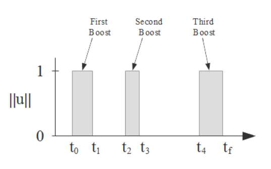
Here the final time $t_{f}$ is free. Note that our numerical method will be able to select the best control strategy even if it has less than three boosts.

The maximum principle provides first order necessary conditions for a trajectory to be optimal [26]. Details regarding the application of the maximum principle to orbital transfers can be found in many references, including [4, 26]. We denote by $X(t)=(q(t),m(t))\in\mbox{I\hskip-1.49994ptR}^{6+1}$ the state, where $q=(x,y,z,\dot{x},\dot{y},\dot{z})$ is the position and velocity of the spacecraft with $m$ its mass. The maximum principle applied to our optimal control problem states that if $(q(\cdot),m(\cdot),u(\cdot))=(X(\cdot),u(\cdot))$ is an optimal solution defined on $[t_{0},t_{f}]$, then there exists an absolutely continuous adjoint state $(p^{0},p_{X}(\cdot))=(p^{0},p_{q}(\cdot),p_{m}(\cdot))$, defined on $[t_{0},t_{f}]$ such that:

• •

  $(p^{0},p_{X}(\cdot))\neq 0,\ \forall t\in[t_{0},t_{f}]$, and $p^{0}\leq 0$ is a constant.

• •

  Let $H$, the Hamiltonian, be $H(t,X(t),p^{0},p_{X}(t),u(t))=p^{0}\|u(t)\|+\langle p_{X}(t),\dot{X}(t)\rangle$, then

  	$\displaystyle\dot{X}(t)=\frac{\partial H}{\partial p_{X}}(t,X(t),p^{0},p_{X}(t),u(t)),\ {\rm for\ a.e.}\ t\in[t_{0},t_{f}],$		(7)
  	$\displaystyle\dot{p}_{X}(t)=-\frac{\partial H}{\partial X}(t,X(t),p^{0},p_{X}(t),u(t)),\ {\rm for\ a.e.}\ t\in[t_{0},t_{f}],$		(8)

  where $\langle,\rangle$ denotes the inner product.

• •

  $H(t,X(t),p^{0},p_{X}(t),u(t))=\max_{\|\nu\|\leq 1}H(t,X(t),p^{0},p_{X}(t),\nu),\ \forall t$ s.t. $\|u(t)\|=1$ (maximization condition).

• •

  $\Psi(t_{i})=0$ for $i=1,\cdots,4$.

• •

  $H(t_{f},X(t_{f}),p^{0},p_{X}(t_{f}),u(t_{f}))=0$, if $t_{f}$ is free.

• •

  $\langle p_{q}(t_{0}),F_{0}(q(t_{0}))\rangle=0$ (initial transversality condition).

• •

  $p_{m}(t_{f})=0$.

The function $\Psi(\cdot)$ is the so-called switching function corresponding to the problem with an unrestricted control strategy and we have $\Psi(t)=p_{0}+T_{\mathrm{max}}\Big(\frac{\|p_{v}(t)\|}{m(t)}-p_{m}(t)\beta\Big)$.

The maximization condition of the Hamiltonian $H$ is used to compute the control on $[t_{0};t_{1}]\cup[t_{2};t_{3}]\cup[t_{4};t_{f}]$ and we have $u(t)=\frac{p_{v}(t)}{\|p_{v}(t)\|}\ {\rm for\;all}\;t\in[t_{0};t_{1}]\cup[t_{2};t_{3}]\cup[t_{4};t_{f}]$. The initial transversality condition reflects the fact that the initial departing point is free on the Halo orbit $\mathcal{O}_{0}$. Remark that since the data for the TCO’s trajectory are given as ephemerides, there are no dynamics equations to describe those orbits in the CR3BP. Thus, we cannot compute the tangent space to a TCO point and we cannot extract a transversality condition for $p_{q}(t_{f})$ at the rendezvous point. Since we expect numerous local extrema for this optimal control problem, it is however preferable to solve the problem for fixed rendezvous points on a discretization of the TCO orbit.

Our numerical method is based on the necessary conditions given in section 2.3. Let $Z(t)=(X(t),p_{X}(t)),\ t\in[t_{0};t_{f}]$, and $u(q,p)$ the feedback control expressed using the maximization condition. Then, we have $\dot{Z}(t)=\Phi(Z(t))$ where $\Phi$ comes from equations (7) and (8). The goal is to find $Z(t_{0})$, $t_{1}$, $t_{2}$, $t_{3}$, $t_{4}$ and $t_{f}$ such that the following conditions are fulfilled:

1. 1.

   $\Psi(t_{i})=0$ for $i=1,\cdots 4$;

2. 2.

   $X(t_{f})$ is the prescribed rendezvous point;

3. 3.

   $X(t_{0})\in\mathcal{O}_{0}$ and the initial transversality condition is verified;

4. 4.

   $H(t_{f})=0.$

The problem has been transformed into solving a multiple points boundary value problem. More specifically, we must find the solution of a nonlinear equation $S(Z(t_{0}),t_{1},t_{2},t_{3},t_{4},t_{f})=0$, where $S$ is usually called the shooting function. The evaluation of the shooting function is performed using the high order numerical integrator DOP853, see [15]. The search for a zero of the shooting function is done with the quasi-Newton solver HYBRD of the Fortran minpack package. Since $S(.)$ is nonlinear, the Newton-like method is very sensitive to the initial guess. This leads us to consider heuristic initialization procedures. We combine two types of techniques, a direct method and a continuation method. The discretization of the TCO’s orbit requires the study of thousands of transfers, we use a direct method for a dozen of rendezvous and expand to other points on the orbit using a continuation scheme. The motivation is that direct methods are very robust but time consuming while continuation method succeeded for our problem in most cases very rapidly. The direct method uses the modeling language Ampl, see [12], and the optimization solver IpOpt, see [28], with a second order explicit Runge-Kutta scheme. Details on advanced continuation methods can be found in [13] and [5], but we use a discrete continuation which is enough for our needs.

Moreover, note that in order to fulfill the initial transversality condition, we first prescribe $X(t_{0})$ on the parking orbit and find a zero of the shooting function satisfying all the other conditions. Afterward, we do a continuation on $X(t_{0})$ along the departing parking orbit in the direction that increases the final mass. Once a framing of the best $X(t_{0})$ with respect to the final mass is found, we perform a final single shooting to satisfy the initial transversality condition along with the other conditions. This decoupling in the search of an extremal is motivated by the fact that we could very likely find a local maximum on $X(t_{0})$ rather than a local minimum because of the periodicity of the initial parking orbit. We avoid this fact by first manually ensuring that the $X(t_{0})$ we find will be the one for the best final mass and not the worst. However, our continuation procedure on $X(t_{0})$ does not always succeed, mainly because of the high nonlinearity of the shooting function, as the trajectories we find can be very long. Even if some of the extremals we find do not satisfy the initial transversality condition with the aimed accuracy (typically a zero of the shooting function is deemed acceptable if $\|S(Z(t_{0}),t_{1,2,3,4,f})\|\leq 10^{-8}$), they are still rather close to satisfy it (of the order of $10^{-4}$).

The objective of this section is to present an analysis of the evolution of the fuel consumption with respect to the location of the rendezvous point on the 2006RH₁₂₀ orbit. As mentioned before, we restrict the study to transfers with at most three boosts. The primary goal is to obtain insights on the variation of fuel consumption based on the features of the rendezvous point such as its distance from $L_{2}$, or its energy. The spacrecraft characteristics are assumed to be an initial mass of $350\ kg$, a specific impulse $I_{\mathrm{sp}}$ of $230\ s.$ and a maximum thrust $T_{\mathrm{max}}$ of $22\ N$. The Halo orbit from which the spacecraft is departing is chosen to have a $z-$excursion of 5000 km around the EM libration point $L_{2}$, see Figure 3. The choice for this specific Halo orbit is motivated by the successful Artemis mission [22, 23] that used Halo orbits with similar characteristics. The point corresponding to the positive $z-$excursion is $q_{\mathrm{HaloL_{2}}}=(1.119,0,0.013,$ $0.,0.180,0)$, and the period of this particular Halo orbit is $t_{\mathrm{HaloL_{2}}}=3.413$ in normalized time units or approximatively $14.84\ days$.

During the period represented in Figure 1, asteroid 2006RH₁₂₀ does 17 clockwise revolutions around the origin of the CR3BP frame, and 3.6 revolutions in Earth inertial reference frame. The evolution of the energy of 2006RH₁₂₀ and its distance to the Earth-Moon libration point $L_{2}$ as the asteroid evolves on its orbit are given in Figure 4.

To analyze the variations of the fuel consumption with respect to the rendezvous point on the orbit, we discretize uniformly the orbit of 2006RH₁₂₀ using 6 hours steps. For each rendezvous point of this discretization, we compute an extremal transfer (i.e. a solution of the maximum principle) with free final time using the techniques explained in section 2. Figure 5 shows the evolution of the final mass, the $\Delta v$ and of the duration of the transfer with respect to the rendezvous point on the 2006RH₁₂₀ orbit for a spacecraft departing from the Halo $L_{2}$ orbit and corresponding to the three boosts control strategy. As explained in section 2.4, some of the departure point on the Halo orbit are not fully optimized – this is the case for about two thirds of them. Also note that a departure point different from $q_{\mathrm{HaloL_{2}}}$ implies a drift phase whose duration is not included in the transfer duration. It can be observed that the final mass has many local extrema and that the variation of the duration of the mission is not continuous (contrary to what we would expect). It is most likely due to local minima or to the fact that the value function of the problem can present discontinuities.

Figure 6 shows the evolution of the departure point on the hibernating orbit for the spacecraft with respect to the rendezvous point on 2006RH₁₂₀ (left) as well as the three most frequent departure points on the initial Halo orbit (right). More precisely, we represents the optimized argument of $(y,z)(0)$ (up to the quadrant: $arctan(z(0)/y(0))$). Note that the initial position on the Halo orbit directly depends on the optimized initial drift time. Since this initial drift phase has not always been successfully optimized, this figure has to be interpreted with caution. However, we can see that the departure position on the initial periodic orbit seems to always be close to a multiple of $\pi$.

Comparing the evolution of the final mass from Figure 5 and the evolution of 2006RH₁₂₀ energy from Figure 4, we can see that the best final masses are obtained on the first half of 2006RH₁₂₀ trajectory, that is for rendezvous points which energies are closer to the departing energy. For the best transfer, the energy difference between the rendezvous point on 2006RH₁₂₀ and the departing point on the Halo orbit is about 0.046. The rendezvous point with the closest energy to the initial orbit is only slightly before the optimal rendezvous point. Its final mass is 319.3 kg which is only 0.5 kg worst than the best final mass. This remark suggests strongly that a small difference in energy between the rendezvous point on 2006RH₁₂₀ orbit and the departing point for the spacecraft on the Halo orbit is advantageous.

The best transfer is represented on Figures 7, and some relevant data is also presented in Table 1.

This transfer has a $\Delta v$ of $203.6\ m/s$. The rendezvous takes place on June 26^th 2006 and lasts $415.5\ days$ which would require to detect and launch the mission about 14 months before June 1^st 2006.

On Figure 8, we display the orbit of 2006RH₁₂₀ in both the rotating and inertial frame with the rendezvous point for the best transfer.

The best transfer exhibits 14 revolutions around the origin (in the rotating frame) and has a significant variation in the $z-$coordinate with respect to the EM plane. In particular, the $z-$coordinate of the rendezvous point is $-1.04$ normalized units, that is about 400 thousand $km$, and the maximum $z-$coordinate along the trajectory is $5.34$ normalized units, that is about 2 million $km$. The departure point on the parking orbit occurs $4.5$ days after $q_{\mathrm{HaloL_{2}}}$. The control strategy consists of a first boost of $19.7\ s$, a second boost starting after $154.7\ days$ and lasting $51.1\ min$ , finally, the last boost starting $261.1\ days$ after the second boost and lasts $13.8\ s$, see Figure 9.

Despite a seemingly short initial boost, this trajectory does not exhibit the profile of an initial jump on an unstable invariant manifold. However, this trajectory exploits the fact that a small initial boost leads to a far location where the gravity field of the two primaries is small and where the second boost can efficiently aim at the rendezvous point. In particular, we expect the existence of other local minima with a larger final time, going further away from the initial and final positions and providing an even better final mass. Also note that this kind of strategy could not have been obtained if we had restricted the control structure to have two boosts rather than three.

To contrast with the best transfer we represent the worst transfer in Figures 10. This transfer has a $\Delta v$ of $962.5\ m/s$ (final mass is $m_{f}=228.4kg$) and a transfer time of $37.9$ days. The final position is $q_{p}^{\mathrm{rdv}}=(-0.65,0.35,0.92)$ and the final velocity is $q_{v}^{\mathrm{rdv}}=(-0.61,1.21,-0.28)$. The energy at the worst rendezvous point is about $-0.168$, and the maximum distance to $L_{2}$ is $6.21$ LD.

References

- [1] E. Belbruno and J. Miller, Sun perturbed earth-to-moon transfers with ballistic capture, Journal of Guidance and Control, vol. 16, no. 4, pp. 770-775, 1993.
- [2] C.R. Besette, D.B. Spencer, Optimal Space Trajectory Design: A Heuristic-Based Approach, Adavances in the Astronautical Sciences, Vol. 124, pp.1611-1628, 2006.
- [3] J.T. Betts, Practical Methods for Optimal Control Using Nonlinear Programming. Society for Industrial and Applied Mathematics, 2001.
- [4] J.B. Caillau, B. Daoud, J. Gergaud, Minimum fuel control of the planar circular restricted three-body problem. Celestial Mech. Dynam. Astronom. 114, no. 1, pp. 137-150, 2012.
- [5] J.B. Caillau, O. Cots and J. Gergaud, Differential continuation for regular optimal control problems. Optim. Methods Softw., 27, pp. 177-196, 2012.
- [6] M. Chyba, G. Patterson, G. Picot, M. Granvik, R. Jedicke, J. Vaubaillon, Designing Rendezvous Missions with Mini-Moons using Geometric Optimal Control. Journal of Industrial and Management Optimization, Vol. 10, Issue 2, pp. 477-501, 2014.
- [7] M. Chyba, G. Patterson, G. Picot, M. Granvik, R. Jedicke, J. Vaubaillon, Time-minimal orbital transfers to temporarily-captured natural Earth satellites. PROMS Series: Advances of Optimization and Control With Applications, Springer Verlag, 2014.
- [8] B.A. Conway, A Survey of Methods Available for the Numerical Optimization of Continuous Dynamic Systems, J Optim Theory Appl 152, pp. 271-306, 2012.
- [9] M. Pontani, B.A. Conway, Optimal Finite-Thrust Rendezvous Trajectories Found via Particle Swarm Algorithm, Journal of Spacecraft and Rockets, Vol. 50, No. 6, November-December 2013.
- [10] D.W. Dunham, R.W. Farquhar, N. Elsmont, E. Chumachenko, S. Aksenov, Y. Fedorenko, A. Genova, J. Horsewood, R. Furfaro, J. Kidd Jr, Using lunar swingbys and libration-point orbits to extend human exploration to interplanetary destinations, 64th International Astronautical Congress, Beijing, China, 2013.
- [11] D.C. Folta, T.A. Pavlak, A.F. Haapala, K.C. Howell, M.A. Woodard, Earth-Moon libration point orbit station keeping: Theory, modeling, and operations, Acta Astronautica, 2013.
- [12] R. Fourer, D.M. Gay, B.W. Kernighan, AMPL: A Modeling Language for Mathematical Programming, Duxbury Press, Brooks-Cole Publishing Company, 1993.
- [13] J. Gergaud, T. Haberkorn, P. Martinon, Low thrust minimum-fuel orbital transfer: a homotopic appoach, Journal of Guidance, Control and Dynamics, Vol.27, No.6, pp.1046-1060, 2004.
- [14] M. Granvik, J. Vauballion, R. Jedicke, The population of natural Earth satellites, Icarus, Volume 218, Issue 1, pp. 262-277, 2012.
- [15] E. Hairer, S.P. Norsett, G. Wanner, Solving Ordinary Differential Equations I. Nonstiff Problems. 2nd edition, Springer series in computational mathematics, Springer Verlag, 1993.
- [16] C.A. Kluever, Using Edelbaum’s Method to Compute Low-Thrust Transfers with Earth-Shadow Eclipses, Journal of Guidance, Control, and Dynamics, Vol. 34, No. 1, January-February 2011.
- [17] H. Kuninaka, K. Nishiyama, I. Funakai, Tetsuya, Y. Shimizu, J Kawaguchi, Asteroid Rendezvous of HAYABUSA Explorer Using Microwave Discharge Ion Engines IEPC-2005-10. Presented at the 29th International Electric Propulsion Conference, Princeton University, October 31 - November 4, 2005.
- [18] W.S. Koon, M.W. Lo, J.E. Marsden, S.D. Ross, Dynamical Systems, the Three-Body Problem and Space Mission Design, Springer-Verlag New York, 2011.
- [19] G. Mingotti, F. Toputto, F. Bernelli-Zazzera, Optimal Low-Thrust Invariant Manifold Trajectories via Attainable Sets, Journal of Guidance Control and Dynamics, Vol. 34, No.6, 2011.
- [20] G. Mingotti, P. Gurfil, Mixed Low-Thrust Invariant-Manifold Transfers to Distant Prograde Orbits Around Mars. Journal of Guidance, Control, and Dynamics, Vol. 33, No. 6, November-December 2010.
- [21] G. Mingotti, F. Topputo, F. Bernelli-Zazzera, A Method to Design Sun-Perturbed Earth-to-Moon Low-Thrust Transfers with Ballistic Capture, XIX Congresso Nazionale AIDAA, Forle, Italia, 17-21 September 2007.
- [22] C. Russell, V. Angelopoulos, The ARTEMIS Mission (Google eBook), Springer Science Business Media, Nov 18, 2013 - Science - 112 pages.
- [23] T.H. Sweetser, S.B. Broschart, V. Angelopoulos, G.J. Whiffen, D.C. Folta, M-K. Chung, S.J. Hatch, M.A. Woodard, ARTEMIS Mission Design. Space Science Reviews, Volume 165, Issue 1-4, pp. 27-57, December 2011.
- [24] M. Ozimek, K. Howell, Low-Thrust Transfers in the Earth-Moon System Including Applications to Libration Point Orbits, Journal of Guidance, Control, and Dynamics, Vol. 33, No. 2, March-April 2010.
- [25] G. Picot, Shooting and numerical continuation method for computing time-minimal and energy-minimal trajectories in the Earth-Moon system using low propulsion, Discrete Cont. Dyn. Syst. Ser. B, 17, pp. 245-269, 2012.
- [26] L. S. Pontryagin, V. G. Boltyanskii, R. V. Gamkrelidze and E. F. Mishchenko, The Mathematical Theory of Optimal Processes, John Wiley & Sons, New York, 1962.
- [27] M. Vaquero, K. Howell, Leveraging Resonant-Orbit Manifolds to Design Transfers Between Libration-Point Orbits, Journal of Guidance, Control, and Dynamics, Vol. 37, No. 4 (2014), pp. 1143-1157.
- [28] A. Waechter, L.T. Biegler, On the Implementation of an Interior-Point Filter-Line Search Algorithm for Large-Scale Nonlinear Programming, Research Report RC 23149, IBM T.J. Watson Research Center, Yorktown, New York, 2006.
- [29] K. Zhu, F. Jiang, J. Li, H. Baoyin, Trajectory Optimization of Multi-Asteroids Exploration with Low Thrust, Transactions of the Japan Society for Aeronautical and Space Sciences, Vol. 54, No. 175, pp.47-54, 2009.