$\mathcal{PT}$-symmetry breaking in the steady state of microscopic gain-loss systems

In 1998 Bender and Boettcher [1] described a class of non-Hermitian ‘Hamiltonians’ that exhibit a purely real energy spectrum, a surprising fact which they attributed to the underlying $\mathcal{PT}$ (parity- and time-reversal) symmetry. Their observation triggered considerable interest in discrete and continuous systems with $\mathcal{PT}$ symmetry along with alternative non-Hermitian formulations of quantum theory [2]. Such fundamental considerations remain speculative, but there exist many classical systems in which $\mathcal{PT}$-symmetric dynamics can be obtained with appropriately engineered loss and gain. This was first pointed out in the context of photonic waveguides [3, 4, 5, 6], lattices, and resonators [7, 8, 9, 10]. Other examples include cold atoms [11, 12, 13] and optomechanical devices [14, 15, 16]. Of particular interest in such systems is the $\it{breaking}$ of $\mathcal{PT}$ symmetry, i.e., when by tuning a parameter the energy spectrum becomes complex and the eigenvectors no longer exhibit the underlying $\mathcal{PT}$ symmetry. This phenomenon was first experimentally observed in optical waveguides [5, 6], and is currently the subject of intense experimental and theoretical research.

In this work we go beyond this dynamical picture and address an interesting and still open question: what are the steady states of actual physical systems with $\mathcal{PT}$ symmetry? This question becomes especially important for atomic or microscopic solid-state realizations of gain-loss systems. Here nonlinear saturation effects as well as the presence of thermal and quantum noise have a crucial influence on the system’s dynamics and the long-time behavior can no longer be inferred from an eigenvalue analysis only. By focusing on the experimentally relevant example of coupled mechanical resonators with optically-induced gain and loss (see Fig. 1) we show that $\mathcal{PT}$-symmetry breaking in the steady state exhibits various unexpected features and in general occurs via additional intermediate phases with retained or ‘weakly’ broken $\mathcal{PT}$ symmetry. Most importantly, we identify an unconventional transition from a high-noise balanced energy distribution to a parity-broken lasing state with strongly reduced fluctuations. This transition generalizes the phenomenon of $\mathcal{PT}$-symmetry breaking—hitherto defined only for eigenstates—to steady-state distributions of noisy systems. The mechanisms described here occur in systems of two coupled modes as well as in multi-resonator arrays, and will thus be of relevance for a large range of $\mathcal{PT}$ symmetric systems operated at low amplitudes and close to the quantum regime.

To motivate the following analysis by a concrete physical system, we consider a setup of two micromechanical resonators as shown in figure 1 a). The main findings discussed below, however, are more general and can be studied in other equivalent realizations, e.g., with coupled optical or microwave resonators. The mechanical resonators have a bare vibrational frequency $\omega_{\rm m}$ and they are mutually coupled, e.g., mechanically via the support, with strength $g$. In addition, optical or electrical cooling [17, 18, 19, 20, 21] and pumping [21, 22, 23, 24, 25, 26, 27, 28] schemes are used to induce mechanical loss for one resonator and an equal amount of mechanical gain for the other. In a frame rotating with $\omega_{\rm m}$, the semiclassical dynamics of the system is then described by the Itô stochastic differential equation [29, 30]

where $\alpha$ and $\beta$ are the dimensionless amplitudes of the pumped and cooled mode respectively (more details on the derivation of equation (1) are given in A).

The optically-induced gain and loss rates considered here are of the form

where $\Gamma$ is the maximal rate and $\sqrt{n_{0}}$ is the saturation amplitude. The value of $\nu$ characterizes the underlying heating or cooling mechanism and will be treated here as an adjustable parameter. For the three-level scheme depicted in figure 1 b) this parameter takes the value $\nu=2$ [21]. Instead, for conventional laser amplification with inverted two-level systems we would obtain $\nu=1$ [29]. Finally, $\gamma$ is the bare mechanical damping rate. Since we are interested in the $\mathcal{PT}$-symmetric limit (defined below), we assume $\gamma/\Gamma\rightarrow 0$. However, in all our calculations we retain a finite $\gamma>0$, which describes the actual physical situation and results in a well-defined steady state for all parameter regimes.

In equation (1) the (complex) stochastic forces $F_{\pm}(t)$ represent two independent white-noise processes with $\langle F_{\pm}^{*}(t)F_{\pm}(t^{\prime})\rangle=D_{\pm}\delta(t-t^{\prime})$. For resonators coupled to a reservoir of temperature $T$ the diffusion rates are $D_{+}(\alpha)=D_{\rm q}(\alpha)+2\gamma N_{\rm th}$ and $D_{-}=2\gamma N_{\rm th}$, where $N_{\rm th}=(e^{\hbar\omega_{\rm m}/k_{B}T}-1)^{-1}$. The contribution $D_{\rm q}(\alpha\rightarrow 0)=2\Gamma$ for the gain mode represents the intrinsic quantum noise associated with any amplification process and suggests that noise is a fundamental property of $\mathcal{PT}$-symmetric systems [31, 32, 33].

By ignoring the effect of noise and assuming $|\alpha|^{2},|\beta|^{2}\ll n_{0}$, equation (1) can be written as $\partial_{t}\psi=-iH\psi$, with a state vector $\psi=(\alpha,\beta)^{T}$ and a non-Hermitian ‘Hamiltonian’

This Hamiltonian is invariant under a combined parity ($\mathcal{P}$) and time-reversal ($\mathcal{T}$) symmetry for all values of $\Gamma/g$, where $\mathcal{P}:(\alpha,\beta)^{T}\leftrightarrow(\beta,\alpha)^{T}$ simply corresponds to an exchange of the two modes and $\mathcal{T}:i\rightarrow-i$. The eigenvalues and (unnormalized) eigenvectors of $H$ are [34] $\lambda_{\pm}=\pm\sqrt{g^{2}-\Gamma^{2}}$, $\psi_{+}=(e^{i\frac{\theta}{2}},e^{-i\frac{\theta}{2}})^{T}$ and $\psi_{-}=(ie^{-i\frac{\theta}{2}},-ie^{i\frac{\theta}{2}})^{T}$, where $\sin(\theta)=\Gamma/g$. We see that despite being non-Hermitian, for $\Gamma\leq g$ both eigenvalues $\lambda_{\pm}$ are real, indicating purely coherent oscillations between the two modes. In this regime of unbroken $\mathcal{PT}$ symmetry the eigenvectors are eigenstates of the symmetry operator, i.e., $\mathcal{PT}\psi_{\pm}=\psi_{\pm}$. For $\Gamma>g$, both eigenvalues become imaginary and correspond to a gain and a loss eigenmode. In this regime $\theta$ is complex and $\psi_{\pm}$ no longer possess the same symmetry as $H$. One thus speaks of a $\mathcal{PT}$-symmetry-breaking transition occurring at the (exceptional) point $\Gamma=g$ [2].

This conventionally studied $\mathcal{PT}$-symmetry-breaking effect captures the change in the system’s transient dynamics, as it is observed, e.g., in the propagation of coupled optical modes through an active medium with loss and gain [5, 6]. However, a simple eigenvalue analysis does not afford any conclusions concerning its steady state. Firstly, due to an exponentially amplified mode in the symmetry-broken phase, nonlinear effects must be taken into account in order to determine the system’s long-time behavior [4, 35, 36, 37, 38]. Secondly, due to non-decaying oscillations in the $\mathcal{PT}$-symmetric phase, any source of noise would heat up the system indefinitely, and within a linearized model the steady state would again be ill-defined.

Let us now return to the full model in equation (1) and evaluate the stationary state $\psi_{\rm ss}=(\alpha_{\rm ss},\beta_{\rm ss})^{T}$ in the absence of noise. Figures 2 a) and b) show the mode occupation numbers $|\alpha_{\rm ss}|^{2}$ and $|\beta_{\rm ss}|^{2}$ as a function of $\Gamma/g$, and for the two relevant cases $\nu=2$ and $\nu=1$. Firstly, we observe in both plots the expected transition at $\Gamma/g|_{\bf I\rightarrow II}=1$, below which (phase ${\bf I}$) the system dynamics is oscillatory with a small overall damping to $|\alpha_{\rm ss}|^{2}=|\beta_{\rm ss}|^{2}=0$ due to a finite $\gamma>0$. Above this transition point (phase II) the linearized system dynamics becomes unstable and both resonators reach a finite steady-state occupation number $|\alpha_{\rm ss}|^{2}/n_{0}=|\beta_{\rm ss}|^{2}/n_{0}=(\Gamma/g)^{1/\nu}-1+\mathcal{O}(\gamma)$, determined by the saturation of $\Gamma_{\pm}(\alpha)$. However, this steady state is still an eigenstate of the symmetry operator, $\mathcal{PT}\psi_{\rm ss}\propto\psi_{\rm ss}$, and contrary to our naïve expectation the system remains $\mathcal{PT}$-symmetric beyond the conventional transition point.

The existence of a $\mathcal{PT}$-symmetric steady-state with non-vanishing amplitude is permitted in models like the present one, where $\mathcal{PT}$-symmetry is retained even in the nonlinear regime. This means that a steady state $\psi_{\rm ss}$ with $|\alpha_{\rm ss}|=|\beta_{\rm ss}|\neq 0$ results in an equal suppression of both the gain and the loss rate, $\Gamma_{+}(\alpha_{\rm ss})=-\Gamma_{-}(\beta_{\rm ss})$ [see equation (2)]. This implies that there exists a symmetric state which satisfies $\dot{\psi}_{\rm ss}=0$ for all values of $\Gamma/g$. However, as one can see in figure 2, at larger values of $\Gamma$ the system eventually switches to a different, symmetry-broken state. As we discuss now, the details of this $\mathcal{PT}$-symmetry-breaking mechanism and the resulting state depend on the actual form of the saturable gain, which is here determined by the parameter $\nu$.

Considering first the case $\nu=2$, we find a second transition at $\Gamma/g=4$, beyond which (phase ${\bf III}$)

and the steady state breaks parity, i.e., $|\alpha_{\rm ss}|\neq|\beta_{\rm ss}|$. The $\mathcal{PT}$-symmetry-breaking point can be obtained from a linear stability analysis for phase II and for the present model we find

This result would imply the absence of symmetry breaking for $\nu=1$. Instead, for this case we observe a Hopf bifurcation around $\Gamma/g\approx 5.2$, beyond which the system approaches a limit cycle and undergoes periodic oscillations with the characteristic frequency $\omega_{\rm osc}\approx 2\sqrt{g^{3}(\Gamma-g)}/\Gamma$. The limit cycle is formed symmetrically around a central point $\psi_{\rm c}$ with $|\alpha_{\rm c}|=|\beta_{\rm c}|$, meaning that $\mathcal{PT}$-symmetry is preserved on average, but not at each point in time. To distinguish this behavior from the previous case we say that in this phase (${\bf IIIw}$) the $\mathcal{PT}$ symmetry is only ‘weakly’ broken. In contrast to full symmetry breaking, this transition is related to the finite asymmetry induced by $\gamma>0$, and would be hidden in the idealized models where $\gamma=0$. The value for the transition point is

independent of the precise value of $\gamma\ll\Gamma$. The general expressions in equations (5) and (6) show that for all intermediate cases, $1<\nu<2$, we obtain $1<(\Gamma/g)_{{\bf II}\rightarrow{\bf IIIw}}<(\Gamma/g)_{{\bf II}\rightarrow{\bf III}}<\infty$ and $\mathcal{PT}$-symmetry breaking occurs in three steps ${\bf I}\rightarrow{\bf II}\rightarrow{\bf IIIw}\rightarrow{\bf III}$. More details on the derivation of the above results and the stationary phases for general $\nu$ are given in B.

While similar nonlinear phenomena are in general expected for gain-loss systems [16, 37, 39, 40], our specific interest here is to understand the role of dynamical instabilities in the breaking of a steady-state symmetry. In particular, the above analysis shows that $\mathcal{PT}$-symmetry breaking occurs even in systems where the symmetry is fully retained in the nonlinear regime and a symmetric steady-state would be permitted in principle for all parameters.

We now show how the above picture changes in the presence of noise. For clarity we first restrict ourselves to a system which is dominated by thermal diffusion, i.e. $D_{\pm}=D=2\gamma N_{\rm th}$. For $\Gamma=0$ thermal noise induces additional amplitude fluctuations of about $(\Delta\alpha)^{2}\approx D/(2\gamma)=N_{\rm th}$, and we expect that as long as $N_{\rm th}<n_{0}$ the characteristic features shown in figure 2, which scale with the saturation number $n_{0}$, will only be smeared out, but not change significantly. This is confirmed numerically (not shown) and means that figure 2 is a good representation of the steady states of the system in the weakly nonlinear or low-noise regime. Therefore, we will now address the opposite regime $N_{\rm th}\gg n_{0}$.

Figure 3 a) shows the results of a numerical simulation of the stochastic equation (1), from which we obtain the steady-state distribution $P_{\rm ss}(\alpha,\beta)$ for $\nu=2$ and $N_{\rm th}/n_{0}=10$. In the following we write $\alpha=re^{i\theta_{\alpha}}$ and $\beta=ze^{i\theta_{\beta}}$ and make use of the fact that the system dynamics is invariant under a global phase rotation. The exact marginal distributions $P_{\rm ss}(\alpha)$ and $P_{\rm ss}(\beta)$ are then fitted by approximate distributions of the form

which allows us to extract a radial shift $r_{0}$ and $z_{0}$ and the range of fluctuations $(\Delta\alpha)^{2}$ and $(\Delta\beta)^{2}$ for both modes (see C). From these values plotted in figure 3 a) we see that the thermal noise now completely washes out the features associated with the $\mathcal{PT}$-symmetric phases I and II, and for a large range of $\Gamma$ the system reaches a steady state (phase ${\bf T}$), which is to a good approximation thermal, i.e., $r_{0}=z_{0}=0$ and $(\Delta\alpha)^{2}\simeq(\Delta\beta)^{2}\simeq N_{\rm th}$. Only after a critical value of $\Gamma/g|_{\bf T\rightarrow III}\approx 7.5$ are the fluctuations suddenly strongly suppressed. In this regime the system relaxes into an asymmetric coherent state with $r_{0}>z_{0}$ approximately given by the amplitudes $|\alpha_{\rm ss}|$ and $|\beta_{\rm ss}|$ given in equation (4) and $(\Delta\alpha)^{2},(\Delta\beta)^{2}\sim\gamma N_{\rm th}\Gamma/g^{2},\gamma N_{\rm th}/\Gamma\ll 1$.

Before we proceed, let us connect this transition to the phenomenon of $\mathcal{PT}$-symmetry breaking—hitherto defined only for individual states. To do so we introduce the $\mathcal{PT}$-symmetry parameter

which vanishes for a random set of states $\psi_{i}=(\alpha_{i},\beta_{i})^{T}$ if and only if each state satisfies $\mathcal{PT}\psi_{i}=e^{i\theta_{i}}\psi_{i}$, with some real phase $\theta_{i}$. Figure 3 b) shows that indeed $\Delta$ changes at the transition point from $\Delta\simeq\Delta_{\rm th}=0.215$ for a thermal state to $\Delta\rightarrow 1$ in the symmetry-broken phase. Note that also in the low-noise limit we obtain $\Delta=\Delta_{\rm th}>0$ in phase ${\bf I}$ and therefore only phase ${\bf II}$, where $\Delta\simeq 0$, has a strictly $\mathcal{PT}$-symmetric steady state.

One of the most striking features visible in figures 3 a) and c) is that in sharp contrast to a conventional lasing transition, the emerging coherent-state amplitudes after the $\mathcal{PT}$-symmetry breaking point are even smaller than the original level of thermal noise. This surprising effect can be understood as follows. Although at each instant in time the amplitudes $\alpha(t)$ and $\beta(t)$, and therefore the gain and loss rates $\Gamma_{+}(\alpha)$ and $\Gamma_{-}(\beta)$, can be quite different, the average dissipation rate $\bar{\Gamma}=\langle\Gamma_{-}-\Gamma_{+}\rangle_{\rm ss}$ when evaluated in the thermal phase vanishes, $\bar{\Gamma}\sim\mathcal{O}(\gamma)\sim 0$. What remains (on average) is the weak coupling to the high-temperature environment. In contrast, in the symmetry-broken phase we have $\langle|\alpha|\rangle_{\rm ss}\gg\langle|\beta|\rangle_{\rm ss}$. Therefore, there is a strong imbalance between loss and gain on average, i.e., $\bar{\Gamma}\sim\mathcal{O}(\Gamma)>0$, and the resulting net cooling effect suppresses fluctuations. Thus, this transition in the average dissipation rate of a stationary system can be seen as the counterpart of the transition from real to imaginary eigenvalues in the conventional definition of $\mathcal{PT}$-symmetry breaking. What we are still missing, however, is a simple criterion, which tells us why the system favors one or the other steady state.

To clarify the mechanism behind the symmetry-breaking transition we focus on the symmetry-broken regime $\Gamma/g\gg 1$, where we can assume that the amplitude of the gain mode $|\alpha(t)|\approx|\alpha_{\rm ss}|$ and the relative phase $\phi\simeq\pi/2$ are approximately constant. We then obtain the equation of motion for the amplitude of the loss mode, $z=|\beta|$ [41],

where $\langle\eta_{z}(t)\eta_{z}(t^{\prime})\rangle=\delta(t-t^{\prime})$ and (for $\gamma\rightarrow 0$)

The function $U(z)$ is an effective potential for $z$, which is sketched in Fig. 4 a). This potential has a local minimum at $z_{0}=|\beta_{\rm ss}|$ (corresponding to the steady state given in equation (4) for $N_{\rm th}\rightarrow 0$), which is separated by a finite barrier $\Delta U$ from the unstable region $z>z_{\rm max}$. In the presence of noise, a system initially located at $z\approx z_{0}$ can escape over this barrier via thermally activated processes with a characteristic rate $R_{\rm esc}\simeq R_{0}e^{-\frac{2\Delta U}{\gamma N_{\rm th}}}$, where $R_{0}=\sqrt{-U^{\prime\prime}(z_{\rm min})U^{\prime\prime}(z_{\rm max})/(4\pi^{2})}$ [30]. This rate increases as $\Gamma$ is reduced and once $R_{\rm esc}$ exceeds the bare damping $\gamma$, any configuration with fixed $\alpha$ and $\beta$ is rapidly destabilized and the transition to a quasi-thermal state with strongly fluctuating amplitudes occurs. In figure 4 b) we compare the transition point $\Gamma/g|_{\bf T\rightarrow III}$ obtained from the condition $\gamma=R_{\rm esc}$ with the numerically evaluated values for various $N_{\rm th}/n_{0}\gg 1$. The plot shows that $\mathcal{PT}$-symmetry breaking in the large-noise regime is very well described by this thermal activation model.

As it has been pointed out above, the implementation of any gain mechanism is necessarily accompanied by a minimum amount of quantum noise, $D_{\rm q}$, which ensures, e.g., the preservation of Heisenberg’s uncertainty relations in a quantum mechanical amplification process. For $\mathcal{PT}$-symmetric systems this implies that noise is not only an intrinsic property, but also that the symmetry in the gain and loss modes is broken on a fundamental level.

To illustrate the effect of pure quantum noise on the system’s steady state we set $N_{\rm th}=0$ and consider the quantum diffusion term

only. The assumed form of $D_{\rm q}(\alpha)$ applies for the three-level gain mechanism shown in figure 1, i.e., for the case $\nu=2$ (see A for additional details). Similar to the thermal noise limit discussed above we represent the resulting steady-state distributions for the loss and gain modes by the distribution maxima $r_{0}$, $z_{0}$ and the range of fluctuations $\Delta\alpha$ and $\Delta\beta$ respectively. The results are shown in figure 5 for a saturation parameter $n_{0}=10$. We see that while the steady-state distributions for low $\Gamma$ do no longer represent thermal states, there still exists a sharp transition between a high-noise $\mathcal{PT}$-symmetric phase and a $\mathcal{PT}$-symmetry-broken phase with strongly reduced fluctuations. Thus, we conclude that the $\mathcal{PT}$-symmetry-breaking mechanism identified above is not very sensitive to the details of the noise process and will exist in both thermal and quantum noise limited systems. Note that the semi-classical descriptions used in the current analysis is only valid for $n_{0}\gg 1$ while for $n_{0}\sim 1$ where quantum effects are most important a full quantum mechanical treatment must be employed. Such an analysis is, however, beyond the scope of the current work and will be presented elsewhere.

Finally, to show that $\mathcal{PT}$-symmetry breaking in the steady state exists also for extended systems, we generalize the analysis above to coupled resonator arrays with alternating gain and loss [42, 43], as depicted in figure 6 a). In this case the amplitudes $\alpha_{n}$ and $\beta_{n}$ for each unit cell obey

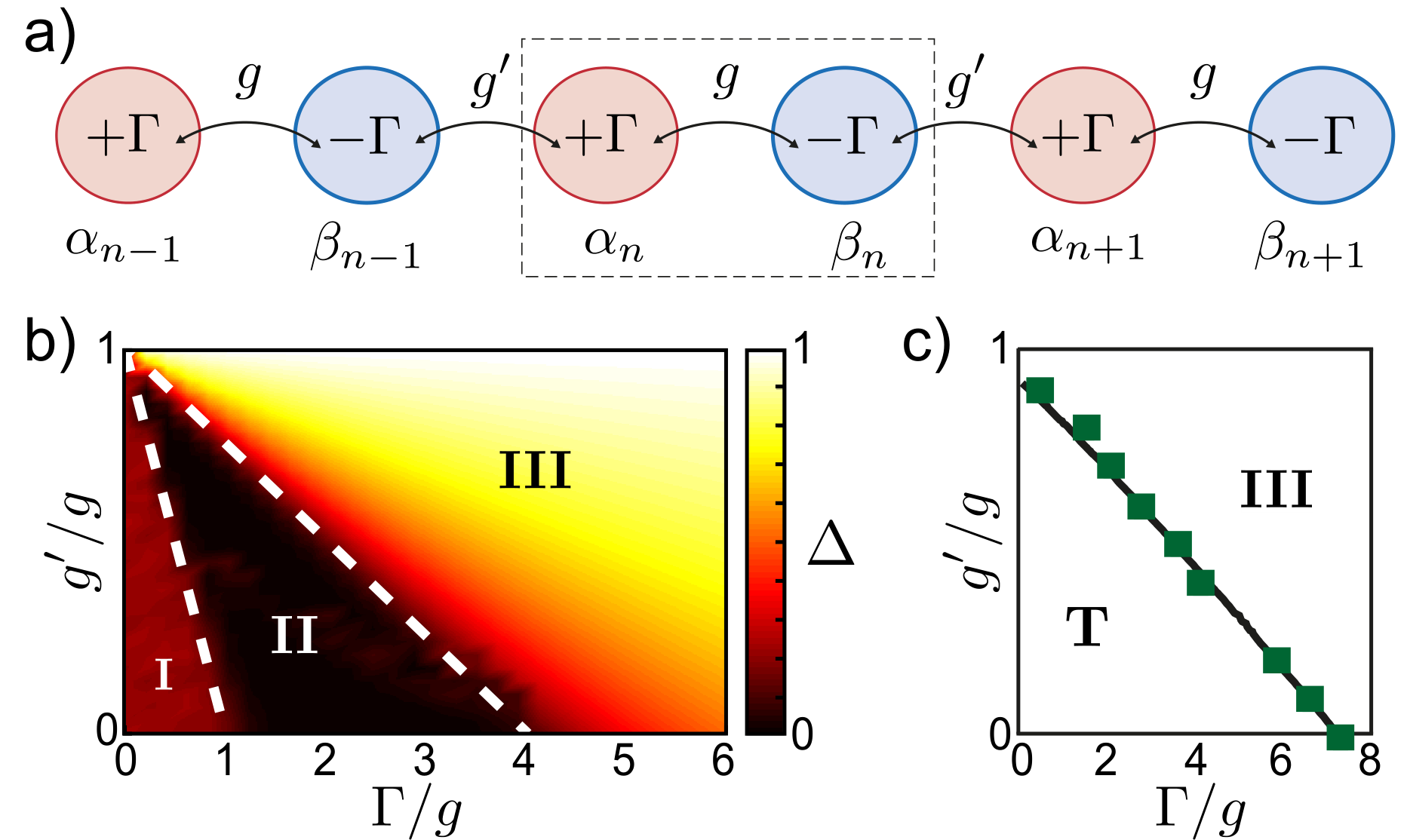
where $g^{\prime}$ is the coupling between the unit cells and $F_{n,\pm}(t)$ are independent thermal noise processes. Figure 6 summarizes the numerical results for the steady state of an array of $N=12$ resonators with periodic boundary conditions and $\nu=2$. The observed features can be understood from the plane wave ansatz [42, 44] $\alpha_{n}=A_{k}e^{ikn}$, $\beta_{n}=B_{k}e^{ikn}$, where $k=4\pi j/N$. This ansatz maps equation (12) onto a two-mode problem for $A_{k}$ and $B_{k}$, which is equivalent to equation (1), but with the replacement $g\mapsto g_{k}=|g+g^{\prime}e^{ik}|$. This implies that the largest ratio $\Gamma/|g_{k}|$ is always achieved for the $k=\pi$ mode [43], which therefore determines the symmetry-breaking properties of the array. For the special case $g=g^{\prime}$, i.e., $g_{k}=0$, the gain and the loss modes completely decouple, and $\mathcal{PT}$-symmetry breaking already occurs for $\Gamma\rightarrow 0$ [9]. For all intermediate parameters the phase boundaries in figure 6 are obtained from the analytic results for the two-mode problem, but with $g$ replaced by $g-g^{\prime}$. We see that the single-mode ansatz captures well the relevant physics both in the low- and high-noise regime. Note that, however, in the ‘thermal’ phase the behavior of the array can actually be much more complicated, since the system may undergo noise-induced jumps between multiple metastable configurations.

We have analyzed the breaking of $\mathcal{PT}$ symmetry in the steady state of coupled mechanical systems with loss and gain. We have shown how saturation effects and the influence of thermal or quantum noise lead to surprising new effects, which are not expected from the conventional eigenvalue analysis of idealized $\mathcal{PT}$-symmetric systems. These findings constitute a significant and important first step towards a general understanding of the behavior of realistic systems with $\mathcal{PT}$ symmetry, especially for systems operated close to the quantum regime or systems with strong nonlinearities.

References

- [1] C. M. Bender and S. Boettcher, ”Real Spectra in Non-Hermitian Hamiltonians Having Symmetry”, Phys. Rev. Lett. 80, 5243 (1998).
- [2] C. M. Bender, ”Making sense of non-Hermitian Hamiltonians”, Rep. Prog. Phys. 70, 947 (2007).
- [3] K. G. Makris, R. El-Ganainy, D. N. Christodoulides, and Z. H. Musslimani, ”Beam Dynamics in Symmetric Optical Lattices”, Phys. Rev. Lett. 100, 103904 (2008).
- [4] Z. H. Musslimani, K. G. Makris, R. El-Ganainy, and D. N. Christodoulides, ”Optical Solitons in Periodic Potentials”, Phys. Rev. Lett. 100, 030402 (2008).
- [5] A. Guo, G. J. Salamo, D. Duchesne, R. Morandotti, M. Volatier-Ravat, V. Aimez, G. A. Siviloglou, and D. N. Christodoulides, ”Observation of -Symmetry Breaking in Complex Optical Potentials”, Phys. Rev. Lett. 103, 093902 (2009).
- [6] C. E. Rüter, K. G. Makris, R. El-Ganainy, D. N. Christodoulides, M. Segev, and D. Kip, ”Observation of parity-time symmetry in optics”, Nature Phys. 6, 192 (2010).
- [7] A. Regensburger, C. Bersch, M.-A. Miri, G. Onishchukov, D. N. Christodoulides, and U. Peschel, ”Parity-time synthetic photonic lattices”, Nature 488, 167 (2012).
- [8] B. Peng, S. K. Özdemir, F. Lei, F. Monifi, M. Gianfreda, G. L. Long, S. Fan, F. Nori, C. M. Bender, and L. Yang, ”Parity-time-symmetric whispering-gallery microcavities”, Nature Phys. 10, 394 (2014).
- [9] L. Feng, Z. Jing Wong, R.-M. Ma, Y. Wang, and X. Zhang, ”Single-mode laser by parity-time symmetry breaking”, Science 346, 972 (2014).
- [10] H. Hodaei, M.-A. Miri, M. Heinrich, D. N. Christodoulides, and M. Khajavikhan, ”Parity-time-symmetric microring lasers”, Science 346, 975 (2014).
- [11] C. Hang, G. Huang, and V. V. Konotop, ” Symmetry with a System of Three-Level Atoms”, Phys. Rev. Lett. 110, 083604 (2013).
- [12] D. Haag, D. Dast, A. Löhle, H. Cartarius, J. Main, and G. Wunner, ”Nonlinear quantum dynamics in a -symmetric double well”, Phys. Rev. A 89, 023601 (2014).
- [13] T. E. Lee and C.-K. Chan, ”Heralded Magnetism in Non-Hermitian Atomic Systems”, Phys. Rev. X 4, 041001 (2014).
- [14] H. Jing, S. K. Özdemir, X.-Y. Lü, J. Zhang, L. Yang, and F. Nori, ”-Symmetric Phonon Laser”, Phys. Rev. Lett. 113, 053604 (2014).
- [15] X.-W. Xu, Y.-X. Liu, C.-P. Sun, and Y. Li, ”Mechanical symmetry in coupled optomechanical systems”, Phys. Rev. A 92, 013852 (2015).
- [16] X.-Y. Lü, H. Jing, J.-Y. Ma, and Y. Wu, ”-Symmetry-Breaking Chaos in Optomechanics”, Phys. Rev. Lett. 114, 253601 (2015).
- [17] I. Wilson-Rae, P. Zoller, and A. Imamoglu, ”Laser Cooling of a Nanomechanical Resonator Mode to its Quantum Ground State”, Phys. Rev. Lett. 92, 075507 (2004).
- [18] I. Martin, A. Shnirman, L. Tian, and P. Zoller, ”Ground-state cooling of mechanical resonators”, Phys. Rev. B 69, 125339 (2004).
- [19] F. Marquardt, J. P. Chen, A. A. Clerk, and S. M. Girvin, ”Quantum Theory of Cavity-Assisted Sideband Cooling of Mechanical Motion”, Phys. Rev. Lett. 99, 093902 (2007).
- [20] I. Wilson-Rae, N. Nooshi, W. Zwerger, and T. J. Kippenberg, ”Theory of Ground State Cooling of a Mechanical Oscillator Using Dynamical Backaction”, Phys. Rev. Lett. 99, 093901 (2007).
- [21] K. V. Kepesidis, S. D. Bennett, S. Portolan, M. D. Lukin, and P. Rabl, ”Phonon cooling and lasing with nitrogen-vacancy centers in diamond”, Phys. Rev. B 88, 064105 (2013).
- [22] S. D. Bennett and A. A. Clerk, ”Laser-like instabilities in quantum nano-electromechanical systems”, Phys. Rev. B 74, 201301(R) (2006).
- [23] D. A. Rodrigues, J. Imbers, and A. D. Armour, ”Quantum Dynamics of a Resonator Driven by a Superconducting Single-Electron Transistor: A Solid-State Analogue of the Micromaser”, Phys. Rev. Lett. 98, 067204 (2007).
- [24] J. Hauss, A. Fedorov, C. Hutter, A. Shnirman, and G. Schön, ”Single-Qubit Lasing and Cooling at the Rabi Frequency”, Phys. Rev. Lett. 100, 037003 (2008).
- [25] K. Vahala, M. Herrmann, S. Knünz, V. Batteiger, G. Saathiff, T. W. Hänsch, and Th. Udem, ”A phonon laser”, Nature Phys. 5, 682 (2009).
- [26] I. S. Grudinin, H. Lee, O. Painter, and K. J. Vahala, ”Phonon Laser Action in a Tunable Two-Level System”, Phys. Rev. Lett. 104, 083901 (2010).
- [27] J. Kabuss, A. Carmele, T. Brandes, and A. Knorr, ”Optically Driven Quantum Dots as Source of Coherent Cavity Phonons: A Proposal for a Phonon Laser Scheme”, Phys. Rev. Lett. 109, 054301 (2012).
- [28] I. Mahboob, K. Nishiguchi, A. Fujiwara, and H. Yamaguchi, ”Phonon Lasing in an Electromechanical Resonator”, Phys. Rev. Lett. 110, 127202 (2013).
- [29] D. F. Walls and G. J. Milburn, Quantum Optics (Springer-Verlag, Berlin Heidelberg, 1994 2008), 2nd ed.
- [30] C. Gardiner, Stochastic Methods (Springer-Verlag, Berlin Heidelberg, 2009), 4th ed.
- [31] H. Schomerus, ”Quantum Noise and Self-Sustained Radiation of -Symmetric Systems”, Phys. Rev. Lett. 104, 233601 (2010).
- [32] G. S. Agarwal and K. Qu, ”Spontaneous generation of photons in transmission of quantum fields in -symmetric optical systems”, Phys. Rev. A 85, 031802(R) (2012).
- [33] B. He, S.-B. Yan, J. Wang, and M. Xiao, ”Quantum noise effects with Kerr-nonlinearity enhancement in coupled gain-loss waveguides”, Phys. Rev. A 91, 053832 (2015).
- [34] H. Ramezani, T. Kottos, R. El-Ganainy, and D. N. Christodoulides, ”Unidirectional nonlinear -symmetric optical structures” Phys. Rev. A 82, 043803 (2010).
- [35] D. A. Zezyulin and V. V. Konotop, ”Nonlinear Modes in Finite-Dimensional -Symmetric Systems”, Phys. Rev. Lett. 108, 213906 (2012).
- [36] Y. Lumer, Y. Plotnik, M. C. Rechtsman, and M. Segev, ”Nonlinearly Induced Transition in Photonic Systems”, Phys. Rev. Lett. 111, 263901 (2013).
- [37] N. V. Alexeeva, I. V. Barashenkov, K. Rayanov, and S. Flach, ”Actively coupled optical waveguides”, Phys. Rev. A 89, 013848 (2014).
- [38] I. V. Barashenkov, D. E. Pelinovsky, and P. Dubard, ”Dimer with gain and loss: Integrability and PT-symmetry restoration”, J. Phys. A: Math. Theor. 48, 325201 (2015).
- [39] B. Peng, S. K. Özdemir, S. Rotter, H. Yilmaz, M. Liertzer, F. Monifi, C. M. Bender, F. Nori, and L. Yang, ”Loss-induced suppression and revival of lasing”, Science 346, 328 (2014).
- [40] M. Brandstetter, M. Liertzer, C. Deutsch, P. Klang, J. Schöberl, H. E. Türeci, G. Strasser, K. Unterrainer, S. Rotter, ”Reversing the pump dependence of a laser at an exceptional point”, Nature Commun. 5, 4034 (2014).
- [41] An equivalent analysis predicts a single stable minimum for the gain mode and much lower thermal activation rates for the relative phase .
- [42] N. Lazarides and G. P. Tsironis, ”Gain-Driven Discrete Breathers in -Symmetric Nonlinear Metamaterials”, Phys. Rev. Lett. 110, 053901 (2013).
- [43] O. Vazquez-Candanedo, J. C. Hernandez-Herrejon, F. M. Izrailev, and D. N. Christodoulides, ”Gain- or loss-induced localization in one-dimensional -symmetric tight-binding models”, Phys. Rev. A 89, 013832 (2014).
- [44] M.C. Cross and P. C. Hohenberg, ”Pattern formation outside of equilibrium”, Rev. Mod. Phys. 65, 851 (1993).
- [45] C. W. Gardiner and P. Zoller, Quantum Noise (Springer-Verlag, Berlin Heidelberg, 1991 2000), 2nd ed.
- [46] S. H. Strogatz, Nonlinear Dynamics and Chaos (Addison-Wesley Publishing Company, 1994).
- [47] The leaders of the MatCont project are W. Govaerts and Y. A. Kuznetsov, and as of publication the software is available at http://sourceforge.net/projects/matcont/.