Dust and Gas in the disk of HL Tauri:
Surface density, dust settling, and dust-to-gas ratio
Abstract
The recent ALMA observations of the disk surrounding HL Tau reveal a very complex dust spatial distribution. We present a radiative transfer model accounting for the observed gaps and bright rings as well as radial changes of the emissivity index. We find that the dust density is depleted by at least a factor of 10 in the main gaps compared to the surrounding rings. Ring masses range from 10–100 M⊕ in dust, and we find that each of the deepest gaps is consistent with the removal of up to 40 M⊕ of dust. If this material has accumulated into rocky bodies, these would be close to the point of runaway gas accretion. Our model indicates that the outermost ring is depleted in millimeter grains compared to the central rings. This suggests faster grain growth in the central regions and/or radial migration of the larger grains. The morphology of the gaps observed by ALMA - well separated and showing a high degree of contrast with the bright rings over all azimuths - indicates that the millimeter dust disk is geometrically thin (scale height 1 AU at 100 AU) and that a large amount of settling of large grains has already occurred. Assuming a standard dust settling model, we find that the observations are consistent with a turbulent viscosity coefficient of a few . We estimate the gas/dust ratio in this thin layer to be of the order of 5 if the initial ratio is 100. The HCO+ and CO emission is consistent with gas in Keplerian motion around a 1.7 star at radii from AU.
Subject headings
stars: individual (HL Tau) – protoplanetary disks – stars: formation – submillimeter: planetary systems – techniques: interferometric – radiative transferI. Introduction
Planet formation within disks around young stars requires the growth of sub-micron dust grains over many orders of magnitude. The dust feeding the disk in its early evolution is thought to have grown from the submicron grains typical of the interstellar medium, up to micron sized particles in the dense regions of molecular clouds and cores [43, e.g.]. Once incorporated into the disk, these grains must then grow from micron-sized to pebbles and ultimately kilometer-sized bodies. This extensive growth phase can only occur in the highest density regions of a protoplanetary disk – at or close to the disk’s midplane [14, 56].
The gas drag acting on the dust as it orbits the central star causes it to settle rapidly to the midplane. Just how much remains a poorly constrained quantity by direct observations. The small dust particles ( 1 m), best traced by scattered light, remain coupled tightly to the gas, while the larger particles, best studied at longer wavelengths, move toward the midplane. The thickness of the midplane depends on the balance between vertical settling and counter-acting stirring mechanisms [23, 17, 22]. Once in the midplane, particles are also expected to drift radially inward as a result of the combined action of the stellar gravity, the gas drag and the radial pressure gradient [4, 7]. The presence of planets within the disk further complicates the dynamics of the dust grains as they may create gaps whose profile depends on the planet mass, density profile, and grain size [42, 20, 24].
Fitting multi-color scattered light images of edge-on disks indicates the presence of stratification, with smaller grains found higher up in the disk atmosphere while larger grains have settled deeper [45, 50, 16, e.g.], as predicted by models. Tracing the properties of the dust layers deep inside the disk requires observations at long (millimeter) wavelengths where the disk becomes optically thin. Several multi-wavelength studies are now suggesting that the larger grain abundances depend on radius, with a concentration toward the center of protoplanetary disks [51, 28, 44, 38]; however, the spatial resolution was insufficient to resolve the vertical structure of the dust layer. In general, the midplane region of disks remains poorly constrained by direct observations.
HL Tau is a T Tauri star of spectral energy distribution (SED) Class I–II in the Taurus molecular cloud, at a distance of 140 pc. The disk has been widely studied in the (sub-)millimeter wavelength continuum [6, 41, 57, 35, 10, 36, 26, 32, 54]. The highest resolution millimeter observations so far [32] revealed a 120 AU dust disk and suggested, with comparison with the SED, that the millimeter grains may have already settled to the midplane. In addition to the disk structure, an orthogonal optical jet and a molecular bipolar outflow [40, e.g.] and an envelope [37, 52] have been reported.
HL Tau was recently observed with ALMA using baselines up to 15 km at wavelengths from 0.8-3 mm, which resulted in spatial resolutions down to 3.5 AU [2, hereafter 2]. These data provide the critical angular resolution needed to study the details of the disk midplane. They indicate the presence of numerous gaps and rings.
Here we model the recent ALMA data at all three wavelengths, in order to reproduce the main features of the HL Tau disk. We interpret the results in terms of the underlying dust distribution and evolution. We investigate whether a single unified dust model can reproduce both the ALMA images and SED, and compare the dust and gas disk also observed by ALMA.
II. Observations
HL Tau was observed as a science verification target within the ALMA Long Baseline Campaign; full details of the observations are given in 2 and [1]. The band 3, 6, and 7 calibrated continuum data sets and CLEANed images were downloaded from the ALMA Science portal11 1 http://www.almascience.org/, together with the tables for self-calibration, which we applied to the data.
From the images, the observed brightness in each band, and the spectral index profiles measured along the disk major axis are presented in Figure 1. A similar structure of alternating bright rings and dark gaps is seen in all three bands. The spectral index measured between 0.87 and 2.9 mm (lower panel) displays a significant increase from the inner regions to the outer disk, from 2.2 to 3.5, indicating a radial change in the spatially convolved dust emissivity and/or optical depth. The combined cleaning of the band 6 and 7 data [2] yields a higher resolution spectral index map, and a cut through this along the major axis is presented in the middle panel in Figure 1. As noted previously, this shows that the optical depths are significant in the rings at these shorter wavelengths, with sharp increases in the spectral index inside the gaps. In order to extract the underlying dust structure, we reproduce the data at all three wavelengths, and then compare the models with these radial profiles. Any differences in the derived models would then suggest evidence of a radial change in the dust characteristics.
The calibrated spectral line data sets in band 3 for 12CO =1-0 and HCO+ =1-0 were also downloaded and CLEANed. The default CLEAN parameters and taper from 2 were used for HCO+ giving a resolution of 0.25 arcsec. For the CO data set, CLEANing with a taper giving a spatial resolution of 0.2 arcsec was found to be a good compromise between resolving the disk and obtaining enough signal/noise per beam. Although the SNR of the spectral line data sets is relatively low and suffers from contamination at ambient cloud velocities, we were able to compare the results with a simple Keplerian disk in order to investigate the gas distribution.
III. Continuum modeling approach
To model the ALMA continuum data, we use the radiative transfer code MCFOST [49, 46]. Because of the remarkable symmetry of the ALMA images, we assume an axisymmetric, i.e. two-dimensional (2D), density structure. In particular, we ignore the slight offsets and change of inclinations of the rings compared to the central star [2]. We use standard disk parameters to describe the disk structure [e.g. 48, 3, see Section III.1] except for the surface density which shape is let free and is fitted for. Our aim is to determine whether such a simple model of the disk density structure can reproduce the main features observed by ALMA. Due to the complexity of the ALMA data sets, we build the model of surface density from the images and checked a posteriori by calculating a that the model and observed visibilities were in good agreement.
III.1. Radiative transfer model
We assume a flared gas density structure with a Gaussian vertical profile where is the distance from the star in the disk midplane and is the altitude above the midplane. For the gas disk scale height , we use a power-law distribution where is the scale height at radius AU. To keep the problem tractable, we fix some parameters and explore the parameter space in terms of surface density and dust settling. The disk scale height is set to 10 AU to be consistent with models of thermally supported disks (e.g. 11). is the disk flaring exponent, which we set to 1.15, again consistent with typical disk models. The exact values of and do not strongly affect the final conclusions and the defined gas disk structure is very close to hydrostatic equilibrium (see Appendix B). The inner radius is set to the dust sublimation radius. The outer radius is set to 150 AU, i.e. large enough that the surface density reaches negligible values at this distance from the star and in agreement with the size of the observed disk.
A surface density distribution per grain size is then fitted at each wavelength independently, using the procedure described below (Section IV.1).
Dust settling is implemented by describing the dust transport by turbulence as a diffusive process. This was shown to be a reasonable approximation to global MHD simulations of stratified and turbulent disks [21]. The degree of dust settling is set by varying the turbulent viscosity coefficient [53]. We assume that the gas vertical profile remains Gaussian and that the diffusion is constant vertically and given by , where is the midplane sound speed, is the gas scale height, and is the Schmidt number, which we fix to 1.5. The vertical density profile for a grain of size is given by equation 19 of [21]:
| (1) |
with , and the dust stopping time, where is the dust material density and is the gas density in the midplane. The density is finally normalized so that
| (2) |
We assume passive heating and fix the properties of the central star to K and [37]. We use a central mass M⊙, as derived from the CO and HCO+ observations (see Section V).
We adopt a fixed dust mixture composed of 60 % silicate [15], 15 % amorphous carbon [61], and 25 % porosity, although the details of the dust composition do not affect the results presented in this paper. We use a grain size distribution between and . and are set to m and 3 mm and we initially use (integrated over the whole disk). However, note that and are both modified locally due to the dust settling and varying surface density as a function of grain size. Each grain size is represented by a distribution of hollow spheres with a maximum void fraction of .


In summary, we fixed most of the model parameters, and focused our analysis on the parameters that are mainly probed by the new ALMA data: the disk surface density per grain size and dust settling via the parameter.
III.2. Building a model of the HL Tau disk
The construction of the 2D disk density structure was performed in two successive steps. First, we build the surface density of the model by reproducing the brightness distribution along the major axis, where the line-of-sight confusion due to the projection of the vertical structure is minimal. This procedure is repeated for the three ALMA bands and the resulting surface densities, which correspond to various grain sizes, are combined in a single model. In a second step, the vertical distribution is explored by modeling the complete 2D data sets and quantitatively comparing the synthetic and observed visibilities. The final model shows residuals smaller than the map rms, and visibilities in very good agreement, indicating that the model resulting from this procedure can account for most of the observed features in the ALMA data sets.
To obtain a surface density profile that matches the observed images, we use an iterative procedure. We first extract a brightness profile along the major axis of the disk in the CLEANed map and take an average of both sides. Because the model will be convolved before comparison with observations, we deconvolve the extracted brightness profile by a Gaussian beam whose FWHM corresponds to the projected FWHM along the disk semi major-axis of the observed 2D beam. This deconvolved brightness profile is then converted to a surface density profile assuming an initial power-law radial temperature profile (exponent = -0.5) consistent with the radial temperature dependence in typical disk models [12, 18, 47]. The assumption of power-law temperature with exponent -0.5 is needed only for to the first iteration, is calculated for all subsequent iterations. Using this initial surface density profile, we compute a model using MCFOST, convolve it with the corresponding beam, and extract a model brightness profile along the major axis. The surface density at any point in the disk is then corrected by the ratio of the observed profile divided by the model profile. To avoid too many oscillations in this procedure, this ratio is limited between 0.8 and 1.2. The procedure is iterated until the model brightness profile does not change by more than 1 % at any radius. The procedure requires of the order of 30 iterations to reach convergence.
Note that the procedure breaks down in the very inner regions of the disk due to high optical depth and because the central beam encloses all the azimuthal angles. For the first five central AU, we fixed instead a power-law surface density profile. We find that a slope of -0.5 reproduces well the brightness distribution of the outer parts of the central peak, but the exact value is not well constrained because the region is only partially resolved.
Despite exploring a range of parameter space for both the disk geometry and the dust properties, we could not reproduce the compact and peaked emission at the position of the star. Because the emission in the central peak is optically thick, we conclude that an additional unresolved source such as coronal free-free emission or extra heating due to accretion might be present close to the the star. We added the required unresolved emission at the position of the star in the model maps: 1.57, 1.90, and 2.59 mJy at band 3, 6 and 7 respectively. This represents 2 %, 0.2 % and 0.1 of the total flux in bands 3, 6, and 7 respectively. Note that the relative contribution of this additional emission in the central beam is not well constrained and depends on the model parameters: the non-resolved contributions cannot be large, but their exact value should be taken with caution.
For the iterative procedure, model images were produced by convolving the MCFOST images by a Gaussian beam of equivalent FWHM. The final simulated visibilities and images were produced by applying a modified version of the CASA simulator to the model. This computes the model visibilities at the exact same (,) coordinates as the observations using the ft task. To compute the model visibilities, we first average the observed data in time (using 300s bins) and in frequency to obtain one single continuum channel per available spectral window. This was performed to reduce the number of (,) points and corresponding computing time of the CASA simulator. The thermal noise at each wavelength was set using the median value of the precipitable water vapor (PWV) of the observations: 1.3, 0.65, and 0.54 mm at bands 3, 6, and 7 respectively. The resulting data set of model visibilities was CLEANed using the same parameters as for the observations, and the observed and modeled images were compared for consistency (Figure 2). We estimate the quality of the model by calculating a between the observed and synthetic visibilities. After binning, we have 229 910, 420 668 and 571 960 visibilities in bands 3, 6, and 7 respectively. were computed using the formal uncertainties from the interferometric weights, to which we added quadratically a 10 % calibration uncertainty. The from the three individual bands bands were added to compute the final . Our final model has a total of 1282. For the final model, visibilities were also computed without performing any time averaging, and we checked that the reconstructed simulated images almost did not show any difference, and that the were not affected by more than 2 %.
IV. Results from modeling
IV.1. Surface density profile and radial concentration of large grains
Figure 3 shows the resulting surface densities obtained by inverting the brightness profiles of the best models for the different wavelengths. The surface density profiles derived from observations in the three ALMA bands are broadly consistent with each other, suggesting that our basic modeling assumptions are also correct. In particular, we find that the central peak as well as the two most central rings are marginally optically thick, even at 2.9 mm (Figure 3), while the outermost broad ring becomes optically thin. The surface density extracted from the Band 6 data is also in good agreement with the analytical surface density derived by [32] and [33] from CARMA observations at the same wavelength (green dashed line in Figure 3, in the bright rings, the gaps were not detected by CARMA). In particular, our procedure recovers the transition between the power-law description and exponential tapering at radii larger than AU, as well as the shape of surface density in both regimes.
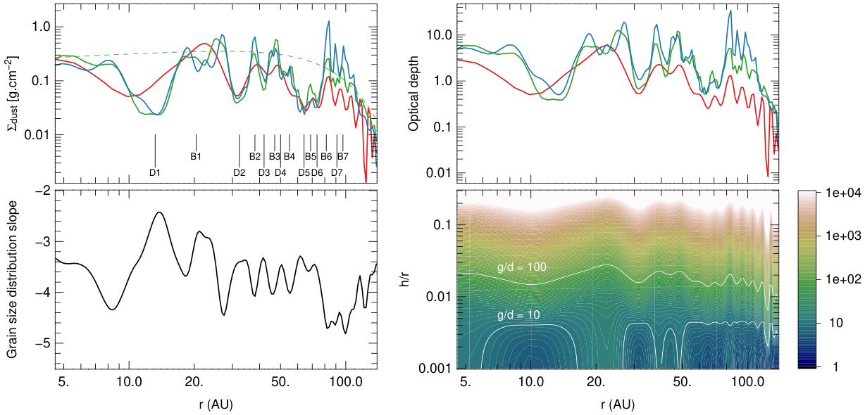
Interestingly, assuming a grain size distribution slope of , the surface density profiles we derive from the three bands start to differ significantly in the outermost ring, where the estimated surface density decreases as a function of wavelength. A model with a steeper slope, , results in similar surface density profiles at all bands in the outer ring, but the densities now differ significantly in the central regions. This suggests that grains larger than a fraction of a millimeter are depleted in the outer ring compared with the rest of the disk, supporting the idea that grain growth is less efficient in this part of the disk or that in the event of grain growth, radial migration has already effectively removed a significant fraction of the large grains. This can be observed directly by comparing the visibility curves at each wavelength (see bottom left panel of Figure 2). The shorter the wavelength, the faster the visibilities approach 0 as the baseline increases, indicating that the emission is getting more and more compact as the wavelength increases. Because the central rings are optically thick, this change in the derived surface density as a function of wavelength could, at least partly, also be due to the difference in optical depths. However, we explored several models, changing the dust distribution, but could not find a model that reproduces the surface density profile at all wavelengths, without invoking a change of the dust distribution as a function of the position.
To build a single model that reproduces the three bands simultaneously, we adopt a procedure similar to the one used in [45] and [24]. We use the three previously derived surface densities and assign each of them to a single grain size, which emits most at the corresponding wavelength: the surface densities from bands 3, 6, and 7 were used to define the distribution of the grains of size 0.4, 0.18, and 0.11 mm respectively. For intermediate sizes, the spatial distributions are interpolated in logarithm of the grain size. Outside of the range 0.11-0.40 mm, we do not extrapolate the distributions: all the grains smaller than 0.11 mm have the same surface density distribution, independently of their size. Similarly, all the grains larger than 0.40 mm have the same surface density distribution. Because a given grain size does not emit only in one given ALMA band, the final model does not show a as good agreement as the individual models only fitting one wavelength. However, the emissivity as a function of wavelength of a given grain size remains peaked enough so that the contamination between bands remains limited and the general agreement is good at all wavelengths (Figure 2). The size distribution at any point is no longer a power-law. In bottom left panel of Figure 3, we show the slope that fits best the local (integrated vertically) grain size distribution. The grain distribution has a local slope close to -3.5 up to 75 AU, while it approaches -4.5 between 75 and 120 AU, supporting the idea of depletion of large grains. The total dust mass of the best model is 5 10-4 M⊙.
Table 1 summarizes the properties of the various rings. The ring masses range from 7 to 120 M⊕. We use the same nomenclature as in 2 to name the gaps and rings. The ring masses are calculated by integrating the mass between two successive gaps, and the temperatures are the mass averaged dust temperatures. Uncertainties on the gap masses were computed by varying the gap depth, i.e. by multiplying the surface density in the gap by a constant without varying its shape. This procedure was repeated for various values of the constant until the gap was infinitely deep (the surface density virtually reaches 0 in the gap) and until it disappeared (the surface density in the gap reaches the interpolation between the rings). For each of these models, synthetic MCFOST images were calculated, visibilities computed using the CASA simulator and the total calculated. Due to the computing cost of the procedure (dominated by the calculations of the visibilities in CASA), a full Bayesian analysis taking into account the potential correlations between the densities in the various gaps and rings is out of reach with current computing facilities. Instead, we explored the mass of each gap independently. This approach allowed us to get an estimate of the uncertainties on the gaps (and rings) masses. In Table 1, we report the interval range where the remains smaller than 1.5 the minimum value. We find that this threshold corresponds to visible differences in the binned visibility curves as well as residuals above 3 in the CLEAN maps. Note that the central peak and ring B1 are optically thick even at 3 mm, so the corresponding mass estimates are lower limits.
The dust opacity and spectral index for each ring are computed for the integrated dust population in each ring (Table 1). The absolute values of the opacity result from our choice of dust properties and should be considered with an uncertainty of a factor a few. The outer rings display smaller opacities at 1 mm and spectral index (from 1 in the central rings to 1.3-1.4 in the two outer rings B6 and B7) due to the steeper grain size distribution and relative lack of millimeter-sized dust grains. Note that the change in opacity index between the inner and outer rings is smaller than the observed change in spectral index (bottom panel of Figure 1), as the low observed spectral index in the central regions of the disk results from a combination of the lower opacity index and high optical depth effects.
| Mass | Optically | Dust Opaci- | |||
|---|---|---|---|---|---|
| Dust | Dust | ||||
| Average | Thick ccA ring is considered optically thick if its vertical optical depth is larger than 3, and marginally optically thick if it is larger than 1 | ty ddThe dust opacity and opacity index are computed from the integrated dust distribution within a ring. (cm2.g-1 | |||
| RingaaWe use the same nomenclature as in 2 to name the rings | Mass | opacity | |||
| Tdust | at | of dust) at | |||
| (M⊕) bbRing masses are calculated by integrating the surface density between two successive gaps. Uncertainties correspond to the range of masses where (see the text) | Index ddThe dust opacity and opacity index are computed from the integrated dust distribution within a ring. | ||||
| (K) | mm | mm | |||
| Peak | 2.3 | 630 | 6.0 | 0.9 | |
| B1 | 47 | 48 | 5.7 | 1.0 | |
| B2 | 36 | marginally | 6.6 | 1.0 | |
| B3 | 32 | marginally | 6.9 | 1.1 | |
| B4 | 25 | 6.8 | 1.0 | ||
| B5 | 22 | 7.1 | 0.8 | ||
| B6 | 20 | marginally | 4.6 | 1.4 | |
| B7 | 16 | 4.9 | 1.3 |
So far in the paper, the iterations on the best model have been carried out in the image plane. ALMA provides images with good fidelity; nevertheless, we also check in the plane that the final model visibilities are consistent with the data. We compare the visibility functions of the data sets in all three bands and in the direction in , space corresponding to the disk major and minor axes. To improve SNR, this includes all data within of these angles. The lower panels in Figure 2 illustrate these functions at each wavelength (left panel) and along the minor and major disk axis (right panel), showing that there is good agreement between the model and observed visibilities. In Figure 2 (top panel), we compare the full ALMA image combining bands 6 and 7 with the model as ”observed” by the CASA simulator, assuming the coverage of the actual observations. Much of the faint non-axisymmetric structure seen in the image is reproduced by this simulation, indicating that this is not inherent to the source. Residuals (top right panel) are found to be or 1% of the local flux/beam in this image.
IV.2. Gap brightness profiles
The gaps show very similar profiles at bands 6 and 7 (Figure 3) indicating that they are well resolved at these two wavelengths. As a consequence, we used the profile derived from the combined band 6+7 image (with the highest signal-to-noise), to measure the properties of each gap (Table 2). We define the depth of a gap as the ratio of the surface density in the gap and the surface density just outside of it (averaged on both sides). The gap width is defined as the width at half-depth. These values, together with the properties of the bright rings (Table 1), can be used to set up hydrodynamical simulations aiming at better understanding the origin of the gaps in the disk of HL Tau, although this is outside the scope of the present paper.
The gaps, however, will be ”filled in” if they are not fully spatially resolved, and so this table gives only a lower limit to their depth. If we assume that the disk surface density was a smooth function before the gaps formed, then an estimate of the ’missing mass’ in the gaps can be made. The gaps are consistent with a few tens of of solids missing (see Table 2), which is typical of the core size required for runaway gas accretion, leading to gas giants. The uncertainties on the mass of the gaps were estimated using a procedure similar to the one described in Section IV.1. The density of each rings was varied independently until the reached a value larger than 1.5 times the minimum .
| Missing | Gap | ||||
|---|---|---|---|---|---|
| Position | Midplane | Gap | |||
| GapaaWe use the same nomenclature as in 2 to name the gaps | Dust MassbbThe missing mass is calculated by integrating the difference between the surface density in the gap and the interpolated surface density between the surrounding two rings. Uncertainties correspond to the range of masses where (see the text) | Width | |||
| (AU) | Tdust [K] | DepthccThe gap depth is the ratio of the density in the surrounding rings (average of both sides) divided by the density at the minimum of the gap. | |||
| (M⊕) | (AU) | ||||
| D1 | 13.2 | 45 | 18 | 12 | |
| D2 | 32.3 | 36 | 16 | 11 | |
| D3 | 42.0 | 29 | 6.9 | 6.6 | |
| D4 | 50.0 | 24 | 3.8 | 4.5 | |
| D5 | 64.2 | 23 | 8.0 | 12 | |
| D6 | 73.7 | 23 | 12 | 8.1 | |
| D7 | 91.0 | 21 | 11 | 9.9 | |
| D5+D6ddThe values of D5+D6 correspond to the assumption that the two gaps, D5 and D6, are a large unique gap. | 16 | 23 |
IV.3. Degree of dust settling
Dust settling in the disk of HL Tau was suggested by [8], based on the high gas-to-dust ratio in the upper layers of the disk, and by [32] based on 1.3 and 2.6 mm CARMA data and SED, but no quantitative estimate was possible due to the limited spatial resolution. Because the disk is inclined by 47∘ (with a variation of 1∘ between rings, 2), the ALMA images enable us to probe not only the radial but also the vertical extension of the various rings. The fact that they remain sharp and well-defined at all azimuthal angles shows that the dust grains responsible for the emission are located in a thin layer in the midplane. If the disk were thick, the gap contrast would be reduced - particularly along the minor axis of the disk – because of projection effects: material in the nearby rings, located at significant heights above the midplane, would hide the gaps. Figure 4 shows indeed that the appearance of the disk is strongly dependent on the degree of dust settling. The variation of the width of the gaps as a function of azimuth is directly related to the thickness of the emitting region (as well as to the beam shape, which is only slightly misaligned with the semi-minor axis).

A small value of the millimeter dust scale height, = 0.70 AU, equivalent to produces the best agreement with most of the observed features in the ALMA image, with rings that are well separated at all azimuthal angles. By contrast, in the absence of dust settling and for larger values of the parameter, e.g. , dust of all sizes will be better mixed with the gas in a geometrically thicker disk and the millimeter gap contrast will be reduced.
The narrow ring (B5) inside the widest gap (between the gaps D5 and D6, 2) shows clear brightening at the ansae, due to its low optical depth. However, the AU model is not completely consistent with the ALMA observations: this ring seems to disappear along the minor axis (this can also be seen in the difference between model and data in the visibility plots along the minor axis in Figure 2). This is too large to be accounted for by the difference in ring inclination angles. The model with AU reproduces this behavior but does not provide a strong enough contrast in the other rings. This suggests that the degree of vertical stirring of the dust grains may vary as a function of the position tof he disk, either due to radial variation of or to local changes in the gas/dust ratio in the midplane (which were assumed to be constant with radius here), or other stirring mechanism, like a big body in that gap.
V. The gas disk: 12CO and HCO+.
HL Tau lies in a relatively dense part of the Taurus molecular cloud. Emission from the extended ambient cloud contaminates the line profiles near the cloud velocity of 6.8 km.s-1 and is resolved out on long baselines. However, as noted previously [2] a spatially compact component is seen in the ALMA images of HCO+ at velocities outside that of the narrow ambient emission, with a velocity gradient consistent with disk rotation. Using the calibrated ALMA Science Verification data set covering 12CO, we have employed CASA CLEAN to make a spectral image with a resolution of 0.12 arcsec. Like HCO+, this also shows a compact structure in the high-velocity 12CO =1-0 emission; Figure 5 compares the integrated high-velocity blue- and red-shifted gas in the two molecules with the dust emission contours. Both lines show relatively bright compact emission coincident with the disk, with the highest velocity gradient toward the star and oriented along the continuum major axis (orthogonal to the outflow direction). The CO image shows faint extended red-shifted gas from the outflow to the southwest; however, most of the compact high-velocity emission appears to be associated with the disk.


In Figure 6, we compare position-velocity diagrams along the disk major axis in the two molecules, with curves representing Keplerian rotation in a geometrically thin disk. We use a disk inclination of 47∘, and show lines for enclosed masses of 1.7 M ⊙ (solid) and 1.0 M⊙ (dashed). Although not formal fits, the high gas velocities and shape of these PV diagrams suggest that the stellar mass is closer to 1.7 M⊙; this compares with the estimates of 1.2 M⊙ based on HR tracks [27] and 1.3 M⊙ based on the approximate extent and width of the HCO+ emission line in 2. The gas inner radius of 10 AU is an upper limit set by the CO surface brightness sensitivity at the highest velocities. The outer gas radius is likely a lower limit because of the ambient cloud confusion at the low relative velocities. The location of the second millimeter-grain gap (D2) is also indicated in the PV diagrams, and there is marginal evidence of an increase in the CO and HCO+ surface brightness beyond this radius. Further studies and full visibility modeling of the gas disk would be possible with a higher SNR data set at similar resolutions to this data, preferably using a molecular transition showing more contrast against the ambient gas.

VI. Discussion - a coherent model for the HL Tau disk?
We have produced a radiative transfer model that reproduces both the multi-wavelength ALMA observations and SED of the HL Tau disk (see Appendix A). By inverting the brightness maps obtained by ALMA, we can reconstruct the millimeter-grain surface density profile of the disk. The central rings ( AU) appear marginally optically thick even at 2.9 mm, while the outermost ring becomes optically thin at the longest wavelength. The comparison of the three ALMA data sets between 870 mm and 3 mm shows that this outer ring is also depleted in the larger-sized grains compared to the more inner regions, suggesting that grain growth is more efficient in the central regions or that some radial migration has already occurred within the disk itself.
Because our model requires high optical depths at millimeter wavelengths, the calculated midplane temperatures in the gaps (Table 2) are much lower than the temperatures used by Zhang et al. [60], which assumed optically thin emission. As a result, in our model, the gaps location does not correspond to the condensation fronts of molecules.
To produce the observed gap/ring contrast, a decrease of the density of millimeter-sized grains by a factor of 10 is required in the gaps compared to the adjacent rings. The corresponding decrement in gas may be much more modest and detailed hydrodynamical simulations of gas+dust systems are required to determine the mass of any planet responsible for such gaps. Numerical predictions suggest that a planetary core between 30 M⊕ [42] and 150 M⊕ [19] could produce such a decrement in the dust. This is similar to the ’missing dust mass’ in these gaps, as derived above. The derived masses are also in agreement with the maximum planet mass found by [55] in their nominal model: 40 M⊕ if the planets are not in resonance, and 100 M⊕ if the outer three planets are in a chain of 4:3 resonances. Dedicated HL Tau simulations by [13] indicate planet masses between and M⊕, which is, depending on the ring, of the same order or up to a factor larger than our mass estimate. The ’missing dust mass’ may then have formed the rocky cores of these planets.
The well-defined gaps observed by ALMA at all azimuthal angles clearly show that the millimeter-emitting dust grains are located in a geometrically thin disk, with a scale height at 100 AU of no more than 2 AU. This is at least 5 times smaller than the gas scale height assuming hydrostatic equilibrium (see the lower right panel in Figure 3). By using a simple settling model, we have reproduced the observations with a turbulent viscosity coefficient of . Similar values have been derived by [39] by fitting the median SEDs of three samples of protoplanetary disks surrounding Herbig stars, T Tauri stars, and brown dwarfs. For HL Tau, we obtained this value by direct comparison with images.
The accretion rate of the disk surrounding HL Tau was estimated to M⊙.yr-1 from the Br line luminosity [5]. Note that the Br emission around HL Tau is extended, so this value should be considered as an upper limit. The viscosity coefficient can be estimated via
| (3) |
At AU, we obtain , i.e. at least one order of magnitude larger than the value we estimated from the observed physical height of the millimeter grains. Both estimates of depend linearly on the dust-to-gas mass ratio, which cannot account for the difference.
It is important to note that the two estimates of do not measure the same physical mechanism. The dust disk scale height depends on the diffusion coefficient, i.e. on the fluctuations of velocities and their correlation time [22], which are then converted to an value assuming a Schmidt number , here set to 1.5, while the accretion rate gives an estimate of the transport of angular momentum. A larger number, i.e. a larger ratio of the momentum and mass diffusivities, can explain part of the disagreement. Larger values than our assumed have been reported from numerical simulations e.g. 2.8 in [22] and 11 in [9]. A simple -prescription for the viscosity might also not be accurate enough to describe both mechanisms simultaneously. In particular, the coefficient is very likely not constant throughout the disk and the estimation of might be linked to different parts of the disk. The dust diffusion process was also found to be highly anisotropic, with larger values of in the radial direction than in the vertical direction [30, e.g.].
The SED of HL Tau - particularly the far-infrared fluxes and the observed extinction to the star - cannot be reproduced with a hydrostatically supported disk. Possible explanations include a large envelope, or alternatively, a puffed-up disk atmosphere. The steep reddening gradient within 1 arcsec of the disk noted by [11] suggests that most of the extinction is in the disk rather than an extended envelope. As the gas and micron-sized grains are closely coupled, if the gas scale height at 100 AU was 30 AU, it would be possible to fit the SED and get such a large extinction gradient. This may be infalling gas, or part of a photoevaporative or MHD wind [25, e.g.].
With the assumptions of our model, the gas-to-dust mass ratio in the disk midplane is at a radius of 100 AU, if we integrate the dust size distribution up to 3 mm. If as expected, grains have grown further in the midplane, then the actual gas-to-dust ratio may be even lower. As an indication, and assuming our model can be extrapolated to larger sizes, gas-to-dust ratio of 1 at 100 AU is reached for cm.
Because the millimeter dust disk is also very geometrically thin, these results provide direct constraints on the models of solid growth in the disk midplane [59, 29]. The increased dust density leads to a vertical rotational velocity gradient near the midplane because of the feedback (collision) of dust onto the gas. The shear on the gas rotational velocity increases as the dust settles and the gas/dust ratio decreases, leading eventually to Kelvin-Helmholtz instabilities, which in turn will prevent the dust grains from settling further. It has been suggested that, in this configuration, streaming instabilities will lead to very rapid clumping of dust particles [58, 31], possibly providing a mechanism to grow boulders rapidly. The increased gas/dust ratio and flat dust sub-disk can also lead to ”pebble accretion” [34], significantly reducing the growth timescale of a planetary core massive enough to trigger runaway gas accretion. In the calculations, turbulent diffusion and shear instabilities limit the amount of dust accumulation in the midplane, therefore limiting the growth of the big bodies. Our results, although limited to particle sizes of a few millimeters, give specific indications regarding the size of the dust sub-disk and the decrease in the gas/dust ratio.
VII. Conclusions
We have produced a model that reproduces the ALMA high-resolution observations of HL Tau at the three wavelengths. Detailed features including the rings, the gaps, their contrast and emissivity index can be modeled. The results indicate that the gaps are devoid of dust by at least a factor of 10 compared to the adjacent rings. The dust masses in the rings range from a few to , and we estimate that if the disk originally had a smooth radial distribution, up to 40 of dust has been removed to create each of the two largest gaps.
Our modeling shows that the increased optical depth in the central rings cannot explain alone the change in observed spectral index with radius. A change in the dust properties is also required, which indicates that larger grains are present closer to the star. This suggests that grain growth is faster in the central regions and/or that radial migration is occurring in the disk. The high optical depth of the disk in our model also means that the temperature in the gaps is significantly lower than what was assumed by [60] and that the gaps do not seem to be coincident with molecular condensation fronts.
Interestingly, the sharp rings observed at all azimuthal angles clearly show that the disk emitting at millimeter wavelengths is geometrically thin: of order 1 AU at 100 AU. We interpret this as a clear sign of dust vertical settling. Assuming a standard dust settling model, this implies that the coefficient of turbulent viscosity is of the order a few , between one and two orders of magnitude smaller than what is required to account for the estimated accretion on the protostar. Because most dust mass is in the larger grains, this would indicate that the gas/dust ratio is about 5 in these rings. For the first time (to our knowledge), we provide numbers obtained directly from observations for the thickness and the decrease in the gas/dust ratio in the disk mid-plane. By contrast, in order to fit the SED, the disk thickness in small grains and gas may be significantly larger than hydrostatic equilibrium.
The parameters of the millimeter-grain disk are independent of the origins of the gaps and rings, but they will no doubt provide significant constraints for planet formation models and/or HD or MHD models that will aim to reproduce them.
Appendix A Fitting simultaneously the SED and millimeter maps
Small (sub-micron) sized dust grains will be well-mixed with the gas. However, the simple model of a thin hydrostatic disk with a gas (and sub-micron dust) scale height 10 AU cannot reproduce the SED, particularly in the far-infrared. Several authors have noted that an additional component is needed to fit HL Tau, and generally this has been assumed to be a spherical infalling envelope [37, 52, 32]. However, the ALMA data [2] also show that this system has a broad CO bipolar outflow with an opening angle of - indicating that such an envelope would not be a spherical structure. The inclination of the system suggests that we are looking along a line of sight somewhere between this outflow cone and the = 10 AU gas scale height proposed above. Several high-density molecular tracers (CN, HCN, and HCO+) show narrow line-of-sight absorption against the bright disk continuum, and the line profiles suggest the gas may be blue-shifted by km.s-1 [2]. This would imply that the gas high up in the disk atmosphere is actually outflowing rather than infalling. The line-of-sight gas column to the star has also been probed by infrared CO lines [8], and a comparison of the derived gas and dust column density was used to show that this material is dust-depleted, i.e. has a gas/dust ratio of 100. Because the photometry from the optical to mid-infrared regime suffers from high optical depth extinction, it is not possible to assess the exact nature of the dust structure responsible for this extinction. Several dust spatial distributions can account for the optical and near-infrared extinction and mid-infrared excess above the disk emission. We chose to add a thick disk atmosphere composed of interstellar-like dust grains (same composition as in the disk but with m). We find a good agreement with the observed SED for AU, a surface density slope of -0.75 and dust mass of 2.8 10-6 M⊙. The resulting model SED is presented in Figure 7. It does not require the addition of a spherical envelope, but does require a disk in the sub-micron sized grains that is considerably thicker than hydrostatic equilibrium. Because of its low mass, compared to the disk, and small opacity at millimeter wavelength, this extra component is undetectable in the synthetic ALMA maps and does not affect the results presented in this paper.
Appendix B Hydrostatic scale height
In the modeling presented in this paper, we have assumed a fixed gas vertical structure. Figure 8 presents the calculated midplane temperatures compared to the temperature corresponding to the gas scale height of the best model. The agreement is very good almost everywhere in the disk, except at the very inner edge where stellar radiation heats the midplane directly. In the outer disk, the actual disk temperature oscillates due to the alternating rings and gaps, but the variation remains limited and corresponds to a change in the scale height of about 5 %.
References
- [1] ALMA Partnership, Fomalont, E. B., Vlahakis, C., et al. 2015a, ApJ, 808, L1
- [2] ALMA Partnership, Brogan, C. L., Pérez, L. M., et al. 2015b, ApJ, 808, L3
- [3] Andrews, S. M., Wilner, D. J., Hughes, A. M., Qi, C., & Dullemond, C. P. 2009, ApJ, 700, 1502
- [4] Barrière-Fouchet, L., Gonzalez, J.-F., Murray, J. R., Humble, R. J., & Maddison, S. T. 2005, A&A, 443, 185
- [5] Beck, T. L., Bary, J. S., & McGregor, P. J. 2010, ApJ, 722, 1360
- [6] Beckwith, S. V. W., Sargent, A. I., Chini, R. S., & Guesten, R. 1990, AJ, 99, 924
- [7] Birnstiel, T., Ricci, L., Trotta, F., et al. 2010, A&A, 516, L14
- [8] Brittain, S. D., Rettig, T. W., Simon, T., & Kulesa, C. 2005, ApJ, 626, 283
- [9] Carballido, A., Stone, J. M., & Pringle, J. E. 2005, MNRAS, 358, 1055
- [10] Chandler, C. J., & Richer, J. S. 2000, ApJ, 530, 851
- [11] Close, L. M., Roddier, F., J. Northcott, M., Roddier, C., & Elon Graves, J. 1997, ApJ, 478, 766
- [12] D’Alessio, P., Canto, J., Calvet, N., & Lizano, S. 1998, ApJ, 500, 411
- [13] Dipierro, G., Price, D., Laibe, G., et al. 2015, MNRAS, 453, L73
- [14] Dominik, C., Blum, J., Cuzzi, J. N., & Wurm, G. 2007, Protostars and Planets V, 783
- [15] Dorschner, J., Begemann, B., Henning, T., Jaeger, C., & Mutschke, H. 1995, A&A, 300, 503
- [16] Duchêne, G., McCabe, C., Pinte, C., et al. 2010, ApJ, 712, 112
- [17] Dullemond, C. P., & Dominik, C. 2005, A&A, 434, 971
- [18] Dullemond, C. P., van Zadelhoff, G. J., & Natta, A. 2002, A&A, 389, 464
- [19] Fouchet, L., Gonzalez, J.-F., & Maddison, S. T. 2010, A&A, 518, A16
- [20] Fouchet, L., Maddison, S. T., Gonzalez, J.-F., & Murray, J. R. 2007, A&A, 474, 1037
- [21] Fromang, S., & Nelson, R. P. 2009, A&A, 496, 597
- [22] Fromang, S., & Papaloizou, J. 2006, A&A, 452, 751
- [23] Garaud, P., Barrière-Fouchet, L., & Lin, D. N. C. 2004, ApJ, 603, 292
- [24] Gonzalez, J.-F., Pinte, C., Maddison, S. T., Ménard, F., & Fouchet, L. 2012, A&A, 547, A58
- [25] Gorti, U., Hollenbach, D., & Dullemond, C. P. 2015, ApJ, 804, 29
- [26] Greaves, J. S., Richards, A. M. S., Rice, W. K. M., & Muxlow, T. W. B. 2008, MNRAS, 391, L74
- [27] Güdel, M., Briggs, K. R., Arzner, K., et al. 2007, A&A, 468, 353
- [28] Guilloteau, S., Dutrey, A., Piétu, V., & Boehler, Y. 2011, A&A, 529, A105
- [29] Johansen, A., Henning, T., & Klahr, H. 2006a, ApJ, 643, 1219
- [30] Johansen, A., Klahr, H., & Mee, A. J. 2006b, MNRAS, 370, L71
- [31] Johansen, A., & Youdin, A. 2007, ApJ, 662, 627
- [32] Kwon, W., Looney, L. W., & Mundy, L. G. 2011, ApJ, 741, 3
- [33] Kwon, W., Looney, L. W., Mundy, L. G., & Welch, W. J. 2015, ApJ, 808, 102
- [34] Lambrechts, M., & Johansen, A. 2012, A&A, 544, A32
- [35] Lay, O. P., Carlstrom, J. E., & Hills, R. E. 1997, ApJ, 489, 917
- [36] Looney, L. W., Mundy, L. G., & Welch, W. J. 2000, ApJ, 529, 477
- [37] Men’shchikov, A. B., Henning, T., & Fischer, O. 1999, ApJ, 519, 257
- [38] Menu, J., van Boekel, R., Henning, T., et al. 2014, A&A, 564, A93
- [39] Mulders, G. D., & Dominik, C. 2012, A&A, 539, A9
- [40] Mundt, R., Buehrke, T., Solf, J., Ray, T. P., & Raga, A. C. 1990, A&A, 232, 37
- [41] Mundy, L. G., Looney, L. W., Erickson, W., et al. 1996, ApJ, 464, L169
- [42] Paardekooper, S.-J., & Mellema, G. 2004, A&A, 425, L9
- [43] Pagani, L., Steinacker, J., Bacmann, A., Stutz, A., & Henning, T. 2010, Science, 329, 1622
- [44] Pérez, L. M., Carpenter, J. M., Chandler, C. J., et al. 2012, ApJ, 760, L17
- [45] Pinte, C., Fouchet, L., Ménard, F., Gonzalez, J.-F., & Duchêne, G. 2007, A&A, 469, 963
- [46] Pinte, C., Harries, T. J., Min, M., et al. 2009, A&A, 498, 967
- [47] Pinte, C., & Laibe, G. 2014, A&A, 565, A129
- [48] Pinte, C., Ménard, F., Berger, J. P., Benisty, M., & Malbet, F. 2008a, ApJ, 673, L63
- [49] Pinte, C., Ménard, F., Duchêne, G., & Bastien, P. 2006, A&A, 459, 797
- [50] Pinte, C., Padgett, D. L., Ménard, F., et al. 2008b, A&A, 489, 633
- [51] Ricci, L., Testi, L., Natta, A., et al. 2010, A&A, 512, A15
- [52] Robitaille, T. P., Whitney, B. A., Indebetouw, R., & Wood, K. 2007, ApJS, 169, 328
- [53] Shakura, N. I., & Sunyaev, R. A. 1973, A&A, 24, 337
- [54] Stephens, I. W., Looney, L. W., Kwon, W., et al. 2014, Nature, 514, 597
- [55] Tamayo, D., Triaud, A. H. M. J., Menou, K., & Rein, H. 2015, ApJ, 805, 100
- [56] Testi, L., Birnstiel, T., Ricci, L., et al. 2014, Protostars and Planets VI, 339
- [57] Wilner, D. J., Ho, P. T. P., & Rodriguez, L. F. 1996, ApJ, 470, L117
- [58] Youdin, A. N., & Goodman, J. 2005, ApJ, 620, 459
- [59] Youdin, A. N., & Shu, F. H. 2002, ApJ, 580, 494
- [60] Zhang, K., Blake, G. A., & Bergin, E. A. 2015, ApJ, 806, L7
- [61] Zubko, V. G., Mennella, V., Colangeli, L., & Bussoletti, E. 1996, MNRAS, 282, 1321