Galaxy Clustering in 3D and Modified Gravity Theories
Abstract
We study Modified Gravity (MG) theories by modelling the redshifted matter power spectrum in a spherical Fourier-Bessel (sFB) basis. We use a fully non-linear description of the real-space matter power-spectrum and include the lowest-order redshift-space correction (Kaiser effect), taking into account some additional non-linear contributions. Ignoring relativistic corrections, which are not expected to play an important role for a shallow survey, we analyse two different modified gravity scenarios, namely the generalised Dilaton scalar-tensor theories and the models in the large curvature regime. We compute the 3D power spectrum for various such MG theories with and without redshift space distortions, assuming precise knowledge of background cosmological parameters. Using an all-sky spectroscopic survey with Gaussian selection function Mpc, and number density of galaxies , we use a analysis, and find that the lower-order multipoles of (with radial modes restricted to ) can constraint the parameter at a level of with confidence for . Combining constraints from higher modes can further reduce the error bars and thus in principle make cosmological gravity constraints competitive with solar system tests. However this will require an accurate modelling of non-linear redshift space distortions. Using a tomographic - parameterization we also derive constraints on specific parameters describing the Dilaton models of modified gravity.
Keywords:
: Cosmology– Modified Gravity Theories – Methods: analytical, statistical, numerical1 Introduction
The apparent accelerated expansion of the Universe (Perlmutter et al., 1999; Ries et al., 1998) can be explained within General Relativity (GR) by introducing a finely tuned cosmological constant. However, there are alternative explanations for this phenomenon, including modified gravity theories. While the laws of gravity are not well constrained on cosmological scales (Joyce et al., 2014; Clifton et al., 2013), modification of GR are tightly constrained in the solar system (Ostriker & Steinhardt, 2003) or at astrophysical scales (Jain, Vikram & Sakestein, 2013; Vikram et al., 2013).
As shown by various authors (Bertschinger, 2006; Song, Hu & Sawicki, 2007; Brax et al., 2008) the background dynamics in various dark energy and modified gravity models are nearly indistinguishable. Thus it is important to investigate the evolution of perturbations in these models. The studies of perturbation theory in modified gravity models, in principle, can be classified in two different frameworks: the parametric approach and the non-parametric method, e.g. the principal component analysis (Zhao et al., 2008; Zhao et al., 2009; Zhao et al., 2010; Hojjati, 2011; Hall et al., 2013). Several parametrizations of modified gravity have been proposed for the evolution of linear perturbations. Such parametrizations typically involve two functions and that both depend on the scale factor and wave number , when they describe the modification to the Poisson equation for the metric potentials. We will use instead the recently proposed parametrization of the coupling to matter and the mass of the scalar field, which only depend on the scale factor (but give rise to both time and scale dependences in the resulting modification to the Poisson equation). The offers a unified approach to study various modified gravity models including gravity and the symmetron and Dilaton models (Brax, Davis & Li, 2012). Parametrization based on effective field theory (EFT) has also been considered (Cheung et al., 2008). Besides the recent progress on the construction of parametrizations, many observational windows have recently been proposed, such as the galaxy clustering (Pogosian & Silvestri, 2008; Oyazu, Lima & Hu, 2008), Integrated Sachs-Wolfe (ISW) effect in Cosmic Microwave Background (CMB) anisotropies (Zhang, 2006), the galaxy-ISW cross correlation (Song, Peiris & Hu, 2007), cluster abundance (Jain & Zhang, 2008; Lombriser et al., 2012), peculiar velocity (Li et al., 2000), redshift-space distortions (Jennings et al., 2012; Guzzo et al., 2008), weak-lensing (Heavens, Kitching & Verde, 2007; Schimdt, 2008; Tsujikawa & Tatekawa, 2008), cm observations (Hall et al., 2013), matter bispectrum (Gil-Marin et al., 2011), etc. In addition, recently some N-body simulation algorithms in modified gravity models have been developed (Zhao, 2010; Li, Mota & Barrow, 2011). As shown by various authors (Song, Peiris & Hu, 2007; Lombriser et al., 2012), at the WMAP resolution the modification effects on the CMB mainly come from the ISW effect, which becomes prominent on the super-horizon scales. However, due to the unavoidable cosmic variance on large scales, the constraints from these effects are not significant. On the other hand, since the typical modification scales are in the sub-horizon range, several studies show that the most stringent cosmological constraints come from the large-scale structure data sets. For instance, in the case of gravity one obtains (Dosset, Hu & Parinson, 2014) from the combined analysis of the CMB temperature power spectrum, the galaxy power spectrum and the baryon acoustic oscillations measurements, or (Bel et al., 2014) from the analysis of the galaxy power spectrum through the clustering ratio. This is competitive with solar system constraints but astrophysical constraints in dwarf galaxies provide tighter bounds (Jain, Vikram & Sakestein, 2013; Vikram et al., 2013)
The past few decades have seen a rapid progress in large scale galaxy surveys. SDSS11 1 http://www.sdss.org/ and 2dFGSS22 2 http://www.roe.ac.uk/ jap/2df/ opened a new horizon in modern cosmology by mapping three-dimensional positions of millions of galaxy. The BOSS and DES represent current state-of-the art galaxy surveys, together with the recently completed WiggleZ33 3 http://wigglez.swin.edu.au/site/. Future surveys such as the Euclid44 4 http://sci.esa.int/euclid(Laureijs, 2011), LSST55 5 http://www.lsst.org/lsst/ and Wide-Field InfraRed Survey Telescope66 6 http://wfirst.gsfc.nasa.gov/ will measure galaxy clustering with greatly increased statistical power. They will test the theory of General Relativity (GR) on cosmological scales. One way to do so is to examine the growth of structure using the -parameter (to be introduced later). Previous calculations suggest that Euclid can constrain to (for CDM corresponds to ) (Linder, 2005; Heavens, Kitching & Verde, 2007). Generic modification of gravity may require more than just one parameter (Amendola, Kunz & Sapone, 2008; Ferreira & Skordis, 2010) but previous studies have shown that a Euclid-type survey could measure these parameters to high precision (Daniel et al., 2010; Amendola et al., 2011).
The power spectrum of density inhomogeneities in the nearby Universe and the temperature fluctuations in the cosmic microwave background (CMB) sky carry the bulk of the cosmological information and are routinely employed in analysing data from CMB experiments as well as large-scale structure (LSS) surveys.They carry complementary cosmological information; all-sky CMB observations such as NASA’s WMAP77 7 http://map.gsfc.nasa.gov/and ESA’s Planck88 8 http://www.rssd.esa.int/planck experiments primarily probe the distribution of matter and radiation at redshift . Such surveys are projected or 2D surveys. The large-scale surveys such as those obtained with ESA’s Euclid mission will give us a window at a lower redshift range and are designed to provide a three-dimensional (3D) map of the Universe using more than fifty million galaxies with spectroscopic redshifts. There are other LSS surveys that are either being planned or in various stages of developments e.g. (Rassat et al., 2005) for Dark Energy Survey (DES)99 9 http://www.darkenergysurvey.org/(Tyson & LSST, 2004) for Large Synoptic Survey Telescope (LSST) and (Schlegel et al., 2007) for Baryon Oscillation Spectroscopic Survey (BOSS)1010 10 http://cosmology.lbl.gov/BOSS/. These surveys are designed to map the local dark Universe using weak-lensing of galaxies as well as studying baryonic oscillation features in the matter power spectrum. This has motivated in recent years a flurry of activity in developing 3D power spectrum analysis for cosmological data using spherical Fourier-Bessel (sFB) decomposition (see e.g. Heavens & Taylor (1995); Castro, Heavens & Kitching (2005); Erdogue et al. (2006); Abramo et al. (2010); Shapiro, Crittenden, Percival (2011); Rassat & Refregier (2012); Lanuss, Rassat & Strack (2012); Asrorey et al. (2012); Pratten & Munshi (2013)).The sFB power spectrum recovers the 3D power spectrum at each wave-number and its angular dependence is encoded in the angular momentum .
In this paper we use the results derived in (Pratten & Munshi, 2013), to derive the 3D density power spectrum for models of modified gravity theories. The primary goal is to check to what extent such power spectrum analysis can be used to constrain departure from GR using future redshift surveys.
This paper is organised as follows: in §2 we review different types of modified gravity theories with special attention to gravity theories as well as the models known as the generalised Dilaton models. We introduce the 3D power-spectrum in §3 using a sFB transform, which provides a natural framework for treating redshift space distortions. For the specific baseline CDM cosmology we take the following parameter values: .
2 Modified Gravity Theories
Henceforth, we consider modified-gravity theories that differ from the standard -CDM cosmology by adding a new degree of freedom, which can be associated to a scalar field . This new component can drive the accelerated expansion of the Universe at late times, typically through the nonzero value of the minimum of its potential, although this can be seen as introducing a simple cosmological constant. The main difference from the -CDM cosmology and quintessence scenarios, which only modify the background expansion, is that the fifth force induced by the scalar field also modifies the growth of structures, typically giving a new scale dependence to the linear growing modes of density perturbations and accelerating the collapse of overdense regions.
These modified-gravity theories can be classified in three broad categories: Chameleon, K-mouflage and Vainshtein scenarios, according to their nonlinear screening mechanism that ensures convergence to General Relativity in small-scale and high-density environments such as the Solar System (as the high-accuracy Solar-System measurements provide tight constraints on local deviations from General Relativity). The K-mouflage and Vainshtein mechanisms rely on non-standard kinetic terms that drive spatial gradients of the scalar field to zero in high-density regions and suppress the fifth force. Chameleon scenarios typically contain additional couplings between the scalar field and the metric, or new geometric terms beyond the Einstein-Hilbert gravitational action. These two equivalent descriptions can be captured by the parameterisation which will be used throughout this work (Brax, Davis & Li, 2012; Brax et al., 2012).
In this paper, we focus on two different models of the Chameleon type. In the Dilaton models, the coupling between the scalar field and the metric depends on the scalar field value, so that in dense environments where the scalar field is driven to zero, the coupling also vanishes, which suppresses the fifth force as in the Damour-Polyakov mechanism (Damour & Polyakov, 1994). In the models, the coupling of the scalar field to matter is constant but its effective potential depends on the environment and its mass becomes large in high-density regions. This suppresses the magnitude of the fifth force through a Yukawa screening. In all chameleon cases, these modifications of gravity induce a global enhancement of the effective force of gravity, due to the fifth force, which directly translates into an increase of structure formation. In this Section, we review the Dilaton and the models and we describe parameterization in the context of large-scale structure formation.
2.1 Gravity in Dilaton models
| Model | ||||
|---|---|---|---|---|
| (A1,A2,A3) | ||||
| (B1,B3,B4) | ||||
| (C1,C3,C4) | ||||
| (E1,E3,E4) |
The Dilaton theories of modified gravity are chameleon models with the the Damour-Polyakov property (Damour & Polyakov, 1994), according to which the coupling between the scalar field and the rest of the matter components approaches zero in dense environments (Pietroni, 2005; Olive & Pospelov, 2008; Hinterbichler & Khoury, 2010). In contrast with the theories described in Sec. 2.2 below, the scalar field here takes on a small mass everywhere and thus mediates a long-range (screened) force. These Dilaton models are scalar-tensor theories, where the action defining the system takes the general form
| (1) |
where is the reduced Planck mass (in natural units), is the determinant of the Einstein-frame metric tensor and the determinant of the Jordan-frame metric tensor , which is given by the conformal rescaling
| (2) |
The various matter fields are governed by the Jordan-frame Lagrangian density and the scalar field by the Einstein-frame Lagrangian density , with the scalar-field potential . There is no explicit coupling between matter and the scalar field and the fifth force on matter particles due to the scalar field arises from the conformal transformation (2) (more precisely, through gradients of ). In the Lagrangian presented in Eq.(1) we explicitly wrote the cosmological constant term , so that the minimum of is zero, which is reached for , but this could also be interpreted as the non-zero minimum of the scalar field potential.
In the original Dilaton model, the potential of the scalar field and its coupling with the metric have the following functional forms:
| (3) | |||
| (4) |
where are the two free parameters. In dense regions where , the coupling to matter is negligible, and gravity converges to GR. However, the field nevertheless mediates a long range gravitational force that has an effect elsewhere, in less dense environments. This model can be generalized to a greater class of Dilaton models, by keeping the coupling function as in Eq.(4) but considering more general potentials. Then, instead of specifying the model by its potential it is convenient to define the model by the tomographic parametrization (Brax, Davis & Li, 2012; Brax & Valageas, 2013), in terms of the scale factor , where the coupling and the scalar field mass are defined as
| (5) | |||
| (6) |
In this paper we consider the simple forms
| (7) |
with
| (8) |
[The exponential potential Eq.(3) corresponds to .] The values of the free parameters that enter Eq.(7) are displayed in Table 1. The models {A,B,C} were chosen such as to correspond to those studied in Brax & Valageas (2013) and Brax et al. (2012), where detailed comparisons between numerical and analytical calculations are presented. The models {A,B,C,E} probe the dependence on respectively, other parameters being fixed (instead of the models “D” considered in Brax & Valageas (2013), which probe the dependence on at fixed , we introduced the models E that probe the dependence on the parameter at fixed ). These models probe deviations from the LCDM cosmology of less than , in terms of the matter power spectrum.
In these Dilaton models, the coupling function is always very close to unity, so that most Einstein-frame and Jordan-frame quantities (e.g., Hubble expansion rates or densities) are almost identical. Indeed, from Eqs.(4), (5) and (8) we obtain and . Solar System tests of gravity imply that , whence , and . Therefore, the Jordan-frame and Einstein-frame scale factors and background matter densities, related by and , can be considered equal, as well as the cosmic times and Hubble expansion rates. (However, in this section we work in the Einstein frame, where the analysis of the gravitational dynamics is simpler.)
In the Einstein frame, the Friedmann equation takes the usual form,
| (9) |
where we consider the matter and scalar field components and the cosmological constant contribution . One can check that the scalar field energy density is negligible as compared with the matter density, , so that the Friedmann equation (9) is governed by the matter density and the cosmological constant and we recover the -CDM cosmological expansion, , up to an accuracy of . In the Newtonian gauge, the perturbed metric can be written as
| (10) |
where and are the Einstein-frame metric gravitational potentials. One can check that the impact of the scalar field fluctuations on the metric potentials are again negligible, as , and we have within a accuracy , where is the Newtonian potential given by the Poisson equation,
| (11) |
where is the matter density contrast. However, the dynamics of matter particles is modified by the scalar field, which gives rise to a fifth force given by , that is, in the Euler equation we must add to the Newtonian potential a fifth-force potential that is not negligible and can lead to deviations to the matter density power spectrum for the parameters given in Table 1 (indeed, whereas is negligible as compared with unity, it is not negligible as compared with ).
2.2 Gravity in theories
In models known as the gravity, the Einstein-Hilbert action is modified by promoting the Ricci scalar to a function of (Buchdahl, 1970; Starobinsky, 1980; Starobinsky, 2007; Hu & Sawicki, 2007). The new action for the gravity theories can be written as:
| (12) |
where we explicitly wrote the cosmological constant contribution , although it is often included within the function [with our choice describes the deviations from GR and from the CDM cosmology]. In this section, contrary to the previous section 2.1 where we studied Dilaton models, we denote with a tilde Einstein-frame quantities instead of Jordan-frame ones, because we now work in the Jordan frame. In the parameterization of Hu & Sawicki (2007), the functional form can be expressed in the high curvature limit as
| (13) |
The two independent parameters, and , can be constrained by observations. In the above expression, is the present value of the Ricci scalar for the cosmological background. Note that this parametrization and that of Starobinsky (2007) both reproduce the same results in the large curvature regime.
The theories of gravity invoke the Chameleon mechanism to screen modifications of GR in dense environments such as in our Solar System. In this model, this occurs by requiring that all extra terms vanish in high curvature environment, i.e by requiring . In such a theory, the background expansion follows the -CDM dynamics (as observational constraints imply ), and the growth of structure is only affected on intermediate and quasi-linear scales.
There is an essential connection between the formulation of the theory presented above, and scalar-tensor theories of modified gravity. Upon the coordinate rescaling (recall that in this section is the Einstein-frame metric), with and , the modifications to GR are re-cast as arising from contributions of an extra scalar field , that is subject to a potential given by:
| (14) |
In that sense, theories are equivalent to a scalar-tensor theory expressed in the Einstein frame (Chiba, 2003; Nunez & Solgnaik, 2004). In this new formulation, the screening mechanism takes another form: the mass of the scalar field grows with matter density, and a Yukawa-like potential suppresses the fifth force in dense environments. This can be conveniently reformulated by saying that screening takes place wherever the scalar field is small compared to the ambient Newtonian potential.
It turns out that all chameleon-like models such as theories can again be parameterised by the value of the mass and the coupling of the scalar field, in terms of the scale factor and the associated background matter density . With the specific functional form of given by Eq.(13), we can directly relate to via:
| (15) |
In this paper, we consider values of and . The larger value of is currently ruled out by other independent probes, so this serves as a consistency test.
As for the Dilaton models described in Sec. 2.1, the models that we consider in this paper follow very closely the -CDM cosmology at the background level, because . Indeed, from the action (12) one obtains the Friedmann equation as
| (16) |
where the dot denotes the derivative with respect to cosmic time and . In the background we have and we can check that all extra terms in the brackets in Eq.(16) are of order , so that we recover the -CDM expansion, , up to an accuracy of for . Moreover, the conformal factor is given by , so that and the background quantities associated with the Einstein and Jordan frames can be considered equal, and equal to the -CDM reference, up to an accuracy of . Considering the metric and density perturbations, we can again write the Newtonian gauge metric as in Eq.(10) (but this is now the Jordan-frame metric). Then, in the small-scale sub-horizon limit, the modified Einstein equations lead to
| (17) |
where and is the Newtonian gravitational potential defined as in GR by Eq.(11). Thus, because we work in the Jordan frame, in contrast with the Dilaton case presented in Sec. §2.1, the modification of gravity directly appears through the metric potentials Eq.(17). Finally, the dynamics of the matter particles is given by the geodesic equation, or the Euler equation in the large-scale single-stream limit, where the Newtonian potential that appears in GR is replaced by the potential given in Eq.(17).
2.3 Modified gravity and structure formation
2.3.1 Impact of modified gravity on 3D matter clustering
As we have seen in the previous sections, Dilatons and theories reproduce the smooth background expansion history of the standard -CDM cosmology (up to an accuracy of or better that is sufficient for our purposes). To distinguish between, and hopefully test such competeting gravitational theories it is thus necessary to analyse the evolution of matter or metric perturbations. To lowest order in cosmological perturbations, non-standard gravitational scenarios effectively result in a time- and scale-dependent modification of the Newtonian constant . In the nonlinear regime, the modifications become more complex as they become sensitive to the screening mechanism, which depends nonlinearly on the environment and modifies the form of the equations of motion (e.g., the effective Poisson equation is no longer linear). These modifications induce a distortion of the dynamical as well as statistical properties of the matter clustering statistics. To this end, we focus on the signature of these effects on the matter density power spectrum , or more precisely its expansion on spherical multipoles, which is well suited to the cosmological analysis of wide galaxy surveys. (We also include redshift-space distortions through a simple approximation that is exact at linear order and includes some non-linear contributions.)
Thus, we need a way of modelling of the matter power spectrum that applies to the standard -CDM scenario as well as these modified-gravity models. We use the approach developed in (Valageas, Nishimichi & Taruya, 2013), for the -CDM cosmology, and next extended to these modified-gravity cosmologies in (Brax & Valageas, 2013). This method combines the results from one-loop perturbation theory with that from halo model predictions. By construction, this power spectrum agrees with perturbation theory up to order . In the -CDM cosmology, this corresponds to the standard one-loop diagrams Bernardeau et al. (2002). In the modified gravity models, the linear propagators and the vertices are modified, with new scale and time dependences. In addition, the effective Poisson equation, obtained after integrating over the scalar field, becomes nonlinear. At one-loop order this gives rise to a new diagram for the power spectrum. Beyond the perturbative regime, predictions from a suitably altered halo model are incorporated in the high- limit. The impact of the modified gravity in the nonlinear dynamics is taken into account through the halo mass function but the impact of the modified gravity on the halo profiles is ignored, i.e., we keep the NFW profile from Navarro, Frenk & White (1996) and the mass-concentration relation from Valageas, Nishimichi & Taruya (2013). The resulting matter density power spectrum has been tested against numerical simulations and found to be in agreement for the entire available range from simulations (Brax & Valageas, 2013).
2.3.2 Numerical results for the linear and non-linear 3D power spectra
 |
 |
 |
 |
 |
 |
 |
In the modified gravity scenarios, the linear growing mode and the linear growth rate become scale dependent. We show the linear growth rates in Figure-1 for the , , models and in Figure-2 for the Dilaton models. For the Dilaton models, we only show those models that exhibit maximal departure from GR predictions. The modified gravity models that we consider in this paper amplify and accelerate the growth of large-scale structures, so that their linear growth rates are greater than the CDM one. The relative importance of the fifth force also increases with time and is mostly relevant in the dark energy era, at . In addition, we can see in Figures-1 and -2 the scale dependence generated by these modified gravity models. The deviation from the CDM growth rates decreases along with . For the dilaton models the deviation decreases on these scales as .

The non-linear matter power spectra for the modified gravity theories are displayed in Figure-3. The deviations from the CDM power spectrum peak at the weakly non-linear scales , due to the amplification by the non-linear dynamics. Moreover, at very large scales (much beyond the Compton wave length) all models converge back to GR and to the CDM cosmology. At high , , we may underestimate the deviation from the CDM power spectrum because we neglect the impact of the modified gravity on the halo profiles. However, the analysis presented in this paper is restricted to linear or weakly non-linear scales, , where the detailed shape of halo profiles plays no role (Valageas, 2013) and our modelling of the matter density power spectrum is reliable. In agreement with Figure-1, the deviations from the CDM power spectrum increase with and in the order . For the theories the deviations are smaller for a greater exponent , because this gives a faster increase of the scalar field mass at higher redshift, as seen in Eq.(15), whence a faster convergence to CDM.
3 Linear Redshift Space Distortions (beyond Kaiser Effect) in Modified Gravity
3.1 Spherical Fourier-Bessel Formalism
3.1.1 Definition of the spherical Fourier-Bessel transform
Spherical coordinates are often a natural choice in the analysis of cosmological data sets as they can, by an appropriate choice of coordinates, be used to place the observer at the origin of the analysis. As upcoming surveys promise to yield both large (i.e. wide angle) and deep (i.e. large radial coverage) coverage of the sky, we require a simultaneous treatment of the extended radial coverage and spherical sky geometry. A natural basis for such an analysis is given by the spherical Fourier-Bessel formalism. In this section, we follow (Heavens, 2003; Castro, Heavens & Kitching, 2005; Rassat & Refregier, 2012; Pratten & Munshi, 2013) and detail the conventions used in this paper.
Consider a homogeneous 3D random field such that denotes the angular coordinate on the surface of a sphere and denotes the comoving radial distance. The eigenfunctions of the Laplacian will be constructed from products of the spherical Bessel functions of the first kind and spherical harmonics with eigenvalues of , for a 2-sphere. Assuming a flat background Universe, the sFB decomposition of the homogeneous 3D field will be given by
| (18) |
with the inverse relation given by
| (19) |
This is something of a spherical polar analogue to the conventional Cartesian Fourier decomposition. In particular, defining the normalisation of the 3D Fourier transform and power spectrum as
| (20) |
the sFB coefficients and the Fourier modes can be related as
| (21) |
while the two power spectra obey
| (22) |
3.1.2 Finite-depth surveys
In reality, we will often want to consider a cosmological random field that is only partially observed due to a finite survey volume. In this instance, we can construct the observed field , which we denote with a tilde, by multiplying the original field with a selection function
| (23) |
The sFB coefficients of this finite-depth field can be related to those of the field by
| (24) |
The introduction of the selection function means that the homogeneity criterion is not valid in the radial direction and the observed sFB power spectrum will now given by
| (25) |
Typically we will often be interested in the diagonal modes for which as the sFB power spectrum falls off rapidly away from the diagonal.
3.2 Spherical Fourier-Bessel Formalism: Applications
As previously mentioned, the 3D approach will be particularly important for the analysis of cosmological data from future wide-field surveys. This is especially true for large angular scales in which the plane parallel approximation, the distant observer approximation or, equivalently, the high approximations to the spherical harmonics are all inadequate. Conventionally, redshift space distortions (RSD) are typically studied in 3D (Fisher et al, 1995) whereas weak-lensing has traditionally been studied with projected surveys (2D) due to a lack of, or uncertain, photometric redshift information about individual sources. Due to the information available, many of these studies were also limited to small patches of the sky and therefore invoked the flat-sky approximation. With the advent of surveys that can provide accurate photometric redshift information across wide areas of the sky, there has been a growing demand for techniques that can make use of this full-sky 3D information. For example, an early approach to incorporating this 3D information into the 2D projected surveys was to invoke some form of tomographic reconstruction in which the sources are divided up into slices at different redshifts and a 2D analysis is performed in each of these redshift bins. More recently, Heavens (2003) proposed a genuine 3D formalism for weak-lensing surveys based on the spherical Fourier-Bessel expansions. These studies were later extended to a detailed description of weak lensing observables on the full 3D sky Castro, Heavens & Kitching (2005). In addition, power-spectrum estimation techniques have been generalised to the analysis of higher-order statistics in 3D (Munshi, Heavens & Coles, 2011a; Munshi et al., 2011b).
Another growing area of research within the 3D approach is the cross-correlation of galaxy and weak lensing surveys with other cosmological observables. For example, Shapiro, Crittenden, Percival (2011) studied the cross-correlation of 3D galaxy surveys with the projected CMB in order to study the integrated Sachs-Wolfe (ISW) effect. Likewise, Pratten & Munshi (2014) detailed the cross-correlation of 3D weak-lensing with the projected thermal Sunyaev-Zel’dovich (tSZ) effect as a way to recover redshift information that is lost in the line-of-sight projection of the thermal pressure of free elections.
The 3D approach can also be used to study and characterise baryon acoustic oscillation (BAO) features in the matter power spectrum. The sFB approach was first used in this context by Rassat & Refregier (2012) and later extended to include linear RSD as well as non-linear effects in the matter power spectrum by Pratten & Munshi (2013).
3.3 Redshift Space Distortions
3.3.1 Expansion to first order over peculiar velocities
The existence of inhomogeneous structure in the Universe induces peculiar velocities that lead to distortions in the observed clustering of galaxies as measured in redshift space. The anisotropies generated by these distortions are known as redshift space distortions (RSD) which, together with bias and non-linear evolution, induce departures in the measured matter power spectrum away from the configuration-space power spectrum predicted by linear perturbation theory (Kaiser, 1987). These distortions necessarily complicate the cosmological interpretation of spectroscopic galaxy surveys but the RSD are also one of the most promising probes for the measurement of the growth rate of structure formation and hence a useful probe for models of dark energy and modified theories of gravity.
The effect of the RSD on the matter power spectrum and clustering statistics can be broadly split into two effects: the linear Kaiser effect and the finger of God (FoG) effect. The linear Kaiser effect is a coherent distortion of the peculiar velocity along our line of sight with an amplitude controlled by the growth rate. The Kaiser effect leads to an enhancement of the power spectrum amplitude at small (Kaiser, 1987). The FoG effect arises due to the random distribution of peculiar velocities for galaxies within virialized structures. These peculiar velocities lead to an incoherent contribution in which we have dephasing and a suppression of the clustering amplitude at high (Jackson, 1972). The effect of a peculiar velocity, or departure from the Hubble flow, at is to distort the observed comoving position in redshift space from its true comoving position in real space :
| (26) |
In the following, we denote by a superscript “s” fields that are defined in redshift space , to distinguish them from the real-space fields. The redshift-space sFB transform can still be defined as in the real space case,
| (27) |
The conservation of matter implies , so that in the case of the sFB transform of the density contrast we can make the change of integration variable from to , as
| (28) |
The last term only contributes for the monopole (). Expanding over the peculiar velocity, we obtain
| (29) |
Using the following perturbative expansion over powers of the peculiar velocity:
| (30) |
we have
| (31) |
and
| (32) |
The continuity equation reads as . Even though is not curl-free, to obtain an order of magnitude estimate we may write
| (33) |
which is exact at linear order, and
| (34) | |||||
| (35) |
In the linear regime, the growth rate of the linear growing mode (which usually depends on the wave number in modified-gravity scenarios) is defined as
| (36) |
In a similar fashion, we define the nonlinear growing mode and growth rate from the non-linear power spectrum as
| (37) |
where and are the linear and non-linear power spectra, and we use in Eq.(35) the approximation
| (38) |
which is exact at linear order. This gives
| (39) |
Thus, Eqs.(31) and (39) give the exact expression of the matter density sFB transform in redshift space at linear order. Moreover, it includes a partial account of nonlinear contributions. The zeroth-order term Eq.(31) over velocities includes all nonlinear contributions from gravitational clustering. The first-order term Eq.(39) over velocities is exact at linear order but only approximate at nonlinear order, because of the approximations Eq.(33) and Eq.(38). Nevertheless, they should capture the magnitude of nonlinear contributions to this large-scale Kaiser effect.
Although we go beyond the usual linear-order approximation, by taking into account this nonlinear contributions, we restrict ourselves to large weakly nonlinear scales, because we neglected small-scale virial motions associated with the fingers-of-god effect. Thus, the redshift-space distortions considered in this paper correspond to the Kaiser effect associated with large-scale coherent flows.
3.3.2 Finite-depth surveys
In the case of finite-depth surveys, as in §3.1.2, we need to multiply the density field by the selection function . We still define the selection function in real space rather than redshift space because it is not necessarily affected by peculiar velocities in the same fashion as the radial coordinate. Typically, the selection function depends on the flux and observed angular size of the objects and writing it as a function of redshift is a convenient approximation. Besides, it typically varies on cosmological scales, of order , which are much greater than the weakly nonlinear scales that we aim to probe (or order ). Then, one can write , which also corresponds to neglecting logarithmic radial gradients of the selection function as compared with logarithmic gradients of the density field.
Then, Eq.(29) becomes
| (40) |
We can again expand over the peculiar velocity as in Eq.(30). The zeroth-order component is given by the real-space expression (24),
| (41) | |||
| (42) |
where we defined the linear density contrast today, at , and is the non-linear growing mode defined in Eq.(37), while the first-order component reads as
| (43) |
We again define the auto- and cross-power spectra constructed from these harmonic coefficients as
| (44) |
where the indices and take values , associated with the first two orders of the expansion over peculiar velocities. From Eqs.(42) and (43) we obtain
| (45) |
and, up to first order over peculiar velocities, the redshifted power spectrum reads as
| (46) |
The covariance matrix is symmetric and approximately block diagonal in nature.
The kernels are exact at linear order over the matter density fluctuations and contain some non-linear contributions. Thus, the real-space power is exact at full non-linear order, within the model that we use to compute the non-linear matter power spectrum, but the cross-power is only exact up to linear order, because it involves the approximations Eq.(33) and Eq.(38). To check that the non-linear contributions do not play a significant role, and do not degrade our predictions, we compare our results with those associated with the linear power spectrum itself. Thus, we introduce the kernels and that source the 3D linear power spectrum and depend on the linear growth rate respectively through the following convolutions:
| (47) | |||
| (48) |
These are the linear counterparts of the kernels and defined in Eqs.(42) and (43). The corresponding sFB linear power spectrum is defined through the following equation:
| (49) |
3.3.3 Galaxy bias
In practice, we do not observe the matter density field itself, except in weak-lensing surveys, but the galaxy distribution. Writing the galaxy density field as a linear function of the matter density field with a scale-independent bias, , while the velocity field remains unbiased, we recover the same expressions as in the previous section, but with the kernels given by
| (50) |
where again the first-order term is only exact up to linear order over the density and velocity fluctuations. The same relations hold between the linear kernels and . Then, the expansion (46) is also a first order expansion over the ratio .
4 Results
If we ignore the effects introduced by the selection function, i.e. set , and neglect redshift space distortions, i.e. set , then we recover the result of Castro, Heavens & Kitching (2005) for the un-redshifted contributions . These expressions hold for surveys with all-sky coverage. In the presence of homogeneity and isotropy, the 3D power spectrum will be independent of the angular multipole . The introduction of a sky mask breaks isotropy and introduces additional mode-mode couplings. The machinery for dealing with partial sky coverage and a sky mask is reviewed in the appendix of Pratten & Munshi (2013). Note that in the above equations we neglect a number of additional non-linear terms. These include General Relativistic corrections, velocity terms as well as lensing contributions. In addition, the flat sky limits of Eq.(45) can be found in (Pratten & Munshi, 2013).
For CDM, but in modified theories of gravity is typically -dependant. For both CDM and the modified theories of gravity considered in this paper, we use the full taken from the numerical calculations of the non-linear matter power spectrum.
We choose a survey with selection function and . For the bias we use the model . However, we find that our results are not very sensitive to for the survey configuration that we have considered. The results are presented for all-sky coverage.
4.1 Impact of non-linear contributions and of redshift-space distortions
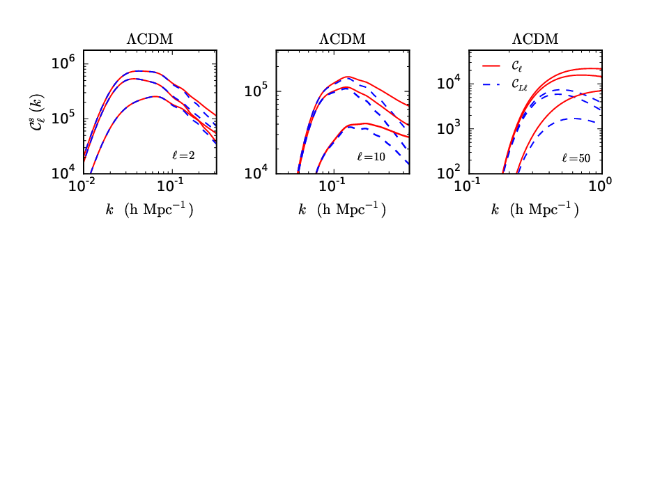
We show the diagonal entries of the 3D sFB power spectrum , as defined in Eq.(46), in Figure-4, for the CDM cosmology. We also plot separately the contributions (equal to the real-space power) and (the redshift space contribution at first order over the peculiar velocity power spectrum). In each case we also display the linear power spectra defined by Eq.(49).
We find that the non-linear contributions are quite small below Mpc-1 but cannot be neglected at higher . This transition scale also corresponds to the harmonic . For higher the non-linear contribution becomes more pronounced at lower . The redshift space distortions typically give a contribution to the total power on the scales displayed in Figure-4.
4.2 Off-diagonal terms of the power spectrum matrix
 |
 |
A few slices through the window functions and that represent mode-mixing in the presence of the radial selection function are displayed in Figure-5 for and Figure-6 for . For higher and the mode mixing is more suppressed, that is, the window function is more strongly peaked around .
 |
 |
The power spectra are diagonally dominated. However, a few off-diagonal terms of the matrix are displayed in Figure-7 (for ) and Figure-8 (for ). The left and right panels show and , respectively. For higher the covariance matrix is more sharply peaked at . The slices through the covariance matrix for as depicted in Figure-8 are more sharply peaked compared to the results for the same values of . These properties follow from the behaviour of the window functions displayed in Figure-5 and -6. To compare the diagonal elements with the off-diagonal terms we have also shown in these plots (dashed-lines).
4.3 Impact of the modified gravity models


In Figure-9 and Figure-10 we plot the diagonal entries of the 3D sFB power spectrum , as defined in Eq.(46), as a function of the wave number for gravity theories. The results correspond to and respectively. The range of -values probed is -. In Figure-9 we show the results for and in Figure-10 we show the results for . For each value of we show the three values . The base -CDM model is also plotted (solid lines). In comparison to the -CDM model all models have additional power at all . We find that for all values of and the redshift-space contribution is positive. We will see that the inclusion of redshift information improves our ability to distinguish departures of MG theories from GR.
 |


The Dilaton models we consider are specified by the four parameters , , and , as given in Table-1. The results for , and are presented in Figures-11, -12 and -13, respectively. In agreement with the 3D power spectra shown in Figure-3, over the range and associated with linear and weakly non-linear scales, the relative deviations from the CDM power grow at higher radial wave number and angular harmonic .
5 Covariance and
The likelihood function for arbitrary sets of parameter (that specify a given MG theory; e.g. in the case of theory), given the data vector (which consists of the noisy 3D sFB power-spectra ), is given by:
| (51) |
Here ( being the power spectrum in GR); is the size of the data vector, which depends on the angular resolution and the number of radial bins used in the computation. The covariance matrix is given by:
| (52) |
where we used a Gaussian approximation. Here represents the number density of galaxies which are assumed to be Poisson distributed. The block diagonal form is a result of assuming an all-sky coverage. However we found the to be diagonally dominant. Partial sky coverage will introduce off-diagonal terms between different harmonics in the covariance matrix. A rough scaling of signal-to-noise (S/N) with the fraction of sky-coverage is typically used in the literature: . We work with the statistics defined as:
| (53) |
We assume a perfect knowledge of all background cosmological parameters and present results with and without RSD. In practice, we bin the radial wave number in four logarithmic bins to avoid the covariance matrix being singular, thus replacing the integrals over and by discrete sums, and we use the multipoles to . The galaxy number density is fixed at . We again assume all-sky coverage and the survey depth is fixed at .

We show our results for the theories in Figure-14. For the model we find that for the values of can be ruled out with a confidence. For we find the constraint degrades to . The models with higher exponent are progressively less constrained as they converge increasingly fast to CDM with redshift at .

We show our results for the Dilaton models in Figure-15. We consider the problem of the estimation of each individual parameter while keeping others fixed, which corresponds to the model families A, B, C and E. For we find that the parameter values and can be ruled out with confidence. No meaningful constraints on or can be obtained at level. Clearly, a joint estimation will be more demanding. These parameters will also have some degeneracy with the parameters describing the background cosmological dynamics. A joint Fisher analysis of MG parameters and cosmological parameters will require a dedicated study and will be presented elsewhere. As the Planck observations provide an accurate baseline standard cosmological model, using Planck prior may be a useful practical solution.
The comparison of the linear and non-linear curves in Figures-14 and -15 suggests that the non-linear contributions can make a significant effect. However, in the non-linear regime the covariance matrix should include the bispectrum and the trispectrum of the density field, which would reduce the . Therefore, we can expect that a fully non-linear analysis, with a better modelling of the covariance matrix (e.g., from numerical simulations) would lower down the non-linear curves and make them closer to the linear result. However, because the departures from the CDM power spectrum increase on weakly non-linear scales, non-linearities should still improve the discriminatory power of the analysis of 3D clustering as compared with the linear result. Here we follow a conservative approach as we estimate the constraints on the modified-gravity parameters by using the linear-theory .
We have studied the constraints in both and Dilaton models with and without redshift space distortion. We find that redshift space distortions only lead to a small broadening of the constraints. Below galaxy number density of the surveys rapidly lose their ability to discriminate. On the other hand, increasing the number density beyond does not lead to drastic improvements of the results.
Our constraints are derived for a spectroscopic survey. Inclusion of photometric redshift error will degrade the discriminating power of the survey.
Our constraints are based on lower order tangential modes . We find that the information contents in different are highly degenerate. In the range , we find that for more than three to four (logarithmic) bins in the covariance matrix can become singular.
Finally, our results are based on an uniform distribution of noise (constant ) while real surveys may have more complicated variations in the average galaxy number density which may depend on the radial and angular coordinates in the sky.
6 Discussion & Future Prospects
In this paper we have studied the possibility of constraining modified gravity theories using galaxy clustering. We have studied two different modified gravity models: theories and Dilaton theories. In both cases we have used a specific parametrization and computed the as a criterion for constraining the departure from the CDM models. We used the sFB transforms and the resulting 3D power spectrum for a range of and values to constrain the model. We assume an all-sky coverage and a spectroscopic survey with a Gaussian selection function Mpc. We fix the number density of galaxies to be . We find that the low modes of (with radial modes restricted to ) can constraint the parameter at a level of with confidence for . For the Dilaton models some of the parameters () can be well constrained using galaxy clustering though there are others () which remain poorly constrained. The parametrization used by us depends on a tomographic approach. Combining constraints from higher modes can further reduce the error-bar and thus in principle make cosmological probes of gravity competitive with solar system tests. However this will require an accurate modelling of non-linear clustering in redshift space as well as the covariance matrix of the sFB power spectra. Our results are based on the linear power spectrum. However, we find that inclusion of nonlinear effect can drastically improve the . However we would like to emphasise that the contribution from higher order moments notably the trispectrum is not included in our covariance matrix. Although, this may not play an imprortant role in the quasi-linear regime, in the nonlinear regime such contributions can no longer be ignored. A detailed analysis will be presented elsewhere. Partial sky coverage, boundary conditions from specific survey geometry will also mean that in a realistic survey the sFB modes will have to be discrete and not continuous even in the radial direction. The average number density of galaxies and hence the noise too will be a function of the angular position on the surface of the sky. A pseudo- (PCL) based approach can be useful in this direction. The errors due to photometric redshift determination can be readily included in our calculation.
We have only considered two sets of MG theories. However, the results derived are quite general and can readily be extended to other MG scenarios such as the K-mouflage models or the Symmetron models. In addition, the sFB power spectrum can also be useful in constraining massive neutrinos, warm dark matter candidates or axionic dark matter through their footprints on the matter power spectrum as a function of redshift.
The number of parameters required to specify a MG model can be high. Non-parametric techniques such as Principal Component Analysis (PCA) can be efficient to investigate linear combinations (ordered according to decreasing signal-to-noise) of parameters that can be extracted using a specific survey strategy. Extending the based approach presented here, a more extensive analysis of survey optimisation covering a range of survey parameter and associated Fisher matrix analysis detailing parameter degeneracies will be presented elsewhere. In future we also plan to use a Bayesian model selection approach based on the evidences for acceptance or rejection of specific models.
Physics of galaxy formation may be different in modified gravity models. Even in the CDM cosmology, the bias associated with the galaxies may depend on the galaxy type and their environment, and may be stochastic. Such complications can only be dealt with numerical simulations. However, one may expect that at very large scale such effects may be less important.
CMB mostly probes high redshifts where any modification from GR is expected to be sub-dominant. However, CMB is also sensitive to modifications of gravity through secondary effects such as the Integrated Sachs-Wolfe (ISW) effect and the weak lensing distortions (Planck Collaboration, 2015a). However the constraints are rather weak compared to what can be achieved by galaxy surveys (Munshi et al., 2014).
Weak lensing is a very exciting possibility for constraining any departure from GR especially because it is free from the problem of galaxy bias (Munshi et al., 2008). However, in recent years many possible systematics have been discussed, e.g. from intrinsic ellipticity correlations or possible modifications of the power spectrum due to AGN feedback, gas cooling and stellar feedback or neutrino physics (Munshi et al. 2015; in preparation). Such contaminations may induce appreciable bias in parameter estimation (e.g. (Osato, Shirasaki, & Yoshida, 2015)). Despite all these systematics, weak lensing and galaxy clustering remain the most powerful probe of possible departures from GR on cosmological scales.
Statistics of Lyman- absorbtion have also been investigated in the context of gravity (Arnold, Puchwein & Springel, 2015). Using cosmological hydrodynamical simulations of gravity which include the flux probability distribution functions and the flux power-spectra, and an analysis of the column density and line-width distributions, as well as the matter power spectrum, It was found that Lyman- statistics is rather insensitive to modification to gravity in models. Hence no competitive constraints are achievable using current data. Moreover, contamination by baryonic physics, associated with star formation and cooling processes, imply that a very accurate modelling of such ingredients is required. Constraints from cm intensity mapping are more encouraging (Hall et al., 2013).
Observations by SDSS galaxy surveys in the low to moderate redshift range is already being used to set interesting constraints on any departure from GR, e.g. Bel et al. (2014) obtained at the confidence level. Euclid with survey characteristics similar to SDSS will probe deeper and wider parts of the sky thus improving the constraints by orders of magnitude.
Acknowledgements
D.M. and P.C. acknowledge support from the Science and Technology Facilities Council (grant number ST/L000652/1). The research leading to these results has received funding from the European Research Council under the European Union’s Seventh Framework Programme (FP/2007-2013) / ERC Grant Agreement No. [616170]. P.V. acknowledges support from the French Agence Nationale de la Recherche under Grant ANR-12-BS05-0002. D.M. would like to thank A. Starobinsky and A. Heavens for useful discussions. It is a pleasure for D.M. to acknowledge related collaborations with B. Hu, L. van Waerbeke and J. Harnois-Deraps.
References
- Abramo et al. (2010) Abramo L.R., Reimberg P.H., Xavier H.S., 2010, PRD, 82, 043510
- Alcock & Paczynski (1979) Alcock C., Paczynski B., 1979, Nature, 281, 358
- Allemandi, Borowiec & Francaviglia (2004) Allemandi G., Borowiec A., Francaviglia M., 2004, PRD, 70, 103503
- Amendola, Kunz & Sapone (2008) Amendola L., Kunz M., Sapone D., 2008, JCAP, 4, 13
- Amendola et al. (2011) Amendola, L. et al., 2011, JCAP, 1107, 027
- Arnold, Puchwein & Springel (2015) Arnold C., Puchwein E., Springel V., 2015, MNRAS, 448, 2275
- Asrorey et al. (2012) Asorey J., Crocce M., Gaztanaga E., Lewis A., 2012, MNRAS, 427, 1891
- Bel et al. (2014) Bel J., Brax P., Marinoni C., Valageas P., 2014, arXiv:1406.3347
- Bertschinger (2006) Bertschinger E., 2006, ApJ., 648, 797
- Bernardeau et al. (2002) Bernardeau F., Colombi S., Gaztanaga E., Scoccimarro R., 2002, Phys.Rept, 367, 1, 248
- Brax, Davis & Li (2012) Brax P., Davis A.-C., Li B., 2012, PhLB, 715, 38B
- Brax et al. (2012) Brax P., Davis A.-C., Li B., Winther H. A., Zhao G.-B., 2012, JCAP 10, 002
- Brax et al. (2012) Brax P., Davis A.-C., Li B., Winther H. A., 2012, PRD, 86, 044015
- Brax & Valageas (2013) Brax P., Valageas P., 2013, PRD, 88, 023527
- Brax et al. (2004) Brax P., van de Bruck C., Davis A.-C., Khoury J., Weltman A., 2004, PRD, 70, 123518
- Brax et al. (2008) Brax P., van de Bruck C., Davis A.-C., Shaw D.J., 2008, PRD, 78, 104021
- Buchdahl (1970) Buchdahl, H. A., 1970, MNRAS, 150, 1
- Castro, Heavens & Kitching (2005) Castro P.G., Heavens A.F., Kitching T.D., 2005, PRD, 72, 023516
- Cheung et al. (2008) Cheung, C., Fitzpatrick, A. L., Kaplan, J., Senatore, L., Creminelli, P., 2008, JHEP, 3, 14
- Chiba (2003) Chiba T., 2003, Phys.Lett. B575, 1
- Clifton et al. (2013) Clifton T., Ferreira P.G., Padilla A., Skordis C., 2012, Physics Reports 513, 1, 1
- Daniel et al. (2010) Daniel, S.F., et al. 2010, PRD, 81, 123508
- Damour & Polyakov (1994) Damour T. & Polyakov A.M., 1994, Nucl. Phys. B423, 532
- Dosset, Hu & Parinson (2014) Dosset J., Hu B., Parkinson D., 2014, JCAP, 1403, 046
- Erdogue et al. (2006) Erdogue P. et al., 2006, MNRAS, 368, 1515
- Ferreira & Skordis (2010) Ferreira P.G., Skordisn C., 2010, PRD, 81, 104020
- Fisher et al (1995) Fisher K.B., Lahav O., Hoffman Y., Lynden-Bell D., Zaroubi S., 1995, MNRAS, 272, 885
- Gil-Marin et al. (2011) Gil-Marin H., Schmidt F., Hu W., Jimenez R., Verde L., 2011, JCAP, 1111, 019
- Guzzo et al. (2008) Guzzo L., et al., 2008, Nature, 451, 541
- Hall et al. (2013) Hall A., Bonvin C., Challinor A., 2013, PRD, 87, 064026
- Heavens (2003) Heavens A., 2003, MNRAS, 343, 1327
- Heavens, Kitching & Verde (2007) Heavens A.F., Kitching T.D., Verde L. 2007, MNRAS, 380, 1029
- Heavens & Taylor (1995) Heavens A., Taylor A., 1995, MNRAS, 343, 1327
- Hinterbichler & Khoury (2010) Hinterbichler K., Khoury J., 2010, PRL, 104, 231301
- Hivon et al. (2002) Hivon E., Górski K. M., Netterfield C. B., Crill B. P., Prunet S., 2002, ApJ, 567, 2
- Hojjati (2011) Hojjati A., Zhao G.B., Pogosian L., Silvestri A., Crittenden R., Koyama K., 2012, PRD, 85, 043508
- Hu & Sawicki (2007) Hu W., Sawicki I., 2007, PRD, 76, 06004
- Hu & Sawicki (2007) Hu W., Sawicki I., 2007, PRD, 76, 104043
- Jackson (1972) Jackson J. C., 1972, MNRAS, 156, 1P
- Jain, Vikram & Sakestein (2013) Jain B., Vikram V., Sakstein J., ApJ, 2013, 779, 39
- Jain & Zhang (2008) Jain B. & Zhang P., 2008, PRD, 78, 063503
- Jennings et al. (2012) Jennings E., Baugh C.M., Li B., Zhao G.B. & KoyamaK., 2012, MNRAS, 425, 2128
- Joyce et al. (2014) Joyce A., Jain B., Khoury J., Trodden M., 2015, Physics Reports, 568, 1
- Kaiser (1987) Kaiser N., 1987, MNRAS, 227, 1
- Laureijs (2011) Laureijs R. et al. arXiv:1110.3193
- Lanuss, Rassat & Strack (2012) Lanusse F., Rassat A., Starck J.-L., 2012, A&A, 540, 60
- Li et al. (2000) Li B., Hellwing W.A., Koyama K., Zhao G.B., Jennings E., Baugh C.M., 2013, MNRAS, 428, 743
- Li, Mota & Barrow (2011) Li B., Mota D.F., Barrow J.D., 2011, ApJ, 728, 109
- Linder (2005) Linder E.V.,2005, PRD.,72, 043529
- Lombriser et al. (2012) Lombriser L., Slosar A., Seljak U., Hu W., 2012, PRD, 85, 124038
- Munshi, Heavens & Coles (2011a) Munshi D., Heavens A., Coles P., 2011a, MNRAS, 411, 2161
- Munshi et al. (2014) Munshi B., Hu B., Renzi A., Heavens A., Coles P., 2014, MNRAS, 442, 821
- Munshi et al. (2011b) Munshi D., Kitching T., Heavens A., Coles P., 2011b, MNRAS, 416, 629
- Munshi et al. (2008) Munshi, D., Valageas, P., van Waerbeke, L., Heavens, A., 2008, PhR, 462, 67M
- Navarro, Frenk & White (1996) Navarro J.F., Frenk C.S., White S.D.M., 1996, ApJ., 462, 563
- Nunez & Solgnaik (2004) Nunez A., Solganik S., arXiv:hep-th/0403159
- Olive & Pospelov (2008) Olive K.A., Pospelov M. Phys 2008, PRD, 77, 043524
- Osato, Shirasaki, & Yoshida (2015) Osato, Ken; Shirasaki, Masato; Yoshida, Naoki, 2015, ApJ, 806, 186
- Ostriker & Steinhardt (2003) Ostriker J.P., Steinhardt P., 2003, Science, 300, 1909
- Oyazu, Lima & Hu (2008) Oyaizu H., Lima M., Hu W., 2008, PRD, 78, 123524
- Perlmutter et al. (1999) Perlmutter S. et al., 1999, ApJ, 517, 565
- Pietroni (2005) Pietroni M., 2005, PRD, 72, 043535
- Planck Collaboration (2015a) Planck Collaboration, 2015, arXiv:1502.01590
- Pogosian & Silvestri (2008) Pogosian L., Silvestri A., 2008, PRD, 77, 023503
- Pratten & Munshi (2014) Pratten G., Munshi D., 2014, MNRAS, 442, 759
- Pratten & Munshi (2013) Pratten G., Munshi D., 2013, MNRAS, 436, 3792
- Rassat et al. (2005) Rassat A. et al. 2005, astro-ph/0510195
- Rassat & Refregier (2012) Rassat A., Refregier A., 2012, A&A, 540, 115
- Ries et al. (1998) Riess A. G. et al., 1998, Astron J., 116, 1009
- Schimdt (2008) Schimdt F., 2008, PRD., 78, 3002
- Schlegel et al. (2007) Schlegel D.J. in Bulletin of the American Astronomical Society Meeting Abstracts, volume 211, 132.29
- Shapiro, Crittenden, Percival (2011) Shapiro C., Crittenden R.G., Percival W.J., 2012, MNRAS, 422, 2341
- Song, Hu & Sawicki (2007) Song Y.-S., Hu W., Sawicki I., 2007, PRD, 75, 044004
- Song, Peiris & Hu (2007) Song Y.-S., Peiris H., Hu W., 2007, PRD, 76, 063517
- Starobinsky (1980) Starobinsky, A. A., 1980, Physics Letters B, 91, 99
- Starobinsky (2007) Starobinsky, A. A., 2007, JETPL, 86, 157
- Tsujikawa & Tatekawa (2008) Tsujikawa S., Tatekawa T. 2008, Phys.Lett. B, 665, 325
- Tyson & LSST (2004) Tyson J.A. & LSST in Bulletin of the American Astronomical Society Meeting Abstracts, volume 36 108.01
- Vainshtein (1972) Vainshtein A., 1972, Phys.Lett. B39, 393
- Valageas (2013) Valageas P., 2013, Phys. Rev. D 88, 083524
- Valageas, Nishimichi & Taruya (2013) Valageas P., Nishimichi T., Taruya A., 2013, Phys. Rev. D 87, 083522
- Vikram et al. (2013) Vikram V., Cabre A., Jain B., VanderPlas J.T., 2013, JCAP, 1308, 020
- Zhang (2006) Zhang P., 2006, PRD, 73, 123504
- Zhao et al. (2010) Zhao G.B., Giannantonio T., Pogosian L., Silvestri A., Bacon D.J., Koyama K., Nichol R.C., Song Y.S., 2010, PRD, 81, 103510
- Zhao (2010) Zhao G.B., Li B. & Koyama K., 2011, PRD, 83, 044007
- Zhang et al. (2007) Zhang P., Liguori M., Bean R., Dodelson S., 2007, PRL, 99, 141302
- Zhao et al. (2009) Zhao G.B., Pogosian L., Silvestri A., Zylberberg J., 2009, PRL, 103, 241301
- Zhao et al. (2008) Zhao G.B., Pogosian L., Silvestri A., Zylberberg J., 2008, PRD, 79, 083513