Trojan dynamics well approximated
by a new Hamiltonian
normal formThanks: Key words and phrases: Restricted
three-body problem, normal forms, Hamiltonian perturbation theory,
averaging, Celestial Mechanics
Abstract
We revisit a classical perturbative approach to the Hamiltonian related to the motions of Trojan bodies, in the framework of the Planar Circular Restricted Three-Body Problem (PCRTBP), by introducing a number of key new ideas in the formulation. In some sense, we adapt the approach of [11] to the context of the normal form theory and its modern techniques. First, we make use of Delaunay variables for a physically accurate representation of the system. Therefore, we introduce a novel manipulation of the variables so as to respect the natural behavior of the model. We develop a normalization procedure over the fast angle which exploits the fact that singularities in this model are essentially related to the slow angle. Thus, we produce a new normal form, i.e. an integrable approximation to the Hamiltonian. We emphasize some practical examples of the applicability of our normalizing scheme, e.g. the estimation of the stable libration region. Finally, we compare the level curves produced by our normal form with surfaces of section provided by the integration of the non–normalized Hamiltonian, with very good agreement. Further precision tests are also provided. In addition, we give a step-by-step description of the algorithm, allowing for extensions to more complicated models.
1 Introduction
Series expansions in terms of small physical parameters are a common way of dealing with dynamical models in Celestial Mechanics. One case where this approach has been extensively used is the problem of Trojan motion. The so-called Trojan stability problem, i.e. the study of the long-term dynamics for massless particles in the neighborhood of the equilateral Lagrangian points, has been studied both analytically and numerically in several contexts11 1 For an introduction to Trojan dynamics, see, e.g., [9].
From the numerical point of view, quite complete models (including extra planets perturbations and/or 3-dimensional configurations) are possible to consider. Such experiments are in general based on accurate long integrations, done through high precision integrators. A clear outcome is the determination of size and shape of the stable domain around the equilibrium points. Secondary resonances embedded within the domain of the 1:1 Mean Motion Resonance (MMR) are of particular importance in the stability issue. For example, in [22] and [23], the importance of the resonance web is highlighted for what concerns the process of de-population of the Trojan domain, in the case of Jupiter’s asteroids. In [6], the authors study the orbital stability of the only discovered Trojan asteroid of the Earth, i.e. 2010 TK7, and determine the stability region around L4 and L5 in the Sun-Earth system.
Besides pure numerical investigations, several works have also explored the applicability of analytical methods in the problem of Trojan stability. In particular, the Trojan problem has served as a classical model for testing methods based on the construction of a so-called Hamiltonian normal form approach.
Semi-analytic methods share a common structure: each method is based on an explicit algorithm, possible, as a rule, to translate into a programming code, which computes the expansion of a suitable normal form that provides some special solutions. Therefore, a normal form is a good local approximation to the complete Hamiltonian, used to reproduce the orbits of particular objects.
Normal forms have been used in several cases for computing the size and shape of the stability domain. From the point of view of Nekhoroshev stability estimates [18],[19], examples of this computation are in [4], [13], [8], [16], [7]. On the other hand, in [10], the stability estimation is induced by applying the Kolmogorov-Arnold-Moser (KAM) theory. But all these approaches, while introducing novel and promising features, tend to fail when it comes to reproduce the numerical results about the size and shape of the whole stability region. In general, they are able to justify stability for just a small subset of Trojan orbits, located relatively close to the equilibrium point.
In the present work, we develop a new normal form approach to the classical PCRTBP by combining three main ideas. First, we make an accurate choice of variables for the representation of the system. Second, we explicitly take benefit of the existence of a slow and a fast degree of freedom, dealing with them differently in our normal form construction. Finally, we make use of Lie series techniques for the averaging over the fast angle; in fact, as shown below, a key element of our method is that such a treatment makes possible to overcome the only true singularity that the Trojan motion contains, namely the eventual close encounters with the primary.
We motivate these ideas as follows.
Many of previous attemps describe the system in terms of cartesian coordinates, which however do not capture properly the physical configuration of the model. Considering canonical variables well adapted to the system helps to improve the accuracy of the normal form and the estimation of stability domains. To this end, in the present paper, we adopt (and show the usefulness of) a modified version of Delaunay-like coordinates introduced long ago in [11].
Regarding the other two ideas, an important point is that the only real physical singularity in the 1:1 MMR region is due to possible collisions / close encounters of the Trojan body with the primary. In our setting of modified Delaunay-like variables (see definition 4), this singularity takes place at , where is the synodic mean longitude of the massless body. Thus, any polynomial expansion around the equilibrium point, exhibits a bad convergence behavior for orbits approaching this singularity. Nevertheless, in this work we show this problem can be overcome in a rather simple way. This is based on the following remarks.
On one hand, as noted already, an inspection of the main terms of the Hamiltonian for a Trojan body, indicates that the motion is ruled by a fast and a slow frenquency. In Delaunay variables, these two dynamics are represented by two independent pairs of canonical coordinates. However, the long term behavior of the orbits depends essentially only on the slow degree of freedom which, in our variables, corresponds to the canonical pair including the angle . In other words, an appropriate normal form construction that aims to study the long term dynamics involves averaging over the fast angle only. This produces an integrable Hamiltonian of two degrees of freedom in which the fast angle is ignorable.
On the other hand, such an averaging implies that one has to solve a so-called homological equation in which plays no role. As shown in Section 2 below, due to this property, one can retain in the Hamiltonian a complicated functional dependence on , other than trigonometric or simply polynomial. In our case this dependence turns to be of the form of powers of the quantity . Thus, using this technique allows to greatly extend the convergence domain of the final normal form.
Finally, we develop a new normalization algorithm for the computation of the integrable approximation, by using the Lie series formalism, adapting to a modern way the technique described in [11]. With this integrable normal form, we can approximate Trojan orbits having either tadpole or horseshoe shapes, even in cases where distances from the equilateral point become large and where previous approaches tend to fail.
There are several different examples where such a normalizing scheme can be applied. The most evident corresponds to the use of the scheme for the estimation of the stability domain. Such a computation, in the same direction as the references mentioned before, aim to estimate the effects induced by the remainder (in later Eq. 11) of the normal form produced by the algorithm. According to our results, our novel normalization may radically improve the results regarding the size of the domain of stability around the equilateral Lagrangian points, understimated so far. Other examples inherent directly to the normal form can be mentioned. For instance, in [21], we used the normalized coordinates for the design and optimization of maneuvers aiming to transfer a spacecraft into the tadpole region. Moreover, the numerical experiments described in the present work highlight that our method allows to clearly differentiate the tadpole region from the horseshoe region. In some cases, when the mass ratio between the two primary bodies is very small and consequently also the chaotic regions are small, such a computation gives a first order estimation of the stable tadpole domain. On the other hand, this kind of perturbative approach is motivating for problems of diverse nature. For instance, in [3], they make use of the Relegation algorithm, that shares a similar structure with our normalizing scheme, to compute some particular orbits around an irregularly shaped asteroid.
This paper is structured as follows: in Section 2, we describe the expansion and normalization scheme, applied to the case of the PCRTBP Hamiltonian, in the 1:1 MMR region; in Section 3, we provide different tests for a suitable accuracy verification of the normal form, involving comparisons with the numerical integration of the full problem; in Section 4, we summarize the work and outline future applications of this method. Furthermore, Appendix A formally presents the algorithm in such a way that it can be adapted also to different models, for example, the Elliptic Restricted Three Body Problem (ERTBP) or the Restricted MultiPlanet Problem (RMPP), described in [20].
2 Construction of the integrable approximation
2.1 Initial settings
In heliocentric canonical variables , the Hamiltonian of the PCRTBP can be written as:
| (1) |
where and are the masses of the larger and smaller primary, respectively, is the heliocentric position vector of the test particle, the one corresponding to the second primary, , , and .
In what follows, , , and symbolize the major semi-axis, the eccentricity, the mean anomaly and the longitude of the perihelion (primed quantities correspond to the primary). We set the unit of length as , and the unit of time such that the mean motion of the primary is equal to . This implies . The unit of mass is set so as to . Defining the mass parameter as , the Hamiltonian in the above units takes the form:
| (2) |
where the so–called disturbing function is such that
| (3) |
Including the small keplerian correction in the disturbing function allows to define action-angle variables with values independent of the mass parameter . Inspired by [20] and references therein, we introduce modified Delaunay action-angle variables
|
|
(4) |
According to the definitions of the orbital elements above, is the synodic mean longitude. In order to remove the fictitious singularity of the Delaunay–like variables when (i.e., for circular orbits), it is convenient to introduce canonical coordinates , similar to Poincaré coordinates for the planar Keplerian problem. Thus, let us define
|
|
(5) |
where the values of , and are significantly small in a region surrounding the triangular Lagrangian points, for instance, in the case of tadpole or horseshoe orbits (since and ). Let us recall that those variables have been introduced in [11] to study the PCRTBP.
Before starting the construction of the normal form, it is necessary to express Hamiltonian (2), in particular the disturbing function in (3), in terms of Poincaré–Delaunay–like coordinates . Here, we limit ourselves to sketch this preliminary procedure22 2 An exhaustive description of those expansions is out of the scopes of this publication. All the details are deferred to Páez, R.I., Ph.D. Thesis (2015), that is in preparation and is available on request to the author.. Essentially, as a first step, the terms , and (appearing in the Hamiltonian) must be expanded with respect to orbital elements , , and , following e.g. §6 in [17]. Afterwards, the eccentricity is replaced by its expansion in power series of the parameter . By using the equations , , , we can then express , and as functions of the canonical variables (5).
As explained in the Introduction, the particular normalizing scheme we use allows to keep a non polynomial nor trigonometric functional dependence with . By making use of this idea, we keep powers of , in the expansions of the term of , which describes the main part of the inverse of the distance from the primary (for values of the major semi-axis and small eccentricity). Thus, the Hamiltonian ruling the motion of the third body takes the following form 33 3 The first term in (6) comes from the expansion of the Keplerian part, i.e. the part of the Hamiltonian independent of , in terms of , and , that corresponds to .
|
|
(6) |
where are rational numbers. Actually, we just produce a truncated expansion of formula (6) up to a finite polynomial degree in , and , by using Mathematica. By inspection, we check that both properties and are satisfied in our initial expansion, and we just conjecture that they hold true also to any following polynomial degree in , and (being such a proof beyond of the scopes of this work).
2.2 Algorithm constructing the normal form averaged over the fast angle
Let us focus on the first main terms of the Keplerian part:
| (7) |
where we refer to the dynamics of the new canonical coordinates by retaining the old action–angle pair , that allow us to sketch our strategy in a simpler way. Indeed, the previous formula shows that the angular velocities have different order of magnitude
| (8) |
because and the values of the actions and are small in a region surrounding the Lagrangian points. Thus, can be seen as a slow angle and as a fast angle. This motivates to average the Hamiltonian over the fast angle (see, e.g.,§ 52 of [2]), in order to focus mainly on the secular evolution of the system. Therefore, we want remove (most of) the terms depending on the fast angle , that can be conveniently done in the setting of the variables , by performing a sequence of canonical transformations. In the following, this strategy is translated in an explicit algorithm using Lie series, by adapting to the present context an approach that has been fruitfully applied to various problems in Celestial Mechanics (for instance, for locating the elliptic lower-dimensional tori in a rather realistic four-body planetary model in [24], or studying the secular behavior of the orbital elements of extrasolar planets in [15]). By applying such a procedure to our Hamiltonian model, we construct an average normal form, satisfying two important properties: (I) it provides an accurate approximation of the starting model; (II) it only depends on the actions and one of the angles and, therefore, it is integrable.
Our final normal form is produced by an algorithm dealing with a sequence of Hamiltonians, whose the expansion can be conveniently described after introducing the following
Definition 2.1
A generic function belongs to the class , if its expansion is of the type:
where are real coefficients.
Let and be two integer counters, running in the intervals and , respectively, being fixed numbers. At each –th step, our algorithm introduces a new Hamiltonian such that
|
|
(9) |
where , , , , and . From (9), we emphasize that
- •
The splitting of the Hamiltonian in sub-functions belonging to different sets basically gather all the terms with the same order of magnitude and total degree (that can be semi-odd) in the actions and . This is made in order to develop a normalization procedure, exploiting the existence of natural small parameters: and the values of the pair of actions .
- •
- •
Our algorithm requires just normalization steps, which are performed by constructing the finite sequence of Hamiltonians
They are defined so that and the –th normalization step is performed by a canonical transformation. This recursively introduces the new Hamiltonian in such a way that
| (10) |
with a generating function that is determined by solving a so–called “homological equation”, while denotes nothing but the Lie series operator. The Lie derivative is such that is the classical Poisson bracket, with a generic function defined on the phase space and any generating function (see, e.g., [12] for an introduction to canonical transformations expressed by Lie series in the context of the Hamiltonian perturbation theory). All the recursive formulas, which determine the terms of type and appearing in (9), are reported in Appendix A. Let us stress that, after each transformation, in the present subsection we do not change the name of the canonical variables in order to simplify the notation. We emphasize here that the new generating function introduced at the generic –th step, namely , is determined so as to remove from the main perturbing term44 4 Let us recall that the size of is expected to decrease when the indexes or are increased, because the values of , and are assumed to be small its subpart that is not in normal form.
We rewrite the final Hamiltonian in such a way to distinguish the normal form part from the rest, as follows:
| (11) |
where all the averaged terms of type are gathered into the integrable part , while the others contribute to the remainder . Here, our algorithm is described at a purely formal level in the sense that the problem of the analytic convergence of the series on some domains is not considered. However, it is natural to expect that our procedure defines diverging series into the limit of , because a non-integrable Hamiltonian cannot be transformed in an integrable one, on any open domain. In principle, the values of both integer parameters and should be carefully chosen in such a way to reduce the size of as much as possible. In practice, we simply fixed the values of and according to the computational resources, in order to deal with the application described in the following section 3.
2.3 Numerical computation of the flow induced by the integrable approximation
Lie series induce canonical transformations in a Hamiltonian framework; this fundamental feature allows us to design a numerical integration method, by using both the normal form previously discussed and the corresponding canonical coordinates. Let us denote with the set of canonical coordinates related to the –th normalization step. By applying the so–called ’exchange theorem’ (see [12]), we have that
| (12) |
where the variables related to the previous step, i.e. , are given as
| (13) |
According to this, Lie series must be applied separatedly to each variable, in order to properly define all the coordinates for the canonical transformation . Thus, the whole normalization procedure is described by the canonical transformation
| (14) |
Such a composition of all the intermediate changes of variables can be used for providing the following semi-analytical scheme to integrate the equations of motion:
| (15) |
where denotes the flow induced on the canonical coordinates by the generic Hamiltonian for an interval of time equal to . Let us emphasize that the above integration scheme provides just an approximate solution. From an ideal point of view (i.e., if all the expansions were performed without errors and truncations), formula (15) would be exact if the normal form part would correspond to the complete Hamiltonian ; moreover, is integrable and its flow is easy to compute55 5 In order to explicitly describe the solutions of the equation of motions for the normal form , it is convenient to introduce the temporary action–angle variables such that and , where is a constant of motion for the normal form . By considering as a fixed parameter and using the standard quadrature method for conservative systems with d.o.f., one can compute and at any time . The same can be done for the evolution of , by evaluating the integral corresponding to the differential equation . For practical purposes, the application of the classical quadrature method can be replaced by any numerical integrator that is precise enough. Finally, the values of and can be directly calculated from those of the corresponding action–angle variables, that are and ., reasons why using becomes valuable. According to equation (11), the approximate solution provided by the scheme (15) is as more accurate as smaller the perturbing part is with respect to .
A key point concerns the structure of our expansions. If we truncate the r.h.s. of equation (9) up to a finite order of magnitude in and a fixed total degree in the actions and , since each term of type and is included in a corresponding class of functions , the truncated expansion of just include a finite number of monomials. The same applies also to the truncated expansions of both the final Hamiltonian and the canonical transformation . Therefore, after introducing the truncation rules, the normalization algorithm require a finite total number of operations, to compute the elements necessary to implement the whole integration scheme (15). Thus, it can be translated in a programming code.
In order to concretely apply our semi-analytical scheme, by using Mathematica, we compute the truncations up to the terms and to the fifth total degree with respect to the square roots of the actions and (i.e. , , in order to obtain , and its inverse). At the end of its execution, that code writes, on an external file, C functions which are able to compute the changes of coordinates induced by and by its inverse. Moreover, it provides also another external file, where the integrable equations of motion related to the Hamiltonian are written according to the syntax of the Taylor66 6 Taylor is an automatic translator producing a C function acting as a time-stepper specific for a given ordinary differential equation (by means of the Taylor method). It is publicly available at the following website: http://www.maia.ub.es/angel/soft.html software package. A basic use of the Linux shell scripting allowed us to automatically complement all these parts of the computational procedure, so as to produce a new C program as an output. This final code is able to numerically integrate the equations of motion via the scheme (15), where the flow is computed by using the Taylor method (based on the automatic differentiation technique, see [14] and [1]). The truncation rules are fixed in such a way to execute all the computations in a reasonable amount of CPU-time.
3 Accuracy control for the normal form
An averaged model approximating a certain problem is powerful to the extent that it reproduces the main features of the original system, (in this case the Planar Circular Restricted Three Body problem). It is widely proved that PCRTBP is barely a very simplistic representation for the Trojan motion, but its basic dynamics allows us to test in a simple way the normalization method. Furthermore, according to the nature of the method, much more complex (i.e., non-planar, eccentric, including additional planets) models can be treated without any substantial change in the averaging scheme.
When seen from the most commonly used reference system (i.e. a synodic rotating frame with origin in the barycenter), motions around the equilateral Lagrangian points are represented by the so-called tadpole or horseshoe orbits (see §3.9 of [17]). In our set of variables, these orbits are characterized by large variations of the angle . So, as starting, a suitable averaged approximation has to be able to reproduce these variations correctly. In particular, this should apply even for the challenging case of bodies whose orbits lay very close to the border of the stability domain. As second goal, the averaged Hamiltonian should be able also to distinguish between tadpole orbits (around just one equilateral equilibrium point) and horseshoe orbits (around both points). In Section 2, we have provided an integrable averaged Hamiltonian (see 11), that explicitly describes the behavior of the degree of freedom related to the canonical pair of variables (,). In order to compare the original problem with our averaged version, we develop two different tests.
3.1 Numerical surfaces of section vs. semi-analytical level curves
The first test consists of a graphical comparison between the orbits provided by the complete Hamiltonian and those provided by normal form . In both cases, the initial conditions are fictitious, but each set is derived from the catalogued position of a real generating Trojan body. Since we are just interested in the behavior of the slow degree of freedom, for the complete problem (originally 4D), we just retain the evolution of the variables and by means of isoenergetic surfaces of section, which gives a 2D representation. In the two cases presented below, the generating bodies are 2010 TK7, Trojan asteroid of the Sun-Earth system and the asteroid 1872 Helenos of the Sun-Jupiter system.
From a catalogue, we obtain the coordinates (rotated to the plane of primaries) of each generating body for a certain epoch and we convert them to our canonical coordinates . This initial condition provides the Jacobi constant for the body, after which it is possible to produce an isoenergetic surface of section. We generate a set of 10 new orbits by keeping fixed the initial values for the variables and , scanning a range of values for and obtaining in such a way that (isoenergetic orbits). These initial conditions are numerically integrated for a short time, up to the variables accomplish the relation , where corresponds to the mean anomaly. We call this new set , and it generates both the surface of section and the level curves.
3.1.1 Computation of surfaces of section
Starting from Newtonian formulation for the PCRTBP, we derive the equations of motion for the third body in cartesian coordinates in the heliocentric system77 7 Although cartesian coordinates are not canonical conjugated variables, they provided the simplest closed form for these equations of motion, and for this reason they are still widely used for numerical experiments.
|
|
(16) |
where , , , correspond to cartesian positions and velocities of the massless body, and , give the instantaneous position of the planet. We translate initial conditions of the set to cartesian coordinates and we integrate them with a Runge-Kutta - order integrator, along 1500 periods of primaries, with time-step equal to . During this integration we collect the points contained in the pericentric surface of section, which in our case is represented by the condition
| (17) |
and provide about 1500 points per orbit. The output data is again translated to Delaunay variables and suitable to be compared with the results of the averaged Hamiltonian.
3.1.2 Computation of level curves
Through Hamilton’s equations, we can easily derive the equations of motion for the canonical variables and ,
| (18) |
Since is given by a series expansion of the variables , , , , and the small parameter , the equations of motion inherit the same structure. Through a suitable storing of the coefficients of these series and management of the equations of motion implemented in Mathematica (as explained in last paragraph of Subsection 2.3), we compute the evolution of the orbits according to the averaged Hamiltonian. Every initial condition of the set is first converted to normalized variables and then integrated up to collecting about 2000 points, keeping the relative energy error of the integration smaller than . Such a numerical integration is an efficient way to compute the level curves for the integrable normal form corresponding to the values and (in normalized variables).
We complement every point of a level curve with the values and (equivalent to ). Let us note here that the condition in the normalized coordinates does not correspond exactly to the surface of section in the original variables. However, since the change of coordinates (that gives the values of the non–normalized variables in the scheme (15)) is, by construction, a near-to-identity canonical transformation, we assume that the conditions for each surface of section do not differ too much. Finally, via , we back-transform all the points of a level curve in the original variables and we graphically compare them with the corresponding numerical surface of section.
3.1.3 Examples and results


We choose two systems with very different values of the mass parameter for a better contrast in the results of the test. The first case is provided by the PCRTBP approach to the Sun-Earth system, which is defined by a mass parameter . The generating body chosen for this system is the Earth only Trojan 2010 TK7, for which we obtain its coordinates from Jet Propulsion Laboratories JPL Ephemerides Service88 8 http://ssd.jpl.nasa.gov/?ephemerides, at epoch 2456987.5 JD (2014-Nov-26). We translate them to our set of canonical variables, resulting , , and . For the second case, we choose the Sun-Jupiter system, defined by the mass parameter . The generating body in this case is the Trojan asteroid 1872 Helenos, which belongs to the Trojan camp around L5 in such a system. The set of initial conditions for Helenos were obtained from Bowell Catalogue99 9 http://www.naic.edu/nolan/astorb.html, at 2452600.5 JD (2002-Oct-22), and after being translated to canonical Delaunay variables, they read , , and .
Figure 1 shows the comparison between the surface of section and the level curves computed for Sun-Earth system (left panel), and Sun-Jupiter system (right panel). For both cases, the points of the surface of section are represented in blue (dark gray) and the curves produced with the averaged Hamiltonian are in red (light gray). For the case of Sun-Earth system the agreement between the two representations is excellent. According to the milestones we define at the beginning of this section, the averaged Hamiltonian reproduces accurately the large variations of . In particular, it is perfectly able to distinguish between orbits belonging to the tadpole or to the horseshoe region. In the case Sun-Jupiter system, for which the mass parameter value is 3 orders of magnitude larger, there is a substantial presence of chaos. Nevertheless, the averaged Hamiltonian is able to locate any tadpole orbit provided by the complete Hamiltonian, even in cases when the motion is trapped into secondary resonances, and its validity is also good for orbits close to the border of the stable region.
3.2 Computation of quasi-actions
So far in the literature, one the most successful attemps to construct a normal form for testing the stability of Trojans in the context of the Hamiltonian formalism is discussed in [10]. However, of the 34 initial conditions they used for the system Sun-Jupiter, 4 presented orbits that were highly chaotic after being translated according their rotations into the planar CRTBP, while the Kolmogorov normalization algorithm defined in that work did not work properly for other 7 cases. Here, we revisit the fictitious initial conditions they considered for these latter seven asteroids (1868 Thersites, 1872 Helenos, 2146 Stentor, 2207 Antenor, 2363 Cebriones, 2674 Pandarus and 2759 Idomeneus). Since they conform a set of coordinates that either lay very close to the border of stability or show an anomalous behavior (with respect to the expected tadpole orbit), they provide a natural harder test in a more quantitative way.
In the previous subsection, we show that the evolution of the orbits given by emulates correctly in many cases the evolution under the original non-normalized Hamiltonian, by means of graphical comparisons between level curves and surfaces of section. This normal form contains two different actions or integrals of motion. One, obtained by construction and through the normalization, is given by . The other one, not explicitly obtained, is due to the fact that, after the reduction of , the normal form bear just 1 d.o.f., i.e. it is integrable. This second constant of motion is associated with the area enclosed by the level curve computed under the integration of , and therefore, provide another quantity to be checked. In order to do so, the computation of the orbits is done as explained in subsections 3.1.1–3.1.3, but for just one initial condition. After integrating both curves, we compute the maximum and minimum values for the two variables and reached during the integration. In Fig. 2, we show the positions of those quantities, over the surfaces of section defined in subsection 3.1. With those values, first we obtain the positions of the centers for the two orbits through
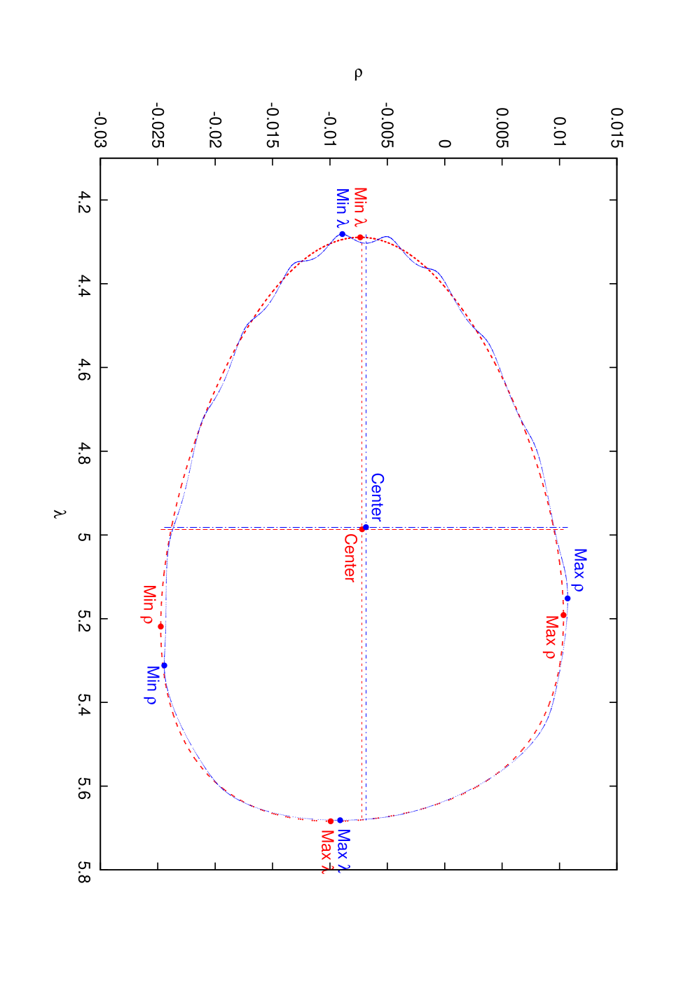
| (19) |
and
| (20) |
The dispersion between centers, which shows how much displacement there is between the orbits, is evaluated by putting
| (21) |
Furthermore, we obtain the value of the enclosed areas for each curve, as follows: we first refer all the points composing the curve, to the already computed center, by introducing the quantities and ; therefore, we obtain the distance to the center and the angle with respect to the horizontal line (). Re-ordering the points by increasing value for the angle , we compute the area contained in the triangle generated by two consecutive points and the center. The sum along all the triangles represents the contained area within each curve, for the complete system and for average Hamiltonian flow. For a further comparison, we compute also the relative difference between the areas , and the displacement of the centers of the orbits with respect to the position of the equilateral Lagrangian point they librate around (, for and for ).
| Asteroid | |||||
|---|---|---|---|---|---|
| 1868 | |||||
| 1872 | |||||
| 2146 | |||||
| 2207 | |||||
| 2674 | |||||
| 2759 |
For 6 of the 7 cases mentioned above, we are able to obtain averaged orbits that reflects the behavior of the numerical integrations. In Table 1, where we report the results for the previously defined quantities, we show that the averaged areas clearly match their associated numerical areas, with a relative error smaller than 2%, except for one case (asteroid 2146 Stentor), for which the error is about 13%. This may be due to the fact that 2146 Stentor presents the largest displacement with respect to the corresponding Lagrangian point, in a quite anomalous orbit. For the rest of the asteroids, the position of the orbits in the surface of section turns to be very close to that generated by the equivalent averaged level curve, both centered at a triangular Lagrangian point. On the other hand, in Table 1 we do not present data for the highly inclined1010 10 According to the Bowell Catalogue at 2452600.5 JD () asteroid 2363 Cebriones of our sample. For this asteroid, our normal form fails to provide an accurate orbit, using the initial conditions provided in [10]. However, we find that the numerical orbit generated by 2363 Cebriones presents a very peculiar angular excursion (in ) with respect to the Lagrangian point. This failure of the normal form could be generated in the initial condition by a non-consistent rotation to the plane of the primaries, in the original work.
4 Summary and perspectives
In this paper we present a novel normalization scheme, that provides an integrable approximation of the dynamics of a Trojan asteroid Hamiltonian in the framework of the Planar Circular Restricted Three-Body Problem (PCRTBP). This new algorithm is based on three co-related points: the introduction of a set of variables which respects the physical configuration of the system; the existence of two degrees of freedom with well distinguishable roles, one corresponding to a fast motion and another corresponding to a slow motion, that allows us to fruitfully average over the fast angle; finally, the analytic singularity of this model exclusively related with the slow angle.
These three concepts motivates a new way to deal with the initial expansion of the Hamiltonian, as it is necessary for the normalization procedure. The slow angle does not affect the solution of the homological equation, determined in order to remove the dependence on the fast angle. Thus, we are able to carefully approximate level curves that represent tadpole and horseshoe orbits by keeping, in the expansions, a non polynomial dependence just with respect to .
In order to examinate the accuracy of the normal form produced, we develop some tests. We study numerically integrated surfaces of section, along the flow of the complete Hamiltonian, and we contrast them with the level curves provided by our integrable normal form, with very good agreement. Furthermore, we estimate some quasi-integrals of motion (by computation of enclosed areas), which also show excellent agreement with those corresponding to the numerically computed surfaces of section. On the whole, this novel approach for producing a new normal form results in a very promising approximation of the global behavior of the Trojans motion.
From a rather theoretical point of view, we think that our normalizing scheme can be complemented with a scheme of estimates, so as to make the remainder exponentially small on a suitable open domain. If our algorithm is joint with a Nekhoroshev-like approach, it should ensure that the eventual diffusion is effectively bounded (i.e., for intervals of time comparable with the age of our Solar system), for a set of initial conditions. We expect such a set to be significantly larger than those considered in the works already existing in the literature. This expectation is due to the fact that our method offers a wide coverage of the Trojans orbits. For the same reason, we think that our integrable approximation can be used in many cases to successfully start the Kolmogorov normalization algorithm. While the corresponding solution is valid for any time, the construction of an invariant KAM torus is an extremely local procedure, because it must be adapted to the orbit of each Trojan body to be studied. In this context, we think that our algorithm can be efficiently used jointly with a KAM-like approach in those cases for which the previous implementation of the Kolmogorov normalization algorithm failed. Let us remark that such a new application of the KAM theory would require to preliminarly construct the action–angle coordinates also for the slow degree of freedom, before starting the final normalization procedure. As an alternative strategy, a different formulation of the KAM theorem that is not strictly based on action–angle variables could be used [5].
More practically, in our opinion the most exciting point is that our method is suitable to be translated to more complex models, without requiring essential changes. Since the PCRTBP corresponds to a very simplistic representation for the Trojans domain, we are presently working to extend the normalization to a Hamiltonian that also considers the eccentricity of the primary. The first preliminary results show that our method can be used so as to locate the main secondary resonances within the 1:1 MMR region. In particular, we find a good agreement with other purely numerical indicators, when the mass ratio between the primaries is small. We plan to include these and other results in a future publication. Furthermore, we think that our present and future contributions will help to fill that still existing gap between the semi-analytic studies and the more complete numerical experiments of the stability region.
Acknowledgements
The authors would like to thank C. Efthymiopoulos for his advice and constant support. We are indebted also with C. Simó who suggested to reconsider the article [11], and with the anonymous referee, whose contribution helped improving the original manuscript. During this work, R.I.P. was supported by the Astronet-II Marie Curie Training Network (PITN-GA-2011-289240), while U.L. was partially supported also by the research program “Teorie geometriche e analitiche dei sistemi Hamiltoniani in dimensioni finite e infinite”, PRIN 2010JJ4KPA_009, financed by MIUR.
References
- [1] Abad, A., Barrio, R., Blesa, F., Rodriguez, M., “Algorithm 924: TIDES, a Taylor Series Integrator for Differential EquationS”, ACM Transactions on Math. Software, 39, Issue 1, Article No.: 5 (2012)
- [2] Arnold, V.I., “Mathematical Methods of Classical Mechanics”, 2-nd edition, Springer-Verlag, New York (1989).
- [3] Ceccaroni, M., Biggs, J., “Analytic perturbative theories in highly inhomogenehous gravitational fields”, Icarus, 224, 74–85 (2013).
- [4] Celletti, A., Giorgilli, A., “On the stability of the lagrangian points in the spatial restricted problem of three bodies”, Cel. Mech. & Dyn. Astr., 50, 31–58 (1991).
- [5] de la Llave, R., González, A., Jorba, À., Villanueva, J., “KAM theory without action-angle variables”, Nonlinearity, 18, 855–895 (2005).
- [6] Dvorak, R., Lhotka, C., Zhou, L., “The orbit of 2010 TK7: possible regions of stability for other Earth Trojan asteroids”, Astron. Astrophys., 541, A127 (2012).
- [7] Efthymiopoulos, C., “High order normal form stability estimates for co-orbital motion”, Cel. Mech. & Dyn. Astr., 117, 101–112 (2013).
- [8] Efthymiopoulos, C., Sándor, Z., “Optimized Nekhoroshev stability estimates for the Trojan asteroids with a symplectic mapping model of co-orbital motion”, Mon. Not. R. Astron. Soc., 364, 253–271 (2005).
- [9] Érdi, B., “The Trojan Problem”, Cel. Mech. & Dyn. Astr., 65, 149–1642 (1997).
- [10] Gabern, F., Jorba, A., Locatelli, U., “On the construction of the Kolmogorov normal form for the Trojan asteroids”, Nonlinearity, 18, 1705–1734 (2005).
- [11] Garfinkel, B., “Theory of the Trojan asteroids, 1.”, Astronomical Journal, 82, 368–379 (1977).
- [12] Giorgilli, A., “Notes on exponential stability of Hamiltonian systems”, in Dynamical Systems, Part I: Hamiltonian systems and Celestial Mechanics, Pubblicazioni del Centro di Ricerca Matematica Ennio De Giorgi, 87–198 (2003).
- [13] Giorgilli, A., Skokos, Ch., “On the stability of the Trojan asteroids”, Astron. Astrophys., 317, 254–261 (1997).
- [14] Jorba, A., Zou, M., “A Software Package for the Numerical Integration of ODEs by Means of High-Order Taylor Methods”, Experiment. Math., 14, 99–117 (2005).
- [15] Libert, A.-S., Sansottera, M., “On the extension of the Laplace-Lagrange secular theory to order two in the masses for extrasolar systems”,Cel. Mech. & Dyn. Astr., 117, 149–168 (2013).
- [16] Lhotka, Ch., Efthymiopoulos, C., Dvorak, R., “Nekhoroshev stability at or in the elliptic-restricted three-body problem - application to Trojan asteroids”, Mon. Not. R. Astron. Soc., 384, 1165–1177 (2008).
- [17] Murray, C.D., and Dermott, S.F., “Solar System Dynamics”, Cambridge University Press, Cambridge (1999).
- [18] Nekhoroshev, N.N., “Exponential estimates of the stability time of near–integrable Hamiltonian systems”, Russ. Math. Surveys, 32, 1–65 (1977).
- [19] Nekhoroshev, N.N., “Exponential estimates of the stability time of near–integrable Hamiltonian systems, 2.”, Trudy Sem. Petrovs., 5, 5–50 (1979).
- [20] Páez, R.I., Efthymiopoulos, C., “Trojan resonant dynamics, stability, and chaotic diffusion, for parameters relevant to explanetary systems”, Cel. Mech. & Dyn. Astro., 121, 139–170 (2015).
- [21] Páez, R.I., Locatelli, U., “Design of maneuvers based on new normal form approximations: The case study of the CPRTBP”, AIP Conference Proceedings, 1637, Issue 1, 776–785 (2014).
- [22] Robutel, P., Gabern, F., Jorba, A., “The observed trojans and the global dynamics around the lagrangian points of the Sun-Jupiter system”, Cel. Mech. & Dyn. Astr., 92, 153–69 (2005).
- [23] Robutel, P., Gabern, F., “The resonant structure of Jupiter’s Trojan asteroids - I. Long-term stability and diffusion”, Mon. Not. R. Astron. Soc, 372, 1463–1482 (2006).
- [24] Sansottera, M., Locatelli, U., Giorgilli, A., “A semi-analytic algorithm for constructing lower dimensional elliptic tori in planetary systems”, Cel. Mech. & Dyn. Astr., 111, 337–361 (2011).
Appendix A Details about the formal algorithm constructing the normal form
As discussed in subsection 2.2, the normalization algorithm defines a sequence of Hamiltonians. This is done by an iterative procedure; let us describe the basic step which introduces starting from when both the values of the indexes and are positive. We assume that the expansions of is such that
|
|
(22) |
where , , , , and . Let us recall that the Hamiltonian written in (6) is suitable for starting the procedure with . In formula (22), one can distinguish the normal form terms from the perturbing part; the latter depends on in a generic way, while in the terms of type appearing in (22) the fast variables can be replaced by the action . The –th step of the algorithm formally defines the new Hamiltonian by applying the Lie series operator to the previous Hamiltonian , as it is prescribed in formula (10). The new generating function is determined by solving the following homological equation with respect to the unknown :
| (23) |
where we require that is the new term in normal form, i.e. .
Proposition A.1
If and , then there exists a generating function and a normal form term satisfying the homological equation (23).
We limit ourselves to just sketch the procedure that can be followed so as to explicitly determine a solution of (23) and, therefore, prove the statement above. First, we replace the fast coordinates with the pair of complex conjugate canonical variables such that and . Moreover, the homological equation (23) has to be expanded in Taylor series with respect to , using the slow coordinates as fixed parameters (because they are not affected by the Poisson bracket , since do not depend on them). Therefore, we solve term-by-term the equation (23) in the unknown coefficients1111 11 We emphasize that the most celebrated problem concerning the convergence of the normal forms, i.e., the occurrence of “small divisors”, does not affect our scheme, because the main integrable term in the homological equation (23), i.e. , depends just on the fast action . and such that
|
|
and
|
|
At last, we express the expansions above by replacing with , and we obtain the final solutions in the form and .
The following property of the Poisson brackets is very useful for our purposes; however, since its proof just requires long but basically trivial calculations, it is omitted.
Proposition A.2
Let and be two generic functions such that and , then
In order to provide an algorithm easy to translate in a programming language, we are going to give explicit formulas for the new terms of type appearing in expansion (9) of Hamiltonian . Let us introduce the recursive operation , where the previously defined quantity is redefined as . Therefore, we initially define
Then, we consider the contribution of the terms generated by the Lie series applied to each function belonging to the normal form part as follows:
| (24) |
where the upper limits and on the indexes and , respectively, are such that
|
|
(25) |
For what concerns the contributions given by the perturbing terms making part of the expansion of in (22), we have
| (26) |
where the limiting values for the indexes, that are and , are defined in (25).
The redefinition rules (24) and (26) are set so that the new perturbing part generated by the Lie series in (10) is coherently split in different terms according to their order of magnitude in and their total polynomial degree in the actions. In fact, by applying repeatedly proposition A.2 to the redefinitions in ()–(26), it is possible to inductively verify that . Therefore, the terms making part of the Hamiltonian in the expansion (9) share the same properties with those appearing in (22); this ensures that the normalization algorithm can be iterated so as to construct . The simple prescription , , allows to deal with generating functions of the next order of magnitude, i.e., . As discussed in subsection 2.2, by applying repeatedly the rules of the generic normalization step, the algorithm finally ends, by determining the last Hamiltonian .