Limiting the spread of disease through altered migration patterns

Recently, a number of papers have been devoted to the issue of controlling disease outbreaks. Typical mechanisms for control involve treatments which speed recovery [25, 28], culling of infected individuals [24], reducing the density of disease vectors [23], vaccination programs [19, 20] and quarantine [28]. When the population has some spatial structure, migration also plays an important role in disease spread and provides a further control mechanism.

A common approach to incorporating spatial structure in epidemic modelling is to impose a metapopulation structure on the population [see 9, 13, 14, 17, for example]. In a metapopulation, the population is divided into a number of subpopulations occupying geographically distinct locations. The disease is spread within a subpopulation by contacts between infective and susceptible individuals and is spread between subpopulations by the migration of infected individuals.

The effect of migration rates on disease spread in metapopulations has been investigated in a number of papers. Due to the complexity of these models, control strategies are often based on minimising the basic reproduction number $R_{0}$. Studying a multi-patch frequency dependent SIS model, Allen et al [2] note that the rapid movement of infective individuals can lead to disease extinction in low risk environments. Furthermore, they conjecture that $R_{0}$ is a decreasing function of the diffusion rate for infective individuals. Hsieh et al [18, Theorem 4.2] note a similar result for their two-patch SEIRP model and a similar phenomena has been observed in population models with spatially heterogeneous environments [16]. However, Gao and Ruan [12, section 4] have shown that for other models the dependence of $R_{0}$ on migration rates can be more complex. To investigate the effect of the migration rates on other quantities such as the number of infected individuals, numerical methods are generally required [29, for example].

In this paper, we examine how susceptible individuals can act collectively to limit the spread of disease during the initial phase of an epidemic. More specifically, we consider how susceptible individuals can distribute themselves in the metapopulation in a way that minimises the growth of the epidemic when the infectives migrate so as to maximise the growth. By formulating the problem as a minimax optimisation and focusing on the susceptible individuals, we avoid the need to distinguish between infected and susceptible individuals when applying controls to the population. This is advantageous as identification of infected individuals can be problematic due to factors such as delays in the onset of symptoms, asymptomatic carriers and costs associated with testing. Furthermore, acute disease can have a significant effect on the behaviour of animals [15]. This is particularly true for certain parasitic diseases where the parasite attempts to force the host to act in a manner which assists the propagation of the parasite [1].

In Section 2 we give our main results. Instead of using an ODE model for the epidemic as was done in the papers cited above, our analysis is based on a branching process model. Branching processes are known to provide a good approximation to the standard SIR and SIS Markov chain models when the number of infectives is initially small [7]. Using this model, we are able to give an explicit strategy that minimises the expected rate of growth under a certain condition on the recovery and infection rates. We also give an explicit strategy that minimises the basic reproduction number which does not require this extra condition. This later strategy is shown to also be optimal in terms of the probability of extinction and total size of the epidemic. In Section 3, the problem of minimising the expected growth rate is investigated numerically. The paper concludes with a discussion of how the results depend on contact rates and how they relate to ODE models.

Consider a closed population of size $N$ divided into $m$ groups such that at time $t$ group $i$ contains $X_{i}(t)$ susceptibles and $Y_{i}(t)$ infectives. Each individual, conditional on its disease status, moves independently between groups according to an irreducible Markov process on $\{1,\ldots,m\}$ with transition rate matrix $R$ if it is susceptible and transition rate matrix $Q$ if it is infected. The epidemic evolves as a Markov process. Contacts between individuals in the same group are assumed to be density dependent [6]. More precisely, a pair of individuals in group $i$ makes contact at the points of a Poisson process of rate $\beta_{i}/N$ with contacts between distinct pairs of individuals being mutually independent. It is assumed that contact between an infective and a susceptible results in the infection of the susceptible. An infected individual in group $i$ recovers with immunity at a rate $\gamma_{i}$. Since we are primarily concerned with the initial phase of the epidemic, our conclusions remain valid for epidemics where individuals recover without immunity.

In the absence of infective individuals, the entirely susceptible population evolves following a closed (linear) migration process with per-capita migration rates $R$. If the population is in equilibrium, then the probability that an individual is in group $i$ is given by $\pi_{i}$ where $\pi$ is the unique solution to $\pi R=0$ subject to the constraint $\pi{\bf 1}=1$.

We consider the spread of the disease from a small number of initial infective individuals. Clancy [7, Theorem 2.1] shows that, when $N$ is large, the epidemic can be approximated by a multi-type branching process. Assuming the susceptible population is in equilibrium, the branching process for the number of infective individuals is given by

Note that the branching process depends on $R$ only through the equilibrium distribution $\pi$.

Suppose that the susceptible population aims to minimise some quantity $f(\pi,Q)$, calculated from the branching process determined by (2.1)-(2.3). Let $\mathcal{S}$ denote the relative interior of the $(m-1)$-simplex and let $\mathcal{Q}$ be the set of irreducible migration rate matrices. Without imposing any constraints on the movements of the infectives, the susceptible population can choose $\pi$ such that, for any $\epsilon>0$, a value no larger than $\inf_{\pi\in\mathcal{S}}\sup_{Q\in\mathcal{Q}}f(\pi,Q)+\epsilon$ is attained. On the other hand, the infectives can migrate in such a way that, for any $\epsilon>0$, a value no smaller than $\sup_{Q\in\mathcal{Q}}\inf_{\pi\in\mathcal{S}}f(\pi,Q)-\epsilon$ is attained. In general,

[32, Lemma in section 1.2.2]. A pair $(\pi^{\ast},Q^{\ast})\in\mathcal{S}\times\mathcal{Q}$ such that

for all $\pi\in\mathcal{S}$ and all $Q\in\mathcal{Q}$ is called a saddle point for $f$. If a saddle point exists, then

[32, Theorem in section 1.3.4]. The susceptibles can attain this value by distributing themselves amongst the groups according to $\pi^{\ast}$. When a saddle point for $f$ does not exist, there may still be an $\epsilon$-saddle point, that is, for every $\epsilon>0$ there exists a pair $(\pi^{\epsilon},Q^{\epsilon})\in\mathcal{S}\times\mathcal{Q}$ such that

for all $\pi\in\mathcal{S}$ and all $Q\in\mathcal{Q}$. The existence of an $\epsilon$-saddle point implies that

[32, Theorem in section 2.2.5]. In the following, we determine the $(\epsilon)$-saddle points for four quantities derived from the branching process (2.1)-(2.3).

As mentioned in the introduction, this formulation avoids the need to distinguish between susceptible and infected individuals in the application of controls. To illustrate this point, suppose that susceptible individuals normally move between groups following a Markov process with migration rate matrix $R$. The optimal distribution of susceptibles $\pi^{\ast}$ can be obtained by border controls where a migrating individual from group $j$ going to group $i$ is given admittance with probability $p_{ji}$ and otherwise returned to group $j$. Detailed balance equations show that the optimal distribution for susceptibles is obtained if the admittance probabilities satisfy

for all $i,j$. Although the border controls will have an effect on the migration rate of infected individuals if they are applied to the population as a whole, the optimal distribution for susceptible individuals ensures that the growth of the epidemic can be no greater than $\min_{\pi\in\mathcal{S}}\sup_{Q\in\mathcal{Q}}f(\pi,Q)$.

In this section we investigate numerically two issues. The first issue concerns the optimal distribution of susceptibles with respect to minimising the expected growth rate. Theorem 2.1 gives the optimal distribution only if $\gamma_{i}>-\chi(\beta,\gamma)$ for all $i$. We have also seen that if $\gamma_{i}\geq-\chi(\beta,\gamma)$ for all $i$ and $\gamma_{j}=-\chi(\beta,\gamma)$ for some $j$, then there is a sequence of distributions $\pi^{\epsilon}$ which achieve within $\epsilon$ the optimal value of $\tau$ and for which $\lim_{\epsilon\rightarrow 0}\pi^{\epsilon}_{j}=0$. We might expect that if the recovery rate for this group were to decrease, then the optimal distribution would place no susceptibles in group $j$. This was investigated in a two group epidemic with $\beta_{1}=1$, $\beta_{2}=2$, and $\gamma_{1}$ and $\gamma_{2}$ in $(0,4)$. For these epidemics both $\sup_{Q\in\mathcal{Q}}\inf_{\pi\in\mathcal{S}}\tau(\pi,Q)$ and $\inf_{\pi\in\mathcal{S}}\sup_{Q\in\mathcal{Q}}\tau(\pi,Q)$ were computed by nested optimisation using the optim and optimize functions in R [27]. The two quantities differed by less than $10^{-4}$ in all instances computed. The optimal value of $\tau(\pi,Q)$ is plotted in Figure 1. Note that in most of the region plotted growth rate is negative. This is to be expected as when the condition of Theorem 2.1 does not hold, the optimal growth rate must be negative from Corollary 2.2. The numerical results confirms our intuition that $\pi^{\ast}_{i}=0$ if $\gamma_{i}\leq-\chi(\beta,\gamma)$ for the two group model. From the plot it is seen that if $\gamma_{1}<-\chi(\beta,\gamma)\leq\gamma_{2}$, then increasing $\gamma_{2}$ has no effect on the optimal value of $\tau(\pi,Q)$. This is explained as when $\gamma_{1}<-\chi(\beta,\gamma)\leq\gamma_{2}$, the optimal distribution of susceptibles has $\pi^{\ast}_{2}=1$. On the other hand, the inequality $\gamma_{1}<-\chi(\beta,\gamma)$ implies $\gamma_{1}<\gamma_{2}-\beta_{2}$, so the infectives slow the decrease of the epidemic by moving to group one. Therefore, increasing the recovery rate in group two has no effect on the growth rate of the epidemic and $\inf_{\pi\in\mathcal{S}}\sup_{Q\in\mathcal{Q}}\tau(\pi,Q)=-\gamma_{1}$.

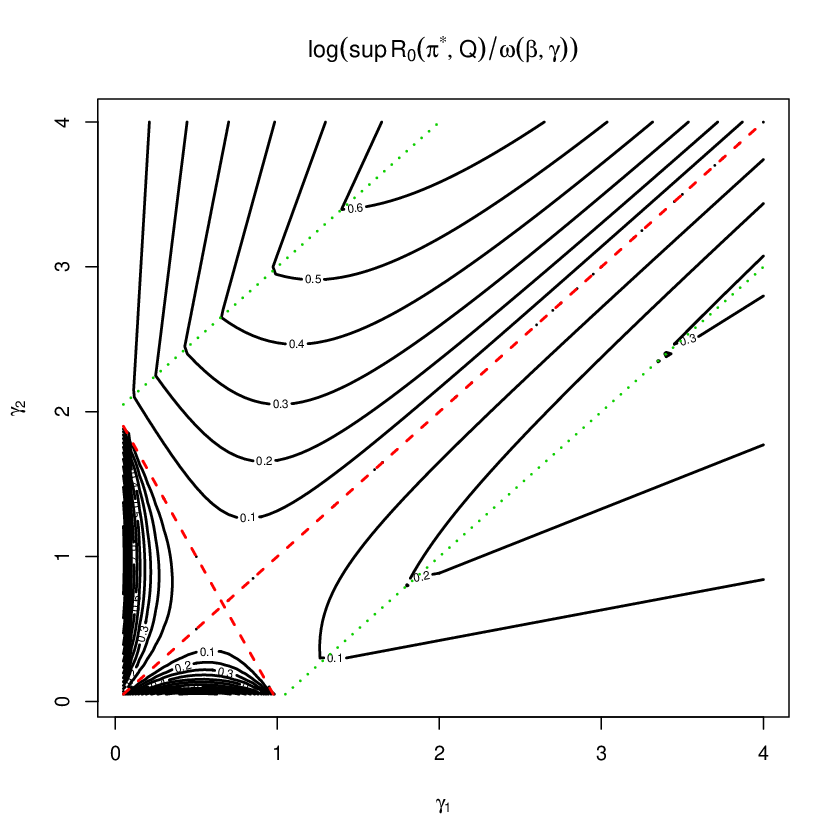
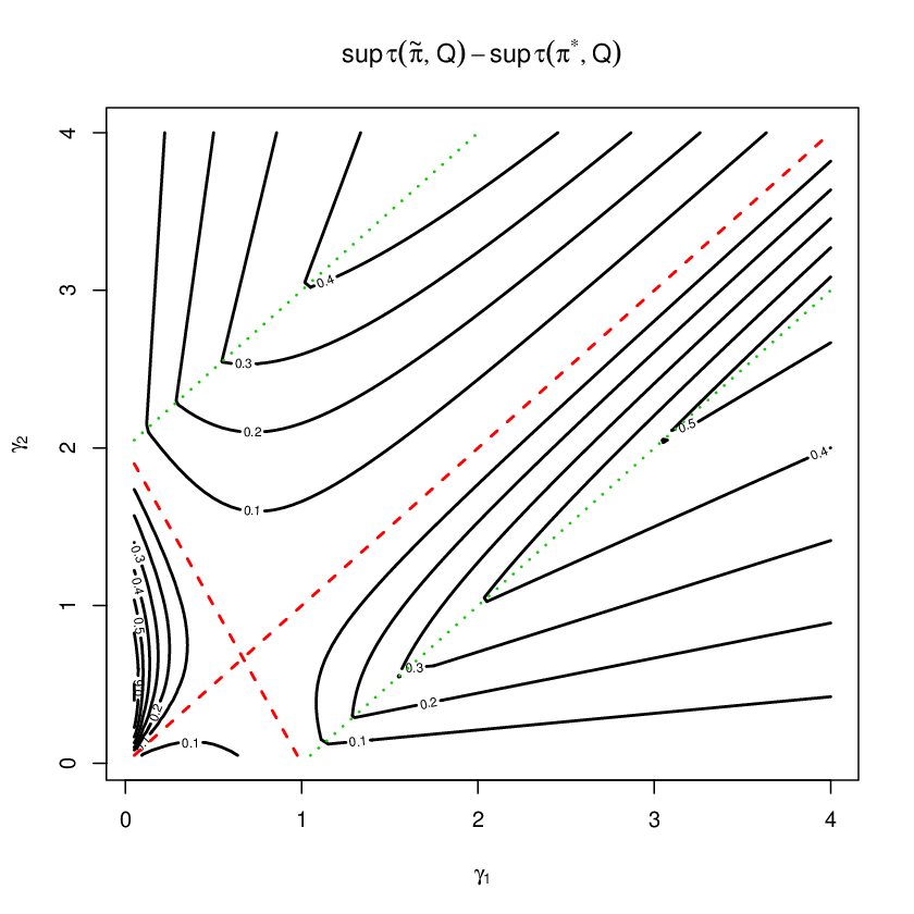
By construction, $\pi^{\ast}$ and $\tilde{\pi}$ are the optimal distribution of susceptibles for minimising $\tau$ and $R_{0}$ respectively. We now consider their performance on the alternate criteria, that is we calculate $\sup_{Q\in\mathcal{Q}}R_{0}(\pi^{\ast},Q)$ and $\sup_{Q\in\mathcal{Q}}\tau(\tilde{\pi},Q)$. Figures 2 and 3 show how much these quantities are increased by taking alternate optimal distributions of susceptibles. Qualitatively, both figures are very similar. Both quantities plotted achieve their minimum for the same set of $\gamma$, indicated by the dashed line, as $\pi^{\ast}=\tilde{\pi}$ for these values of $\gamma$. Also, an abrupt change in the contours occur along the dashed line in both figures. This is due to $\pi^{\ast}$ placing zero probability in one of the groups for those values of $\gamma$ outside the dashed lines.

For most values of $\gamma$ the optimal choice for one criterion appears to result in reasonable performance in the other. In particular, in the region where $\gamma_{1}\approx\gamma_{2}\approx\beta_{1}\beta_{2}/(\beta_{1}+\beta_{2})$, $\tau$ and $R_{0}$ take approximately the same value under $\pi^{\ast}$ and $\tilde{\pi}$. However, for small values of $\gamma$, the performance of the alternate distributions rapidly deteriorates for both $\tau$ and $R_{0}$. This is expected as when $\gamma$ is small, $\chi(\beta,\gamma)$ tends to be large which causes the difference between $\pi^{\ast}$ and $\tilde{\pi}$ to also be large.

The conclusions of Theorems 2.1 and 2.3 are in part not surprising; in order to minimise the spread of the disease most susceptible individuals should belong to groups with relatively low infection rates and high recovery rates. However, for the form of contact rate assumed here, this needs to be balanced with the fact that contact rates are higher in groups with larger populations. Although Theorems 2.4 and 2.5 showed that this balance is achieved in the same way for $R_{0}$-optimal, extinction probability optimal, and expected total size optimal distributions of susceptibles, it was achieved differently for $\tau$-optimal distribution of susceptibles. It is conceivable that this balance might be achieved differently for other measures of disease spread.

In our analysis, we have focussed on the branching process approximation to the epidemic. Another widely used approximation is provided by the solution to an ordinary differential equation (ODE). Assume that infected individuals recover without immunity. For the epidemic described at the beginning of Section 2, the ODE approximation is given by the solution to

It is known that if $N^{-1}X_{i}(0)\stackrel{{\scriptstyle p}}{{\rightarrow}}x_{i}(0)$ and $N^{-1}Y_{i}(0)\stackrel{{\scriptstyle p}}{{\rightarrow}}y_{i}(0)$ for $i=1,\ldots,m$ as $N\rightarrow\infty$, then for any finite $T>0$ and any $\epsilon>0$

References

- [1] Adamo SA (2013) Parasites: evolution’s neurobiologists, Journal of Experimental Biology, 216, 3-10. doi:10.1242/jeb.073601
- [2] Allen LJS, Bolker BM, Lou Y and Nevai AL (2007) Asymptotic Profiles of the Steady States for an SIS Epidemic Patch Model, SIAM Journal on Applied Mathematics, 67, 1283-1309. doi:10.1137/060672522
- [3] Allen LJS and Lahodny Jr GE (2013) Extinction thresholds in deterministic and stochastic epidemic models, Journal of Biological Dynamics, 6, 590-611. doi:10.1080/17513758.2012.665502
- [4] Allen LJS and van den Driessche P (2013) Relations between deterministic and stochastic thresholds for disease extinction in continuous- and discrete-time infectious disease models, Mathematical Biosciences, 243, 99-108. doi:10.1016/j.mbs.2013.02.006
- [5] Athreya KB (1968) Some Results on Multitype Continuous Time Markov Branching Processes, Annals of Mathematical Statistics, 39, 347-357. doi:10.1214/aoms/1177698395
- [6] Begon M, Bennett M, Bowers RG, French NP, Hazel SM and Turner J (2002) A clarification of transmission terms in host-microparasite models: numbers, densities and areas, Epidemiology and Infection, 129 147-153. doi:10.1017/S0950268802007148
- [7] Clancy D (1996) Strong approximations for mobile populations epidemic models, Annals of Applied Probability, 6, 883-895.
- [8] Darling RWR and Norris JR (2008) Differential equation approximations for Markov chains, Probability Surveys, 5, 37-79. doi:10.1214/07-PS121
- [9] Débarre F, Bonhoeffer S, Regoes RR (2007) The effect of population structure on the emergence of drug resistance during influenza pandemics, Journal of the Royal Society Interface, 4, 893-906. doi:10.1098/rsif.2007.1126
- [10] Diekmann O, Heesterbek JAP and Roberts MG (2010) The construction of next-generation matrices for compartmental epidemic models, Journal of the Royal Society Interface, 7, 873-885. doi:10.1098/rsif.2009.0386
- [11] Friedland S (1981) Convex spectral functions, Linear and Multilinear Algebra, 9, 299-316. doi:10.1080/03081088108817381
- [12] Gao D and Ruan S (2012) A multipatch malaria model with logistic growth populations, SIAM Journal of Applied Mathematics, 72, 819-841. doi:10.1137/110850761
- [13] Grenfel Bl and Harwood J (1997) (Meta)population dynamics of infectious diseases, Trends in Ecology and Evolution, 12, 395-399. doi:10.1016/S0169-5347(97)01174-9
- [14] Gurarie D and Seto EYW (2009) Connectivity sustains disease transmission in environments with low potential for endemicity: modelling schistosomiasis with hydrologic and social connectivities, Journal of the Royal Society Interface, 6, 495-508. doi:10.1098/rsif.2008.0265
- [15] Hart B (1988) Biological basis of the behavior of sick animals, Neuroscience & Biobehavioral Reviews, 12, 123-137. doi:10.1016/S0149-7634(88)80004-6
- [16] Hastings A (1983) Can spatial variation alone lead to selection for dispersal? Theoretical Population Biology, 24, 244-251. doi:10.1016/0040-5809(83)90027-8
- [17] Hess G (1996) Disease in metapopulation models: implications for conservation, Ecology, 77, 1617-1632. doi:10.2307/2265556
- [18] Hsieh Y-H, van den Driessch P and L Wang (2007) Impact of travel between patches for spatial spread of disease, Bulletin of Mathematical Biology, 69, 1355-1375. doi:10.1007/s11538-006-9169-6
- [19] Klepac P, Bjørnstad ON, Metcalf CJE and Grenfell BT (2012) Optimizing reactive responses to outbreaks of immunizing infections: balancing case management and vaccination, PLOS One, 7, e41428. doi:10.1371/journal.pone.0041428
- [20] Klepac P, Laxminarayan R and Grenfell BT (2011) Synthesizing epidemiological and economic optima for control of immunizing infections, Proceedings of the National Academy of Sciences, 108, 14366-14370. doi:10.1073/pnas.1101694108
- [21] Kurtz TG (1970) Solutions of ordinary differential equations as limits of pure jump Markov processes, Journal of Applied Probability, 7, 49-58.
- [22] Lahodny Jr GE and Allen LJS (2013) Probability of a Disease Outbreak in Stochastic Multipatch Epidemic Models, Bulletin of Mathematical Biology, 75, 1157-1180. doi:10.1007/s11538-013-9848-z
- [23] Mpolya EA, Yashima K, Ohtsuki H and Sasaki A (2014) Epidemic dynamics of a vector-borne disease on a villages-and-city star network with commuters, Journal of Theoretical Biology, 343, 120-126. doi:10.1016/j.jtbi.2013.11.024
- [24] Ndeffo Mbah ML and Gilligan CA (2010) Optimization of control strategies for epidemics in heterogeneous populations with symmetric and asymmetric transmission, Journal of Theoretical Biology, 262, 757-763. doi:10.1016/j.jtbi.2009.11.001
- [25] Ndeffo Mbah ML and Gilligan CA (2011) Resource allocation for epidemic control in metapopulations, PLOS One, 6, e24577. doi:10.1371/journal.pone.0024577
- [26] Pollett PK and Stefanov VT (2002) Path integral for continuous-time Markov chains, Journal of Applied Probability, 39, 901-904.
- [27] R Development Core Team (2011) R: A language and environment for statistical computing. R Foundation for Statistical Computing, Vienna, Austria.
- [28] Rowthorn RE, Laxminarayan R and Gilligan CA (2009) Optimal control of epidemics in metapopulations, Journal of the Royal Society Interface, 6, 1135-1144. doi:10.1098/rsif.2008.0402
- [29] Sanders J, Noble B, van Gorder RA and Riggs C (2012) Mobility matrix evolution for an SIS epidemic patch model, Physica A, 391, 6256-6267. doi:10.1016/j.physa.2012.07.023
- [30] Seneta E, (1981) Non-negative matrices and Markov chains, 2nd Edition, Springer, New York
- [31] Stewart GW and Sun J-G (1990) Matrix Perturbation Theory, Academic Press, Boston
- [32] Petrosjan LA and Zenkevich NA (1996) Game theory, World Scientific, Singapore
- [33] van den Driessche P and Watmough J (2002) Reproduction numbers and sub-threshold endemic equilibria for compartmental models of disease transmission, Mathematical Biosciences, 180, 29-48. doi:10.1016/S0025-5564(02)00108-6