Model Selection versus Model Averaging in Dose Finding Studies
Abstract
Phase II dose finding studies in clinical drug development are typically conducted to adequately characterize the dose response relationship of a new drug. An important decision is then on the choice of a suitable dose response function to support dose selection for the subsequent Phase III studies. In this paper we compare different approaches for model selection and model averaging using mathematical properties as well as simulations. Accordingly, we review and illustrate asymptotic properties of model selection criteria and investigate their behavior when changing the sample size but keeping the effect size constant. In a large scale simulation study we investigate how the various approaches perform in realistically chosen settings. Finally, the different methods are illustrated with a recently conducted Phase II dose-finding study in patients with chronic obstructive pulmonary disease.
Keywords and Phrases: Model selection; model averaging; clinical trials; simulation study
1 Introduction
A critical decision in pharmaceutical drug development is the selection of an appropriate dose for confirmatory Phase III clinical trials and potential marketing authorization. For this purpose, dose finding studies are conducted in Phase II to investigate the dose response relationship of usually active doses in the intended patient population for a clinically relevant endpoint; see Ting, (2006) among many others.
Traditionally, dose response studies were analyzed by treating dose as a categorical variable in an analysis-of-variance (ANOVA) model. Only in the past 20 years the use of regression modeling approaches where dose is treated as a quantitative variable has become more popular. We refer to, for example, Bretz et al., (2008) for an overview of both approaches, and the White Paper of the Pharmaceutical Research and Manufacturers of America (PhRMA) working group on adaptive dose ranging studies (Bornkamp et al., (2007)) for a comparison of different ANOVA and regression-based approaches.
If a non-linear regression model is adopted, a natural question is which regression (i.e. dose response) function to utilize. This becomes even more important in the regulated context of pharmaceutical drug development, where the employed regression model should be pre-specified at the design stage. This specification thus takes place at a time, when only limited information is available about the dose response relationship, resulting in model uncertainty. Several authors (e.g. Thomas, (2006); Dragalin et al., (2007)) argued that a flexible monotonic model, such as an Sigmoid Emax model, can be used for all practical purposes, as it approximates the commonly observed dose response shapes well. While generally applicable, this flexible model can sometimes be challenging to fit with a small number of doses. In addition, while several models might fit the data similarly well, due to the often sparse data they might still differ on certain estimated quantities of interest, e.g. the target dose estimate.
The MCP-Mod method (see Bretz et al., (2005); Pinheiro et al., (2014); CHMP, (2014)) tries to address the model uncertainty problem by acknowledging it explicitly as part of the methodology. The main idea is to determine a candidate set of dose response models at the trial design stage. After completing the trial one either selects a single dose response function out of the candidate model set or applies model averaging based on the individual model fits. Thus, the MCP-Mod approach allows one to employ either model selection or model averaging. Verrier et al., (2014) discussed by means of two real examples their experiences on how to proceed with model selection and model averaging using MCP-Mod in practice.
Model selection has the advantage that it results in a single model fit, which eases the interpretation and communication. But it is also known that selecting a single model and ignoring the uncertainty resulting from the selection will result in confidence intervals with coverage probability smaller than the nominal value, see for example Bornkamp, (2015) for a high-level discussion or Chapter 7 in Claeskens and Hjort, (2008) for a mathematical treatment. A partial solution to this problem is to use model averaging. By acknowledging model uncertainty explicitly as part of the inference one will typically obtain more adequate (i.e usually wider) confidence intervals. There exists empirical evidence that model averaging also improves the estimation efficiency (see Raftery and Zheng, (2003) or Breiman, (1996)), even though authors did not consider dose-finding setting in particular.
The purpose of this paper is to investigate and compare different model selection and model averaging approaches in the context of Phase II dose finding studies. Accordingly, we introduce in Section 2 a motivating case study to illustrate the various approaches investigated throughout this paper. Next, we briefly review the mathematical background of different selection criteria and compare them with respect to some of their asymptotic properties in Section 3. In Section 4, we describe the results of an extensive simulation study. We revisit the case study in Section 5 and provide some general conclusions in Section 6.
2 A Case Study in Chronic Obstructive Pulmonary Disease (COPD)
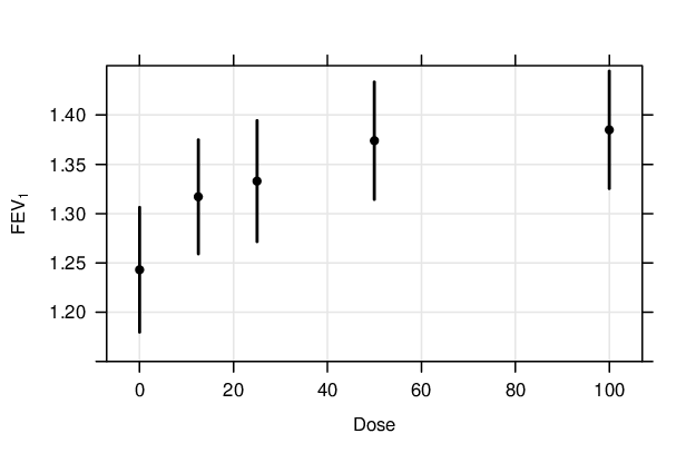
This example refers to a Phase II clinical study of a new drug in patients with chronic obstructive pulmonary disease (COPD). The primary endpoint of the study was measured through the forced expiratory volume in one second () measured in liter, after 7 days of treatment. The objective of this study was to determine the dose response relationship and the target dose that achieves an effect of over placebo. In COPD an improvement of liters on top of the placebo response are considered clinically relevant. To this end, four active dose levels (12.5, 25, 50 and 100 mg) were compared with placebo. Point estimates and standard errors for the treatment groups resulting from an ANCOVA fit are available from clinicaltrials.gov (NCT00501852). The original study design was a four-period incomplete block cross-over study; see also Verkindre et al., (2010). For the purpose of this article we simulated a parallel group design of 60 patients per group (thus 300 patients in total), so that the point estimates and standard errors match the reported estimates exactly. Figure 2.1 displays the mean responses at the five dose levels (including placebo) together with the marginal 95% confidence intervals.
For our purposes, we assume that five candidate models had been identified at the design stage to best describe the data after completing the trial. More specifically, we assume the five dose-response functions summarized in Table 2.1, namely the linear, quadratic, Emax, Sigmoid Emax and ANOVA model; see Section 3 for the notation used in Table 2.1. The questions at hand are (i) which of these candidate models should be used for the dose response modeling step, (ii) whether model selection or averaging should be used, and (iii) which specific information criteria should be employed to perform either model selection or averaging. We will revisit and analyse this case study in Section 5.
| Number | Model | Function | Parameter specifications |
|---|---|---|---|
| 1 | Linear | ||
| 2 | Quadratic | ||
| 3 | Emax | ||
| 4 | Sigmoid Emax | ||
| 5 | ANOVA | ||
3 Model Selection and Model Averaging
We assume different dose levels , where often is the placebo. The set of dose levels is called design throughout this paper. We further assume that for each dose level we have patients , where . The individual responses are denoted by
| (3.1) |
Throughout this paper, we assume that the observations in (3.1) are realizations of random variables defined by
| (3.2) |
where are independent and normally distributed random variables, i.e. . Here, denotes the mean response at dose . The competing dose response mean functions in (3.2) are denoted by , . For example, in the case study presented in Section 2 we assumed the candidate models , summarized in Table 2.1.
In the remainder of this section we give a brief overview of commonly used information criteria for selecting a model from a given class of competing models. All criteria can be represented in the form
| (3.3) |
where denotes the likelihood function and a penalty term which differs for the different models and selection criteria . Table 3.1 summarizes the penalty terms of different criteria that will be introduced below and investigated in later sections.
| Model Selection Criterion | Penalty Term for model |
|---|---|
| AIC | |
| BIC | |
| TIC |
3.1 Information criteria based on the AIC
AIC-based information criteria are often motivated from an information theoretic perspective. Let denote the true but unknown density of the response variable given the dose . In order to estimate target doses of interest and the dose response curve, we want to identify a model defined by a parametric density for the response variable from a given class of parametric models which approximates the true density best. In order to measure the quality of the approximation we use the Kullback Leibler divergence (KL-divergence)
| (3.4) |
The KL-divergence serves as a distance measure between densities. It is nonnegative and equal to zero if . Based on the KL-divergence a model from a given class of models, say , is called the best approximating model if its density (with corresponding optimizing parameter minimizes the KL-divergence to the true density compared to the KL-divergence of the other models.
In practice, the identification of the best approximating model within a set of candidate models by minimizing the KL-divergence (3.4) is not possible because this criterion depends on the unknown true density. However the divergence and the parameters corresponding to the best approximation can be estimated from the data . Ignoring the terms that are the same across all models, one hence needs to minimize
where the
expectation is taken with respect to the distribution of the maximum likelihood
(ML) estimator of
the parameter in model .
It is known that the empirical estimator of this quantity, the log
likelihood is a biased estimator and
overestimates , leading to overfitting (cf.
Claeskens and Hjort, (2008)).
A bias corrected estimator instead
is given by
| (3.5) |
Using different estimators for the penalty term thus leads to different model selection criteria; see Table 3.1. Claeskens and Hjort, (2008) discussed under which circumstances the different penalties lead to an approximately unbiased estimation of , in Appendix A we provide further technical background on asymptotic approximations of the bias term. Setting leads to the popular Akaike information criterion (AIC; Akaike, (1974))
The coefficient is added because of approximation arguments (see among others Claeskens and Hjort, (2008)). Hurvich and Tsai, (1989) pointed out that the dimension is not a good estimator of the bias for small sample sizes and proposed the penalty term , leading to the corrected AIC (). Also, Takeuchi, (1976) suggested the penalty term , leading to Takeuchi’s or the Trace Information Criterion (TIC), where denotes the Fisher information matrix and the negative inverse of the expectation of the second derivative of the log likelihood function. Both and are estimated; see Appendix A for details.
3.2 Information criteria based on the BIC
Roughly speaking, the Bayesian Information Criterion (BIC; Schwarz, (1978)) chooses the most likely model based on the data. More precisely, let denote the prior probabilities for the models and prior distributions for the corresponding parameters , respectively. Using Bayes’ theorem and the observations the posterior probability of model is given by
| (3.6) |
where , denotes the marginal likelihood (Wassermann, (2000) and Claeskens and Hjort, (2008) among others). Note that the denominator is the same for every model under consideration, so that we only have to compare the numerators in (3.6) in order to compare the models. Additionally, if we choose equal prior weights for the models, namely for , it suffices to consider the terms for model selection. In this case, exact Bayesian Inference would use for model to compare between different models. For the BIC this value is approximated. Approximating the marginal likelihoods by a Laplace approximation one obtains (Claeskens and Hjort, (2008))
Therefore, the approximation is given by
The penalty term of the BIC only uses the terms of the approximation which converge to infinity with increasing sample size :
| (3.7) |
Draper, (1995) proposed to add the constant term in (3.7) and we refer to this modification of the BIC as .
3.3 Properties
In this section we investigate two properties for the model selection criteria introduced so far. First, we discuss consistency as a method to compare different model selection criteria (Claeskens and Hjort, (2008)) and illustrate the theoretical results with a simulation study. Second, we investigate the behavior of the criteria if the effect size (the ratio of treatment effect and variability) stays constant, but the sample size changes, which is of particular importance when designing dose finding studies in pharmaceutical drug development.
3.3.1 Consistency

Consistency is a popular way to compare different model selection criteria. Consistency of an information criterion ensures that it picks the best approximating model (among the candidate models) with a probability converging to 1 with increasing sample size. In general, consistency of a model selection criterion of type (3.3) depends on the structure of the penalty term. If the best approximating model is unique, a sufficient condition for consistency is that the penalty term is strictly positive and when divided by the sample size converges to zero (see Claeskens and Hjort, (2008), pp. 100-101). All model selection criteria considered in Section 3.1 and 3.2 fulfill this requirement. However, if the best approximating model is not unique and there exist several best approximating models with different complexities (i.e. nested models), criteria with a fixed penalty (independent of the sample size) will not necessarily select the model with the smallest number of parameters in the set of best approximating models (see Claeskens and Hjort, (2008), pp. 101-102). Therefore the and the TIC have a tendency to overfit, whereas the and the do not.
We illustrate this using simulations. For simplicity, we consider a situation with two candidate models: Emax and Sigmoid Emax; see Table 2.1. The Emax model is nested within the Sigmoid Emax model when setting . We assume a fixed design where patients are equally randomized to one of the active doses and consider increasing sample sizes, starting with sample size , increasing to . In the first scenario the Sigmoid Emax model is the correct model with parameter . As predicted by asymptotic theory the AIC, the BIC, the and the TIC select the right model with probability tending to 1, because there is a unique best approximating model, namely the true Sigmoid Emax model itself (see Figure 3.1). Comparing the rates of convergence for the different criteria, we conclude that AIC and TIC perform better than BIC and in this scenario.

In the second scenario the Emax model is the true model with parameter . Both the Emax and the Sigmoid Emax model are closest to the true model with respect to the KL-divergence, because the Emax model is a special case of the Sigmoid Emax model with . As expected the and choose the more complex Sigmoid Emax model with probability tending to 0 (see Figure 3.2). The AIC and TIC choose the Sigmoid Emax model with probability tending to . This value is the asymptotic probability that the AIC selects the Sigmoid Emax model, since and (see Claeskens and Hjort, (2008), p. 50). Summarizing, both the AIC and the TIC have a tendency to overfit asymptotically if the best approximating model is not unique.
3.3.2 Dependence on the sample size

In clinical practice, the sample size at the design stage is often calculated to ensure that the standard error of a quantity of interest (typically the treatment effect) is below a given threshold. From a practical viewpoint it would thus be desirable if a model selection criterion chooses the same dose response model regardless of the sample size as long as the standard error around the estimated dose-response curve remains the same.
In this context one would expect that a model selection criterion behaves similarly if there are noisy observations (e.g., with a standard deviation of , thus resulting in a standard error ) or if there are less noisy observations (e.g., resulting in the same standard error ).
We investigate the different model selection criteria with respect to
this property using the following scenario. Consider the balanced case
with equal group sample size at each dose level . The observations are simulated from the Sigmoid Emax model
with parameter and normally distributed
errors with standard deviation . That is, the
variance increases with the sample size. Standard results on maximum
likelihood estimation show that the standard error of all estimators
depends on the sample size only through the ratio and consequently this choice gives a constant standard error
across the
different sample sizes. The candidate models are again the Emax and the Sigmoid Emax model and the group sample size is given by . We calculate the probability that the model selection criteria AIC, BIC, and TIC select the Sigmoid Emax model under the assumption that the latter is the true model. The results are displayed in Figure 3.3.
We observe that the probability to choose the Sigmoid Emax model is
nearly constant for the AIC and TIC, unless the sample size is very
small. On the other hand the ’s and the ’s probabilities
depend on the sample size since the probability to select the Sigmoid
Emax model decreases with increasing sample size. Thus the sample size
influences model selection by BIC-type criteria not only through the
standard error but also on its own. This is an important point to take
into account when planning studies using BIC-like criteria.
3.4 Model averaging
Instead of selecting one model, model averaging can also be considered. From a Bayesian perspective model averaging arises as soon as a prior distribution supported on a candidate set of models is used, because the posterior distribution will then also be based on the same candidate models, weighted by their posterior model probability; see Wassermann, (2000). Non-Bayesian model averaging methods have also been proposed; see Hjort and Claeskens, (2003) for a detailed description. For a given quantity of interest, say , these model averaging estimators are obtained by calculating a weighted average of the individual estimators of the candidate models . One way of determining the model weights is to use transformations of the model selection criteria for each candidate model. More precisely, let denote the parameter of interest (e.g. the effect at a specific dose level) and the estimator of using the model . Then the model averaging estimator based on the model selection criterion is given by
| (3.8) |
with corresponding weights Hjort and Claeskens, (2003); Buckland et al., (1997)
| (3.9) |
In Section 4 we will investigate model averaging estimators for each of the information criteria in Table 3.1. Note that when or are used, the resulting model weights are approximations of the underlying posterior model probabilities in a Bayesian model, although other criteria, such as the AIC have a Bayesian interpretation as well; see Clyde, (2000).
3.5 Bootstrap model averaging based on AIC and BIC
An alternative way to perform model averaging is to use bagging (bootstrap aggregating), as proposed by Breiman, (1996). In the following we investigate two estimators of based on bootstrap model averaging using either AIC or BIC. The essential idea is to bootstrap the model selection and use all bootstrap predictions for one final prediction. As different models might have been selected in each bootstrap resample, this method can also be considered as a model averaging method.
To be precise consider the sample with , where for all . We determine the bootstrap estimator of based on the AIC and the BIC using bootstrap samples:
- 1.
Bootstrap step:
Perform a stratified bootstrap on the sampleThat is, we select a random sample of size out of with replacements for every dose , .
- 2.
Model selection step:
Calculate the AIC and BIC value for every competing model based on the bootstrap sample. Select the model with the largest AIC and BIC value and estimate the parameter of interest based on the selected model. The resulting estimators are denoted by and , respectively.
From the bootstrap samples the medians of the different estimators and are used as the bootstrap estimators for .
4 Simulations
In this section, we report the results of an extensive simulation to investigate and compare the different model selection and averaging approaches in scenarios that are realistic for Phase II dose finding trials. In Section 4.1 we introduce the design of the simulation study, including its assumptions and scenarios. In Section 4.2 we describe the performance measurements used to evaluate the different approaches. In Section 4.3 we summarize the results of the simulation study.
4.1 Design of simulation study
Following the simulation setup of Bornkamp et al., (2007), we investigate
different constellations of
sample sizes, number of active dose levels, and true dose response models.
More precisely, we consider two sample sizes and for each of four different designs
of active dose levels,
assuming either five (, ), seven
(, ), nine (,
) or four (, ) active dose levels. In
each case the total sample size is equally distributed across the
different active dose levels. If is not an
integer, we use a rounding procedure provided by
(Pukelsheim,, 2006, p. 307). Further, we assume the five dose
response models described in Section 2 with parameters
given in Table 2.1 as true models in the simulation.
The errors in model (3.2) are normally distributed with standard deviation .
Thus, a scenario is defined by the used total sample size , the
used design and the model used for generating the data. For
example, one scenario is given by , and the Emax model
as data generating model. Summarizing, there are scenarios (two possible sample sizes, four possible
designs and five possible data generating models).
In the first simulation study we exclude the ANOVA model from the list
of candidate models under consideration, focussing on the first four
models in Table 2.1. That is, if the ANOVA model is used
for generating the data, no dose response model in the candidate set
can exactly fit the underlying truth, so that in this case we
investigate the behavior under model misspecification. In the second
simulation study we will add the ANOVA model to the candidate models
under consideration, thus using all five models from Table
2.1. Furthermore, we exclude the Sigmoid Emax model
from the set of candidate models in scenarios based on the design ,
since its parameters are not estimable under . All results are
based on simulation runs per scenario. In each
simulation run the parameters of the different candidate models are
estimated and the value is calculated for each model
selection criterion specified in Table 3.1 and for each dose
response model specified in Table 2.1. The bootstrap
model averaging approach was used with bootstrap simulations
for each simulated trial.
All simulations are performed using the R-package DoseFinding
Bornkamp et al., (2013).
4.2 Measurements of performance
We use the standardized mean squared error (SMSE) and the averaged standardized mean square error (ASMSE) to assess estimation of the dose effects and the target dose of interest, as well the proportion of selecting the correct dose response model to evaluate the performance of the model selection criteria.
For a given scenario (out of the scenarios) let denote the estimated regression model with corresponding estimated model parameters which is selected by a given model selection criterion in the -th simulation run. Moreover, let denote the data generating dose response model of the scenario . The mean squared error (MSE) of the treatment effect estimator at dose level is then given by
The average mean squared error (AMSE) for an arbitrary design with different active dose levels is given by . In order to obtain comparability between the scenarios it is useful to standardize the average mean squared errors. This is achieved by dividing by the minimal average mean squared error where the minimum is taken with respect to all models and is the maximum likelihood estimator of model in the -th simulation run of scenario . The standardized MSE (SMSE) of scenario for a specific selection criterion is then given by
| (4.1) |
and the averaged standardized MSE (ASMSE), i.e. the SMSE averaged over all simulation scenarios, is given by
| (4.2) |
Moreover, we consider model selection procedures to estimate the target dose achieving an effect of over placebo for a given dose response model . Similarly as above, we then define the MSE as
| (4.3) |
Note that those simulation runs, where the estimated target dose is not contained within the dose range, are excluded from the MSE calculation. The standardization of the MSE is again achieved by dividing (4.3) by where the minimum is calculated with respect to all models under consideration. The standardized MSE (SMSE) of scenario for the target dose is then given by
| (4.4) |
and the averaged standardized mean square error for the target dose () is again obtained by averaging the SMSEs over all scenarios.
Note that the estimator of the target dose is calculated by interpolation if the ANOVA model is selected by the model selection criterion .
The model averaging estimators for the dose effect and the target dose are obtained from (3.8) and (3.9), where the parameter is given by and , respectively. The definition of the weights in the model averaging procedure is slightly modified if the target dose estimator of a model lies outside the dose range. In this case the estimator is not used and the model averaging estimator is calculated from the weights of the remaining models if their weights sum up to a value greater than . Otherwise this case is excluded. For bootstrap model averaging a similar approach is used, when there are more than of the target dose estimators lying outside the design space for a given bootstrap run, it is excluded from the calculation.
4.3 Simulation Results
In Section 4.3.1 and Section 4.3.2 we present the simulation results corresponding to the candidate set consisting of linear, quadratic, Emax and Sigmoid Emax model. In 4.3.3 we analyze how the performance of the model selection criteria and model averaging methods change if the ANOVA model is added to the candidate set.
4.3.1 Results based on the candidate models 1-4 in Table 2.1
First, we consider the case where the ANOVA model is not among the candidate models used for analysis. In Table 4.1 and 4.2 we display the ASMSEs defined in (4.2) for the designs and for the target dose.
| criterion | AIC | BIC | TIC | ||
|---|---|---|---|---|---|
| ASMSE(A) | 1.35 | 1.54 | 1.41 | 1.35 | 1.51 |
| ASMSE(B) | 1.38 | 1.56 | 1.44 | 1.38 | 1.55 |
| ASMSE(C) | 1.35 | 1.46 | 1.38 | 1.35 | 1.48 |
| ASMSE(D) | 1.37 | 1.58 | 1.44 | 1.37 | 1.55 |
| 1.70 | 2.35 | 1.92 | 1.71 | 2.74 |
| criterion | AIC | BIC | TIC | AIC-Boot | BIC-Boot | ||
|---|---|---|---|---|---|---|---|
| ASMSE(A) | 1.24 | 1.39 | 1.28 | 1.24 | 1.26 | 1.21 | 1.29 |
| ASMSE(B) | 1.26 | 1.40 | 1.30 | 1.26 | 1.28 | 1.24 | 1.30 |
| ASMSE(C) | 1.23 | 1.33 | 1.25 | 1.24 | 1.25 | 1.21 | 1.24 |
| ASMSE(D) | 1.25 | 1.42 | 1.30 | 1.25 | 1.27 | 1.23 | 1.31 |
| 1.54 | 1.88 | 1.62 | 1.54 | 1.90 | 1.30 | 1.44 |


The AIC and the TIC perform similarly and have the best average performance across all scenarios both for model selection and model averaging. Comparing model selection and model averaging it can be observed that the model averaging procedures generally perform slightly better on average than model selection.
To get an idea of the performance in each individual scenario we ranked the model selection and model averaging approaches for each scenario according to their performance and display the ranks in Figure 4.1. One can clearly see that almost all criteria perform best in some scenarios and worst in other scenarios, so no clear best criterion can be identified. It is interesting to observe, however, that for the BIC the performance is either very good or very bad, while for the AIC or TIC the performance is more balanced across all scenarios. The mixed performance of the BIC is due to the fact that it penalizes the complexity of a model more strongly. Consequently, it prefers the linear model because of its smaller number of parameters, even if it is not an adequate model. However, in situations when the linear model is the true one, the BIC performs best.
In terms of probabilities to select the true model, we observe that the AIC performs best with respect to these criteria; see Figures B.1, B.2, and B.3 in Appendix B for the detailed results. The averaged probabilities over all scenarios to select the true model are given by for the AIC, BIC, , TIC and , respectively, which also show some advantages for model selection based on the AIC. Summarizing, with this set of candidate models, (linear, quadratic, Emax and Sigmoid Emax), the AIC based estimators AIC and TIC (both for model selection as well as for model averaging) outperform those based the other criteria.
4.3.2 Model Selection vs. Model Averaging

In this section we compare the results of model averaging with those of model selection in more detail. In terms of the average performance, we observed that model averaging outperforms model selection (see Tables 4.1, 4.2). We now investigate the individual results for each scenario, see the left plots in Figures 4.2 and 4.3 which correspond to the SMSE of the dose effect in (4.1) and the target dose in (4.4). The dashed line in the left panel of Figure 4.2 displays the situations where the SMSE of the model selection based estimator and the SMSE of the model averaging estimator are equal. The points below (above) the diagonal correspond to scenarios where the model averaging (selection) estimators have a smaller SMSE. For example, for BIC model selection, but for BIC model averaging in the Emax scenario with sample size under design , indicating that the BIC model averaging estimator is more precise than the model selection estimator in this scenario.

One observes that across all scenarios model averaging tends to outperform model selection consistently, resulting in smaller SMSE, even though the differences are never substantial. The ratio of the for BIC model selection and the or BIC model averaging is given by , which means that on average more observations are needed for model selection in order to result in an estimator of similar precision as obtained with the corresponding model averaging approach. Note that the individual improvement obtained by model averaging depends on the selection criterion. Comparing the improvement by model averaging with respect to target dose estimation is even more substantial (see the left panel in Figure 4.3).
In the right panels of Figure 4.2 and of Figure 4.3 we compare the model averaging using bootstrap with that based on the AIC and the BIC weights. We observe that the bootstrapping estimators yields slightly better results than the model averaging estimators except for the linear scenarios. For example, the belonging to BIC model averaging is equal to whereas the corresponding of the BIC bootstrap estimator is smaller () in the Emax scenario with sample size , design (see red line in the right panel of Figure 4.2).
The reason why the performance is worse for the linear model is that in general, more complex models are preferred by bootstrap model averaging (especially when using the AIC) which implicates a lower selection probability for the linear model. This behavior improves the performance of the bootstrap estimators in the non linear scenarios whereas it gets worse in the linear scenarios.
4.3.3 Simulation Results based on the candidate models 1-5 in Table 2.1
From a practical point of view adding the ANOVA model to the set of candidate models can be considered helpful to safeguard against unexpected shapes, as the ANOVA model is extremely flexible.


To compare the different criteria for model selection and model averaging, we calculated the same metrics as in the last section. In this case the superiority of the AIC and TIC cannot be observed anymore (see Figure 4.4). The model selection criteria perform more similarly compared to each other (see Tables C.1, C.2 in Appendix C). In general, however, model averaging still outperforms model selection on average, the only exception to this is bootstrap model averaging based on the AIC. The ANOVA approach represents a rather complex model (one parameter per dose) and it seems that the AIC does not penalize this complexity strongly enough, thus leading to an inferior performance. The BIC is not affected similarly since it uses a higher penalty.

Considering the direct comparison of both candidate sets (namely the one with ANOVA and the one without ANOVA) using the SMSE (see Figure 4.5, left plot) the criteria mostly perform better if the ANOVA model is not among the candidate models.
Model averaging estimators also perform better if the ANOVA model is not among the candidate models. For bootstrap model averaging (see right panel in Figure 4.5) one can clearly see that the AIC with the ANOVA candidate model gets much worse, while the BIC is not affected.
Summarizing, the performance of the model selection criteria depends sensitively on the candidate model set. Including the ANOVA model does not improve the performance of all criteria, it sometimes even deteriorates the performance. Of course this is due to the fact that the dose response shape for the ANOVA model considered here can be approximated roughly by the other candidate models. If more extreme, irregular shapes were used, inclusion of the ANOVA model could improve performance.
5 COPD Case Study Revisited
Taking into account the results from Sections 3 and 4 we now return to the COPD case study and the three questions posed in Section 2, which were (i) which of the candidate models should be used for the dose response modeling step, (ii) whether model selection or averaging should be used, and (iii) which specific information criteria should be employed to perform either model selection or averaging.
All dose response models introduced in Table 2.1 were fitted to the COPD data from Section 2. The model fits are displayed in Figure D.1 in Appendix D. Visually all model fits are adequate, perhaps with the exception of the linear model, which seems to overestimate the placebo response.
| candidate models | AIC | BIC | ||||
|---|---|---|---|---|---|---|
| values | weights | Bootstrap | values | weights | Bootstrap | |
| Linear | 52.17 | 15% | 26% | 41.48 | 58% | 64% |
| Quadratic | 53.50 | 30% | 36% | 39.24 | 19% | 17% |
| Emax | 53.84 | 36% | 30% | 39.58 | 22% | 19% |
| SigEmax | 51.85 | 13% | 0% | 34.03 | 1% | 0% |
| ANOVA | 50.14 | 6% | 8% | 28.75 | 0% | 0% |
| candidate models | TIC | |||||
| values | weights | values | weights | values | weights | |
| Linear | 47.00 | 34% | 52.40 | 16% | 52.09 | 16% |
| Quadratic | 46.59 | 28% | 53.73 | 30% | 53.36 | 30% |
| Emax | 46.93 | 33% | 54.05 | 35% | 53.70 | 36% |
| SigEmax | 43.21 | 5% | 52.07 | 13% | 51.64 | 13% |
| ANOVA | 39.78 | 0% | 50.36 | 6% | 49.85 | 5% |

When observing the results for the different information criteria in Table 5.1 one can see that the AIC-type criteria are rather consistent among each other and favor the Emax with 36%, the quadratic model with 30%, followed by the Sigmoid Emax and the linear model with roughly 15% each and the ANOVA model with 6% in terms of model weights. The BIC-related criteria give more weight to the linear model (as already observed in the simulations), as they penalize the number of parameters more strongly. The BIC penalizes here considerably more strongly than the BIC2, giving 58% weight to the linear model, while the BIC2 gives around 30% to each of the linear, quadratic and Emax models. The fitted curves based on model selection and model averaging for all approaches are displayed in Figure 5.1. It can be seen that for most methods the difference between model selection and model averaging is not very large in this example, because the models that accumulate model weights lead to relatively similar fits. For the BIC and the BIC2, however a substantial difference can be observed between model averaging and selection: The linear model gets selected, but the Emax and quadratic model have almost equally large model weights. Model averaging seems particularly important in these situations, to adequately reflect the uncertainty in the modeling process.
Regarding question (i) and (ii): The simulations in the last section showed a consistent benefit of model averaging over selection. So the proposal would be to use model averaging here. There does not seem to be a major difference between the weight-based and bootstrap model averaging in this particular example (see Table 5.1 and Figure 5.1). Regarding question (iii), in the simulations for a similar candidate set of models (which did not include ANOVA) the BIC showed a slightly worse behavior than the AIC, suggesting the use of the AIC-related criteria in this scenario.
The two main objectives of the study, were to evaluate the shape of the dose-response curve and doses achieving an effect of liters on top of placebo. So in our situation we will use model averaging with the AIC with bootstrapping to answer these questions. The placebo effect of the curve was estimated with 1.25 (95 % CI: [1.18, 1.31]). Within the observed dose-range increases monotonically up to an effect of 0.14 (95 % CI: [0.06, 0.22]) at the maximum dose of 100mg. At the 50mg dose 0.13 (95 % CI: [0.04, 0.20]) 91.22 % (95 % CI: [ 50.00%, 164.21%]) of the maximum effect is achieved, indicating that a plateau-like level is achieved there. The increasing part of the curve is between 0 and 50mg.
6 Conclusions
This paper compared different existing methods for model selection and model averaging in terms of their mathematical properties and their performance for dose-response curve estimation in a large scale simulation study.
In terms of their mathematical properties, it was reviewed and illustrated that the BIC-type criteria are consistent, while the AIC-type criteria asymptotically tend to prefer too complex models (see Figures 3.1 and 3.2). It was also investigated, that BIC-type criteria select different models for different total sample size, even when the estimated dose-response curves and the uncertainty around each dose-response curve are the same (i.e. the confidence intervals width around the curve). This is different from other situations in clinical trial design, where only the standard error is important, not the total sample size by itself, and an important point to take into account at the trial design stage when using BIC-type criteria.
In terms of the simulation results we considered two candidate set of models, one did not include an ANOVA model and one included an ANOVA model. In the first situation AIC-type criteria overall performed slightly better than the BIC, which penalized the more complex models too strongly for most situations. However, when allowing the ANOVA model to be selected as well, it turned out that the AIC selected it too often in some situations, leading to a decreased performance. However, over all scenarios, models and model selection criteria there seemed little value in adding an ANOVA based model to the set of candidate models, for the scenarios we evaluated. Approaches that selected this model more often (like the AIC-type criteria) decreased in performance most, compared to the candidate set without the ANOVA model.
The most general observation from the simulation is however that the model averaging methods outperformed the corresponding model selection methods. Even though the benefit is typically not large, it is consistent across considered candidate sets, models, designs, total sample sizes, performance metrics and methods. In terms of which model averaging method to use (weights based or bootstrap) no clear message emerges. An advantage of the bootstrap model averaging method from a pragmatic perspective is that confidence intervals that take into account model uncertainty, are straightforward to obtain from the generated bootstrap samples.
Acknowledgements. This research has received funding from the Collaborative Research Center “Statistical modeling of nonlinear dynamic processes” (SFB 823, Teilprojekt C1, C2) of the German Research Foundation (DFG) and from the European Union Seventh Framework Programme [FP7 2007-2013] under grant agreement no 602552 (IDEAL - Integrated Design and Analysis of small population group trials).
References
- Akaike, (1974) Akaike, H. (1974). A new look at the statistical model identification. IEEE Transactions on Automatic Control AC, 19:716–723.
- Bornkamp, (2015) Bornkamp, B. (2015). Viewpoint: Model selection uncertainty, pre-specification and model averaging. Pharmaceutical Statistics, 14(2):79–81.
- Bornkamp et al., (2007) Bornkamp, B., Bretz, F., Dmitrienko, A., Enas, G., Gaydos, B., Hsu, C.-H., König, F., Krams, M., Liu, Q., Neuenschwander, B., Parke, T., Pinheiro, J. C., Roy, A., Sax, R., and Shen, F. (2007). Innovative approaches for designing and analyzing adaptive dose-ranging trials. Journal of Biopharmaceutical Statistics, 17:965–995.
- Bornkamp et al., (2013) Bornkamp, B., Pinheiro, J., and Bretz, F. (2013). DoseFinding: Planning and Analyzing Dose Finding experiments.
- Breiman, (1996) Breiman, L. (1996). Bagging predictors. Machine Learning, 24:123–140.
- Bretz et al., (2008) Bretz, F., Hsu, J. C., Pinheiro, J. C., and Liu, Y. (2008). Dose finding - a challenge in statistics. Biometrical Journal, 50:480–504.
- Bretz et al., (2005) Bretz, F., Pinheiro, J. C., and Branson, M. (2005). Combining multiple comparisons and modeling techniques in dose-response studies. Biometrics, 61:738–748.
- Buckland et al., (1997) Buckland, S. T., Burnham, K., and Augustin, N. H. (1997). Model selection: An integral part of inference. Biometrics, 53:603–618.
- CHMP, (2014) CHMP (2014). Qualification opinion of MCP-Mod as an efficient statistical methodology for model-based design and analysis of Phase II dose finding studies under model uncertainty. European Medicines Agency, Science Medicines Health, Committee for Medicinal Products for Human Use (CHMP), EMA/CHMP/SAWP/757052/2013 available at http://goo.gl/imT7IT.
- Claeskens and Hjort, (2008) Claeskens, G. and Hjort, N. L. (2008). Model Selection and Model Averaging. Cambridge Series in Statistical and Probabilistic Mathematics. Cambridge University Press.
- Clyde, (2000) Clyde, M. (2000). Model uncertainty and health effect studies for partculate matter. Environmetrics, 11:745–763.
- Dragalin et al., (2007) Dragalin, V., Hsuan, F., and Padmanabhan, S. K. (2007). Adaptive designs for dose-finding studies based on the sigmoid emax model. Journal of Biopharmaceutical Statistics, 17:1051–1070.
- Draper, (1995) Draper, D. (1995). Assessment and Propagation of Model Uncertainty. Journal of Royal Statisctical Society. Series B(Methodological), 57(1):45–97.
- Hjort and Claeskens, (2003) Hjort, N. L. and Claeskens, G. (2003). Frequentist Model Average Estimators. Journal of the American Statistical Association, 98:879–899.
- Hurvich and Tsai, (1989) Hurvich, C. and Tsai, C. (1989). Regression and Time Series Model Selection in Small Samples. Biometrika, 76:297–307.
- Pinheiro et al., (2014) Pinheiro, J. C., Bornkamp, B., Glimm, E., and Bretz, F. (2014). Model-based dose finding under model uncertainty using general parametric models. Statistics in Medicine, 33:1646–1661.
- Pukelsheim, (2006) Pukelsheim, F. (2006). Optimal Design of Experiments. SIAM, Philadelphia.
- Raftery and Zheng, (2003) Raftery, A. and Zheng, Y. (2003). Discussion: Performance of bayesian model averaging. Journal of the American Statistical Association, 98:931–938.
- Schwarz, (1978) Schwarz, G. (1978). Estimating the dimension of a model. The Annals of Statistics, 6(2):461–464.
- Takeuchi, (1976) Takeuchi, K. (1976). Distribution of informational statistics and a criterion of model fitting. Suri-Kagaku(Mathematical Sciences), 153:12–18. In Japanese.
- Thomas, (2006) Thomas, N. (2006). Hypothesis testing and Bayesian estimation using a sigmoid Emax model applied to sparse dose designs. Journal of Biopharmaceutical Statistics, 16:657–677.
- Ting, (2006) Ting, N. (2006). Dose finding in drug development. Spinger.
- Verkindre et al., (2010) Verkindre, C., Fukuchi, Y., Flémale, A., Takeda, A., Overend, T., Prasad, N., and Dolker, M. (2010). Sustained 24-h efficacy of nva237, a once-daily long-acting muscarinic antagonist, in copd patients. Respiratory Medicine, 104:1482–1489.
- Verrier et al., (2014) Verrier, D., Sivapregassam, S., and Solente, A.-C. (2014). Dose-finding studies, mcp-mod, model selection, and model averaging: Two applications in the real world. Clinical Trials, 11:476–484.
- Wassermann, (2000) Wassermann, L. (2000). Bayesian model selection and model averaging. Journal of Mathematical Psychology, 44:92–107.
- White, (1982) White, H. (1982). Maximum Likelihood Estimation of Misspecified Models. Econometrica, 50:1–26.
Appendix A Appendix: Background on model selection criteria based on the AIC
As in Section 3, let denote the ML estimator in model (). As shown by White, (1982) this estimator converges in probability to the KL-divergence minimizing parameter under certain regularity conditions.
This gives the estimated KL-divergences
Note that this term is a random variable with expected value
because here the estimator is considered as fixed. Both the first and the second term within the sum depend on the true density , whereas only the second one depends on the considered model and its estimator . Thus, we only need to estimate the term
in order to distinguish the quality of approximations.
For the estimation of we replace the expected value and integral by the mean depending on the observations: Thus, an estimator for is given by
where is the likelihood function of model evaluated at the parameter . In principle a model could be chosen from which leads to the largest value of (). However, this naive estimator usually chooses the model with the largest number of parameters which often leads to an overfit of the data. This property is a consequence of the fact that the log likelihood function is an increasing function of the dimension of the parameter . It is even possible to calculate the approximate bias (see Claeskens and Hjort, (2008)) as
where ,
denotes the Fisher information matrix and the matrix ,
the negative inverse of the expectation of the second derivative of the log likelihood function. If the considered density and the true density coincide (i.e. model is the true one) and certain regularity conditions (c.f. White, (1982)) are fulfilled, we have and consequently , where denotes the dimension of the parameter .
In conclusion, a bias corrected estimator for the second part of the KL-divergence is given by (3.5). As outlined in Section 3.1, the AIC-based criteria from Table 3.1 are based on this estimator using different estimators for the penalty term . Note that for the TIC the two matrices and and thus are explicitly estimated by
and
respectively. The resulting penalty term is therefore given by Takeuchi, (1976).
Appendix B Selection Probabilities
In this Section the probabilities that a selection criterion chooses a response model given a specific scenario are displayed in the case where the candidate models are given by the linear, the quadratic, the Emax and the Sigmoid Emax model.


Appendix C Tables for Simulation Study with ANOVA
| AIC | BIC | TIC | |||
|---|---|---|---|---|---|
| Probability | 41% | 34% | 39% | 41% | 22% |
| ASMSE(A) | 1.52 | 1.55 | 1.45 | 1.52 | 1.57 |
| ASMSE(B) | 1.57 | 1.57 | 1.47 | 1.56 | 1.60 |
| ASMSE(C) | 1.50 | 1.47 | 1.40 | 1.50 | 1.53 |
| ASMSE(D) | 1.51 | 1.59 | 1.47 | 1.51 | 1.59 |
| 1.73 | 2.43 | 1.96 | 1.74 | 2.74 |
| AIC | BIC | TIC | AIC-Boot | BIC-Boot | |||
|---|---|---|---|---|---|---|---|
| ASMSE(A) | 1.36 | 1.39 | 1.31 | 1.36 | 1.29 | 1.56 | 1.30 |
| ASMSE(B) | 1.39 | 1.40 | 1.32 | 1.39 | 1.30 | 1.63 | 1.31 |
| ASMSE(C) | 1.34 | 1.33 | 1.27 | 1.34 | 1.28 | 1.54 | 1.25 |
| ASMSE(D) | 1.36 | 1.42 | 1.32 | 1.36 | 1.30 | 1.53 | 1.32 |
| 1.55 | 1.94 | 1.64 | 1.55 | 1.87 | 1.28 | 1.43 |


Appendix D Additional Plots for the Example


