Interpreting a 2 TeV resonance in WW scattering
Abstract
A diboson excess has been observed —albeit with very limited statistical significance— in , and final states at the LHC experiments using the accumulated 8 TeV data. Assuming that these signals are due to resonances resulting from an extended symmetry breaking sector in the standard model and exact custodial symmetry we determine using unitarization methods the values of the relevant low-energy constants in the corresponding effective Lagrangian. Unitarity arguments also predict the widths of these resonances. We introduce unitarized form factors to allow for a proper treatment of the resonances in Monte Carlo generators and a more precise comparison with experiment.
I Introduction
In a series of recent papers [1, 2, 3, 4, 5, 6] the relation between the coefficients of an effective Lagrangian parameterizing an extended electroweak symmetry breaking sector (EWSBS) and the appearance of narrow resonances in several isospin and angular momentum channels involving the scattering of longitudinally polarized bosons has been clearly established. It was found that, except for a small set of points in the space of parameters very close to the minimal Standard Model (MSM) values, resonances with these characteristics should appear. In fact it was argued that detecting such resonances, if ever found, could provide an indirect but effective way of determining anomalous triple and quartic gauge boson vertices.
The connection between resonances and coefficients of the effective EWSBS Lagrangian is not based on a fully rigorous mathematical theorem, but it is amply supported by a wealth of experience on strong interactions and unitarization techniques in effective theories [7]. In the present context results have been provided by two different groups. In [1, 3] some of the present authors found by using the inverse amplitude method (IAM) of unitarization the relation between the characteristics of the first resonance in the various channels ( custodial isospin) and the value of the coefficients of the effective Lagrangian. The analysis was done making only as minimal as possible an usage of the equivalence theorem [9, 10] as this is known to be prone to substantial corrections at low values of . The Madrid group [4, 5, 6] making use of the equivalence theorem have also been able to determine the connection between resonances and departures from the MSM at an effective Lagrangian level. The agreement between the two independent set of calculations is excellent whenever they can be compared. In addition the Madrid group has done a careful analysis of different unitarization methods [6].
Unitarization leads to various resonances depending on the values of the effective couplings. In addition there is an ample region of parameter space ruled out as viable effective theories, something that is not a surprise to effective theory practitioners [11]. While there is certainly some room for some quantitative differences between different unitarization methods, the results are generally believed to be fairly accurate.
In the present discussion by unitarization we refer to the reconstruction of a unitary amplitude using tree-level plus one-loop results. Several works considering the so-called tree level unitarity (i.e. the requirement that amplitudes of the kind considered here do not grow with ) already exist [12].
Recently the experimental collaborations ATLAS and CMS have reported [13, 14] a modest excess of diboson events peaking around the 2 TeV region. ATLAS looks for the invariant mass distribution of a pair of jets that are compatible with a highly boosted or boson. CMS combines dijet and final states with one or two leptons and concludes that there is a small excess around 1.8 TeV but with less statistical significance. In what follows we shall use the ATLAS resultss assuming a mass for a putative resonance in the range 1.8 TeV 2.2 TeV.
In hadronic decays such as the ones used by ATLAS it is not always possible to establish the nature of the jet ( or ) [15]. Yet the experimental collaboration feel confident enough to claim that the signal is apparently present in the three channels , and . Assuming exact custodial symmetry this would suggests that the resonance could not have as this would not contribute in the channel to scattering, where the signal appears to be stronger.
However, elementary isospin arguments forbid a resonant contribution with in processes with a final state. Therefore assuming exact custodial symmetry, whether the resonance has either or one of the ‘observed’ channels must have necessarily been misidentified [15]. The alternative to accepting custodial breaking would be to contemplate a resonant state (contributes to all final states), but we regard this as unlikely for the reasons described in detail in [3, 17] (but see [16] where an elementary state is introduced).
In this letter we shall contemplate the two hypothesis and and use the IAM to derive a very restrictive bound on a combination of two coefficients of the effective Lagrangian. In addition we will be able to approximately determine the widths of these putative resonances. The allowed regions in parameter space partly overlap; namely there are regions with both a scalar and vector resonances (this would of course help to explain the excess in all channels). We will comment on the respective possible widths and masses. We will see that the range of masses contemplated here would lead to a severe reduction in the range of variation of the low-energy constants providing precious information to disentangle the class of underlying physics that one could be contemplating.
One salient characteristic of the resonances found in the mentioned unitarization analysis is that they are very narrow, something that runs contrary to the intuition of many practitioners in strongly interacting theories. This comes about because of the strong but partial unitarization that a Higgs at GeV brings about. By construction these resonances couple only to and bosons. Together with the assumption of exact custodial symmetry, this is the only hypothesis in our analysis.
II Constraining the effective Lagrangian coefficients
The effective Lagrangian whose unitarized amplitudes we will consider is
| (1) | |||||
where
| (2) |
The are the three Goldstone of the global group . This symmetry breaking is the minimal pattern to provide the longitudinal components to the and and emerging from phenomenology. The Higgs field is a gauge and singlet and the are a set of higher dimensional operators. In an energy expansion and at the next-to-leading order it is sufficient to consider the operators. This formulation is strictly equivalent to others where the Higgs is introduced as part of a complex doublet, as -matrix elements are independent of the parameterization.
The operators include the complete set of operators defined e.g. in [1, 18, 19]. We will be interested in scattering and work in the strict custodial limit. Therefore, only a restrict number of operators have to be considered; namely of the possible 13 operators only two and will contribute to scattering11 1 It should be obvious that when we talk about or scattering we refer generically to any scattering of vector bosons. Concrete processes are specified when needed. in the custodial limit:
| (3) |
where . We could easily extend the analysis to include non-custodial contributions, but we see little or no reason to do so at present.
The parameters and control the coupling of the Higgs to the gauge sector [20]. Couplings containing higher powers of do not enter scattering and they have not been included in (1). The two additional parameters , and parameterize the three- and four-point interactions of the Higgs field22 2 This is not the most general form of the Higgs potential and in fact additional counter-terms are needed beyond the Standard Model[4], but this does not affect the subsequent discussion for scattering. The MSM case corresponds to setting in Eq. (1). Current LHC results give the following bounds for , :
| (4) |
see [21, 22] . Present data clearly favours values of close to the MSM value (). We shall consider here only this case leaving the consideration other values of to a forthcoming publication33 3 It should be mentioned at this point that considering leaves the vector cross-section almost unchanged (although the range of is somewhat modified) but does increase noticeably the scalar cross-section.. The parameter is almost totally undetermined at present and actually does not play a very relevant role in the present discussion. We will assume without further adue.
Determining the range of parameters and allowed by assuming a scalar and/or vector resonance in the range 1.8 TeV 2.2 TeV is the main purpose of the present analysis. It should be mentioned that these two low-energy constants do not affect at all oblique corrections (quite constrained, see e.g. [23]) nor the triple gauge boson coupling: , and are the relevant couplings in the custodial limit to consider in these contexts. The effective EWSBS Lagrangian nicely disentangles the two kind of constraints.
We shall not provide here the technical details of the unitarization method we use as they have been described in detail elsewhere [1, 3].
After requiring a resonance in the vector channel with a mass in the quoted range one gets in a plane the region shown on the left in Figure 1 for . An analogous procedure but assuming that the resonance is the channel results in the allowed region in the plane depicted in Figure 2.

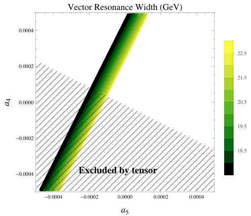


We would like to emphasize the very limited range of variation for the parameters that is shown in Figures 1 and 2. The constants and lay in the small region . (This region includes of course the MSM value , but —obviously— there are no resonances there.)
In order to convey a picture of the sort of predictive power of unitarization techniques we plot in Figure 3 the allowed bands in the broader range that was considered in a previous work [1] as still being phenomenologically acceptable. Indeed, setting even a relatively loose bound for the mass of the resonance restricts the range of variation of the relevant low-energy constants enormously. In the same Figure 3 we show a blown-up of the region where both a scalar and a vector resonance in this mass range may coexist. The dashed area is excluded as acceptable for effective EWSBS theories (see [3]).


III Experimental visibility of the resonances
The statistics so far available from the LHC experiments is limited. Searching for new particles in the LHC environment is extremely challenging and analyzing the contribution of possible resonances to an experimental signal is not easy without a well defined theoretical model with definite predictions for the couplings, form factors, etc. The IAM method is able not only of predicting resonance masses and widths but also their couplings to the . In [1, 3] the experimental signal of the different resonances was compared to that of a MSM Higgs with an identical mass. Because the decay modes are similar (in the vector boson channels that is) and limits on different Higgs masses are very documented this was a rather intuitive way of presenting the cross-section for possible EWSBS resonances, but it is not that useful for heavy resonances as the signal of an hypothetical Higgs of analogous mass becomes very broad and diluted. This point and several others were discussed in detail in [1]. Here we shall give very simple estimates of some cross-sections based on the Effective W Approximation (EWA) [24] in a couple of channels. These estimates should be taken as extremely tentative and only relevant to establish comparisons between different masses and channels. In the last section we will introduce form factors and vertex functions to allow for a proper comparison with experiment. Please note that in the amplitudes where scalars contribute the contribution of the 125 GeV Higgs is also included.
Some results for the cross sections are depicted in Figure 5 for the processes and . In the first case we quote the contribution from a possible vector resonance only (a scalar resonance is also possible in this process). In the second case only scalar exchange is possible. Note that both diboson production modes are sub-dominant at the LHC with respect to gluon production mediated by a top-quark loop and that the possible resonances in the scenario discussed here couple only to dibosons.
Compared to the preliminary experimental indications, the results quoted for the cross-sections of these two specific processes are low, particulary for vector resonances, but there are several caveats. First of all, the EWA tends to underestimate the cross-sections and it is difficult to assess its validity in the present kinematical situation. Second, in this region of parameter space the cross-sections do change very quickly with only small changes of the parameters thus adding an element of uncertainty. Finally, the quoted cross sections correspond to considering only the interval so as to have some intuition on the contribution of the resonance itself. It should also be mentioned that, as discussed in [1], there is an enhancement in the channel when both the vector and scalar resonances become nearly degenerate; this is possible in a limited region of parameter space. Also as previously stated, the scalar channel is enhanced if .
Interesting as partial waves for a given process may be, they are not that useful to implement unitarization in a Monte Carlo generator in order to make detailed quantitative comparison with experiment. One would need to implement diagrammatic and for that one needs vertex functions and propagators wherewith to construct and compute the contribution from different topologies. Our proposal to tackle this problem is presented next.
IV Introducing form factors
The amplitude will be denoted by . Using isospin and Bose symmetries this amplitude can be expressed in terms of a universal function as
| (5) |
with . The fixed-isospin amplitudes are given by the following combinations
| (6) | |||||
In writing these expressions we assume exact crossing symmetry 44 4 This remark is pertinent because amplitudes involving longitudinally polarized bosons are not crossing symmetric. The formulae can be easily extended to this case but become somewhat more involved and will not be reported here. See [1].. We also write the reciprocal relations (also assuming exact crossing symmetry)
| (7) | |||||
Other amplitudes (such as e.g. ) can be obtained trivially from the previous ones using obvious symmetries (and crossing symmetry too).
The partial wave amplitudes for fixed isospin and total angular momentum are defined by
| (8) |
where the are the Legendre polynomials and , with being the mass , and are the first non-vanishing partial waves in the present case. The poles in the respective unitarized partial wave amplitudes dictate the presence or absence of EWSBS resonances in the different channels.
We would like to express any amplitude as the sum of exchanges of resonances in the , and channels, as it is diagrammatically expressed in Figure 6. That is, we decompose, say
| (9) |
Not all receive contributions from all three channels. For example, in the case a possible scalar resonance only contributes to the -channel. In addition, not all processes are resonant in all regions of parameter space, so the above decomposition assumes resonance saturation.

Let us now define the vector form factor as55 5 CVC has been used.
| (10) |
where is the interpolating vector current with isospin index that creates the resonance and is the vector form factor. From this form factor we derive a vector vertex function via the relation
| (11) |
Let us focus for instance on the amplitude that has potentially contributions from a vector and a tensor. The IAM does exclude the contribution [3] so let us consider for this process. It can be expressed as
| (12) |
where . Analogous decompositions exist for and . In fact we do not need to consider and at all because assuming exact isospin symmetry . Here we assume, and it is a necessary ingredient of the present approach, that external lines are on-shell.
On the other hand from unitarization we know that
| (13) |
so neglecting further partial waves it is natural to identify
| (14) |
where for we can use the IAM approximation
| (15) |
Although should of course be real and positive, when using the identification above we get a tiny imaginary part () due to the fact that we are missing possible channels (including non-resonant contributions) and terms in the partial wave expansion. However we can regard the description of the amplitude via vertex functions and resonance propagators as quite satisfactory in the regions where resonances are present.
Neglecting the gauge boson mass (quite justified at 2 TeV) unitarity requires the form factor to obey the following relation within a vector dominance region [19]
| (16) |
Equation (16) allows us to extract the phase of . Thus, combining the phase and the modulus we obtain the vector form factor
| (17) |
Similar techniques could allow us to define a unitarized scalar form factor and a vertex function directly derived from the unitarized amplitude that in this channel is
| (18) |
and assuming resonance dominance. In Figure 7 we plot the vertex functions and obtained by the method just described:
| (19) |
Note that the function is dimensionless while has units of energy. However for vector resonances, the effective coupling is typically (see the expression for the form factor and the associated Feynman rule). In the last figure we plot these effective couplings normalized to the scale . The contribution to the form factor from the 125 GeV Higgs is negligible around the scalar resonance at TeV.
Once we feel confident that the combination of resonant propagators and the vertex functions just given reproduces very satisfactorily the unitarized amplitudes we can pass on this information to Monte Carlo generator practitioners to implement these form factors in their favorite generator.
The expressions for , and needed to reproduce the diagrammatic expansion for the various values of and , can be found in [1, 2, 3] (and [4, 6] if a full use of the equivalence theorem is made66 6 Please note that -channel exchange is not included in some of these works.). Further details will be provided in a forthcoming extended publication.
V Conclusions
To conclude, we have extracted the values of the low-energy constants and of the effective Lagrangian describing an extended electroweak symmetry breaking sector assuming (iso)vector dominance and/or (iso)scalar dominance with a mass in the range 1.8 TeV 2.2 TeV, as it would be the case if one considers the preliminary results coming from the LHC experiment to be a hint of the existence of new interactions. The calculation was performed in the framework of the inverse amplitude unitarization method. We derived the widths of such resonances, which turn out to be quite narrow. We also speculated on the possibility of more than one resonance being present compatible with the derived bounds on and (something that is favoured by custodial symmetry considerations). The given range of masses restrict enormously the admissible values for and —surely a consequence of this mass scale being relatively close to the natural cut-off of the effective theory ( TeV). The cross-sections obtained using the Effective W approximation are however two low, particularly for vector resonances, and this may eventually prove bad news for resonances of the kind considered here. However we regard estimates based on the EWA as being too preliminary at this point.
To overcome this difficulty we proposed a diagrammatic method to deal with resonances in regions of parameter space in the effective Lagrangian where the former are assumed to dominate. We derived the corresponding form factors and vertex functions. The agreement with the full amplitude is very good and we understand that the technique that we introduce here may be useful to deal with the type of resonances that may emerge in EWSBS. We hope that this will trigger interest from our experimental colleagues to incorporate this seemingly consistent unitary procedure in their generators to allow for a proper theory-experiment comparison. In fact having a reliable estimate of the resonances cross sections in the region of interest is probably the most urgent task.
The apparent signal coming from the LHC experiments has triggered a flurry of activity that has mostly concentrated in proposing specific models ranging from introducing resonances [25] to the obvious possibility of excited or left-right symmetric states to more exotic models [27]. Our proposal is somewhat different: it is not primarily aimed at advancing a definite ad hoc proposal but rather to help understand if the signal is there in the first place and at trying to elucidate the properties of the resonance (or resonances) that might be present in an extended electroweak symmetry breaking sector in scattering. We regard the restriction on some coefficients of the effective Lagrangian provided by unitarity considerations as non-trivial and, if confirmed, would undoubtedly play a relevant role in constraining the underlying model.
Acknowledgements
We thank R. Delgado, A. Dobado, F. Llanes-Estrada and J.R. Peláez for discussions concerning different aspects of unitarization and effective lagrangians. D.E. thanks the Perimeter Institute where this work was initiated for the hospitality extended to him. We acknowledge the financial support from projects FPA2013-46570, 2014-SGR-104 and CPAN (Consolider CSD2007-00042). Funding was also partially provided by the Spanish MINECO under project MDM-2014-0369 of ICCUB (Unidad de Excelencia ‘Maria de Maeztu’)
References
- [1] D. Espriu and B. Yencho, Phys. Rev. D 87, no. 5, 055017 (2013).
- [2] D. Espriu, F. Mescia and B. Yencho, Phys. Rev. D 88, 055002 (2013).
- [3] D. Espriu and F. Mescia, Phys.Rev. D 90, 015035 (2014).
- [4] R. Delgado, A. Dobado, and F. Llanes-Estrada, J.Phys. G 41, 025002 (2014); JHEP 1402, 121 (2014); Phys. Rev. Lett. 114, 221803 (2015).
- [5] D. Barducci, H. Cai, S. De Curtis, F. Llanes-Estrada and S. Moretti, Phys. Rev. D 91, 095013 (2015).
- [6] R. Delgado, A. Dobado and F. Llanes-Estrada, Phys.Rev. D 91, 075017 (2015).
- [7] T.N. Truong, Phys. Rev. Lett. 61 (1988) 2526; A. Dobado, M.J. Herrero and T.N. Truong, Phys.Lett. B235 (1990) 134; A. Dobado and J.R. Pelaez, Phys. Rev. D 47 (1993) 4883; Phys. Rev. D 56 (1997) 3057; J.A. Oller, E. Oset and J.R. Pelaez, Phys. Rev. Lett. 80 (1998) 3452; Phys. Rev. D 59 (1999) 0740001; 60 (1999) 099906(E); F. Guerrero and J.A. Oller, Nucl. Phys. B 537 (1999) 459; A. Dobado and J.R. Pelaez, Phys. Rev D 65 (2002) 077502; A. Filipuzzi, J. Portoles and P. Ruiz-Femenia, JHEP 1208, 080 (2012); PoS CD 12, 053 (2013).
- [8] A. Alboteanu, W. Kilian and J. Reuter, JHEP 0811 (2008) 010; W. Kilian, T. Ohl, J. Reuter and M. Sekulla, Phys.Rev. D91 (2015) 096007.
- [9] J.M. Cornwall, D.N. Levin and G.Tiktopoulos, Phys. Rev. D10 (1974) 1145; C. E. Vayonakis, Lett. Nuovo Cim. 17, 383 (1976).; B.W. Lee, C. Quigg and H. B. Thacker, Phys. Rev. D16 (1977) 1519; G.J. Gounaris, R. Kogerler and H. Neufeld, Phys. Rev. D34 (1986) 3257; M.S. Chanowitz and M.K. Gaillard, Nucl. Phys. B261 (1985) 379; A. Dobado and J.R. Pelaez, Nucl.Phys. B425 (1994) 110; Phys. Lett. B329 (1994) 469; C. Grosse-Knetter and I.Kuss, Z.Phys. C66 (1995) 95; H.J.He,Y.P.Kuang and X.Li, Phys. Lett. B329 (1994) 278.
- [10] D. Espriu and J. Matias, Phys. Rev. D 52 (1995) 6530.
- [11] A. Adams, N. Arkani-Hamed, S. Dubovsky, A. Nicolis and R. Rattazzi (CERN), JHEP 0610 (2006) 014.
- [12] C. Englert, P. Harris, M. Spannowsky and M. Takeuchi, Phys.Rev. D92 (2015) 1, 013003; G. Cacciapaglia and M. T. Frandsen, arXiv:1507.00900; T. Abe, R. Nagai, S. Okawa and M. Tanabashi, arXiv:1507.01185
- [13] G. Aad et al. [The ATLAS collaboration], arXiv:1506.00962.
- [14] V. Khachatryan et al. [The CMS collaboration], JHEP 1408 (2014) 173; R. Koegler, http://indico.cern.ch/event/388148/attachments/775833/.
- [15] B. C. Allanach, B. Gripaios and D. Sutherland, arXiv:1507.01638; J.A. Aguilar-Saavedra, arXiv:1506.06739
- [16] H. Georgi and M. Machacek, Nucl. Phys. B 262, 463 (1985).
- [17] A. Falkowski, S. Rychkov and A. Urbano, JHEP 1204 (2012) 073; A. Urbano, arXiv:1310.5733 [hep-ph].
- [18] A. Dobado, D. Espriu and M.J. Herrero, Phys.Lett. B255 (1991) 405; D. Espriu and M.J. Herrero, Nucl.Phys. B373 (1992) 117; M.J. Herrero and E. Ruiz-Morales, Nucl.Phys. B418 (1994) 431; Nucl. Phys. B 437 (1995) 319; D. Espriu and J. Matias, Phys.Lett. B341 (1995) 332; 1; R. Foadi, M. Jarvinen and F. Sannino, Phys. Rev. D 79, 035010 (2009).
- [19] A. Dobado, M.J. Herrero, J.R. Peláez and E. Ruiz-Morales, Phys. Rev. D 62 (2000) 0550.
- [20] G. F. Giudice, C. Grojean, A. Pomarol and R. Rattazzi, JHEP 0706, 045 (2007); G. Buchalla and O. Cata, JHEP 1207, 101 (2012); R. Contino, M. Ghezzi, C. Grojean, M. Muhlleitner and M. Spira, JHEP 1307, 035 (2013); R. Alonso, M. B. Gavela, L. Merlo, S. Rigolin and J. Yepes, Phys. Lett. B 722, 330 (2013); R. Alonso, I. Brivio, B. Gavela, L. Merlo and S. Rigolin, JHEP 1412, 034 (2014); G. Buchalla, O. Catà and C. Krause, Nucl. Phys. B 880, 552 (2014); G. Cacciapaglia and F. Sannino, JHEP 1404 (2014) 111.
- [21] A. Falkowski, F. Riva and A.Urbano, JHEP 1311, 111 (2013).
- [22] I. Brivio, T. Corbett, O. J. P. Eboli, M. B. Gavela, J. Gonzalez-Fraile, M. C. Gonzalez-Garcia, L. Merlo and S. Rigolin, JHEP 1403, 024 (2014).
- [23] A. Pich, I. Rosell, J.J. Sanz-Cillero, Phys.Rev.Lett. 110 (2013) 181801; A. Pich, I. Rosell and J.J. Sanz-Cillero, JHEP 1401 (2014) 157.
- [24] G. L. Kane, W. W. Repko and W. B. Rolnick, Phys. Lett. B 148, 367 (1984); S. Dawson, Phys. B 249, 42 (1985); M. S. Chanowitz and M. K. Gaillard, Nucl. Phys. B 261, 379 (1985).
- [25] H. S. Fukano, M. Kurachi, S. Matsuzaki, K. Terashi and K. Yamawaki, arXiv:1506.03751; D. B. Franzosi, M. T. Frandsen and F. Sannino, arXiv:1506.04392; A. Thamm, R. Torre and A. Wulzer, arXiv:1506.08688; T. Abe, T. Kitahara and M. M. Nojiri, arXiv:1507.01681; A. Carmona, A. Delgado, M. Quiros and J. Santiago, arXiv:1507.01914; C. W. Chiang, H. Fukuda, K. Harigaya, M. Ibe and T. T. Yanagida, arXiv:1507.02483; L. Bian, D. Liu, J. Shu, arXiv:1507.06018; M. Low, A. Tesi and L. T. Wang, arXiv:1507.07557.
- [26] J. Hisano, N. Nagata and Y. Omura, arXiv:1506.03931; K. Cheung, W.Y. Keung, P.Y. Tseng and T.C. Yuan, arXiv:1506.06064; Y. Gao, T. Ghosh, K. Sinha and J.H. Yu, arXiv:1506.07511; J.Yepes, arXiv:1507.03974; J. Yepes, R. Kunming and J Shu, arXiv:1507.04745.
- [27] A. Alves, A. Berlin, S. Profumo and F. S. Queiroz, arXiv:1506.06767; J. Brehmer, J. Hewett, J. Kopp, T. Rizzo and J. Tattersall, arXiv:1507.00013; Q. H. Cao, B. Yan and D. M. Zhang, arXiv:1507.00268; B. A. Dobrescu and Z. Liu, arXiv:1507.01923; G. Cacciapaglia, A. Deandrea and M. Hashimoto, arXiv:1507.03098; V. Sanz, arXiv:1507.03553; C. H. Chen and T. Nomura, arXiv:1507.04431; M. E. Krauss and W. Porod, arXiv:1507.04349; Y. Omura, K. Tobe and K. Tsumura, arXiv:1507.05028; W. Chao, arXiv:1507.05310; L. A. Anchordoqui, I. Antoniadis, H. Goldberg, X. Huang, D. Lust and T. R. Taylor, arXiv:1507.05299; D. Kim, K. Kong, H. M. Lee and S. C. Park, arXiv:1507.06312.