Swift: task-based hydrodynamics and gravity for cosmological simulations

Tom Theuns

Aidan Chalk

Matthieu Schaller Address: Institute for Computational Cosmology Address: Department of Physics Address: Durham University Address: Durham DH1 3LE, UK Address: School of Engineering and Computing Sciences Address: Durham University Address: Durham DH1 3LE, UK Address: Institute for Computational Cosmology Address: Department of Physics Address: Durham University Address: Durham DH1 3LE, UK Pedro Gonnet Address: School of Engineering and Computing Sciences Address: Durham University Address: Durham DH1 3LE, UK Address: and Address: Google Switzerland GmbH Address: Brandschenkestr. 110 Address: 8002 Zurich, Switzerland

29 July 2015

Abstract

Simulations of galaxy formation follow the gravitational and hydrodynamical interactions between gas, stars and dark matter through cosmic time. The huge dynamic range of such calculations severely limits strong scaling behaviour of the community codes in use, with load-imbalance, cache inefficiencies and poor vectorisation limiting performance. The new swift code exploits task-based parallelism designed for many-core compute nodes interacting via MPI using asynchronous communication to improve speed and scaling. A graph-based domain decomposition schedules interdependent tasks over available resources. Strong scaling tests on realistic particle distributions yield excellent parallel efficiency, and efficient cache usage provides a large speedup compared to current codes even on a single core. swift is designed to be easy to use by shielding the astronomer from computational details such as the construction of the tasks or MPI communication. The techniques and algorithms used in swift may benefit other computational physics areas as well, for example that of compressible hydrodynamics. For details of this open-source project, see www.swiftsim.com

keywords

Task-based parallelism, Asynchronous data transfer

1 Introduction

The main aim of cosmological simulations of the formation of structures in the Universe is to understand which physical processes play in role in how galaxies form and evolve. For example, what determines whether a galaxy becomes a spiral or an elliptical? What is the origin of the morphology-density relation - the observation that elliptical galaxies cluster much more strongly than spirals? What sets the colours of galaxies? How does the rate of galaxy formation evolve over cosmic time? What is the nature of high-redshift galaxies? A better understanding of these processes will be required to take full advantage of the rich data sets being collected now, or promised by future observatories such as the James Webb space telescope¹¹ 1 http://www.jwst.nasa.gov/, ESO’s Extremely-Large telescope ²² 2 http://www.eso.org/public/teles-instr/e-elt/ or the Square Kilometre Array ³³ 3 https://www.skatelescope.org/.

Such cosmological simulations start from initial conditions motivated by observations of the cosmic microwave background (CMB). The CMB provides a directly observable imprint of the small density fluctuations that will eventually grow due to gravity into galaxies and clusters of galaxies today. In an expanding universe, regions which are slightly over-dense become denser and eventually collapse due to the self-gravity of their dark matter. These collapsing ‘halos’ accrete gas that cools radiatively and makes stars. The simulations follow the build-up of the dark matter halos and the accretion, shock-heating, and radiative cooling of the gas onto halos.

The gas densities above which stars form are orders of magnitude higher than the typical density in a galaxy and this large dynamic range is one of the most challenging aspects of these computations. The radiation and winds of recently formed stars, and the energy injected by super nova explosions, strongly limit the rate at which a galaxy’s gas is turned into stars. As a result, only $\sim 17$ per cent of all gas in the Universe has been converted into stars to date [3]. The tremendous dynamic range in mass, length and time, between gas accreting onto a halo and turning into stars prevents simulations to model these crucial processes in detail. ‘Subgrid’ schemes are therefore used to model processes that cannot (yet) be resolved numerically, not unlike what is done in other multi-scale calculations such as for example weather or climate modelling. Limiting the impact of these subgrid models by actually resolving some of the underlying physics is a tremendously exciting and computationally demanding challenge for the exascale era.

Current cosmological simulations often take months to run on hundreds to many thousands of cores. For example the recent EAGLE simulation [11] took 45 days to run on 4000 cores of the Durham Data Centric Cluster, part of the DIRAC infrastructure⁴⁴ 4 http://www.stfc.ac.uk/1263.aspx, and the simulation suite used nearly 40M core hours on the curie machine using a prace⁵⁵ 5 http://www.prace-ri.eu/ allocation of computer time. Such long run times are currently limiting scientific progress.

This paper discusses the swift code that is designed to over-come some of the limitations of community codes widely used in cosmology, in particular improving load-balance, cache-usage, and vectorisation. It also intends to shield the astronomer who intends to implement and test subgrid schemes from the underlying computational details.

2 Cosmological gas dynamics

This section provides a brief overview of the equations being integrated. Calculations are performed in co-moving coordinates ${\bf x}$ say for position, related to physical coordinates ${\bf r}$ by the time-dependent scale factor $a(t)$ , ${\bf r}=a{\bf x}$ (see for example [10]), but we will ignoring these details here. Performing these calculations using a Lagrangian scheme where the fluid is represented by a set of particles that move with the fluid’s speed is very advantageous, because the flow speeds are very large due to the large (gravitational) motions of forming galaxies.

Smoothed particle hydrodynamics (SPH, [4, 9]) is such a Langrangian scheme in which values for fluid variables are interpolated from a disordered particle distribution using kernel interpolation. For example the density $\rho$ and pressure gradient $\nabla p$ at the location ${\bf r}_{i}$ of particle $i$ are computed with equations of the form

	$\displaystyle\rho({\bf r}_{i})$	$\displaystyle=$	$\displaystyle\sum_{j}m_{j}\,W({\|{\bf r_{i}}-{\bf r_{j}}\|\over h_{i}})\,,$		(1)
	$\displaystyle\nabla p({\bf r}_{i})$	$\displaystyle=$	$\displaystyle\sum m_{j}\left({p({\bf r}_{i})\over\rho({\bf r}_{i})^{2}}+{p({\bf r}_{j})\over\rho({\bf r}_{j})^{2}}\right)\nabla W({\|{\bf r_{i}}-{\bf r_{j}}\|\over h_{i}})$		(2)

where $m_{j}$ is the mass of particle $j$ and $W$ is a bell-shaped kernel with compact support, $W(q)=0$ for $q>1$ . The smoothing length $h_{i}$ is computed such that a given weighted number of particles contributes to the sum. The pressure is found from the density and temperature using an equation of state. Note that we need to evaluate the density for each particle before we can compute the pressure gradient. Several variations of Eq. (2) exist, we use this particular form here to illustrate the type of sums to be computed, swift implements the more accurate version used in gadget 2 [12].

Gravitational accelerations are calculated as,

{\bf a}_{i}=-{\rm G}\sum_{j\neq i}\,{m_{j}\over|{\bf r_{i}}-{\bf r_{j}}|^{3}}\,({\bf r}_{i}-{\bf r}_{j})\,,

(3)

with extra terms (not discussed here) to represent periodic images such that the simulated volume is periodically replicated (the Ewald summation familiar from solid state physics).

Given the initial state of the system, specified by position and velocities of all particles, particles are marched forward in time using velocities to update positions and accelerations to update velocities. Most of the calculation time is spent in evaluating the hydrodynamical and gravitational forces. The popular gadget [12] and gasoline [13] codes use a tree to find neighbours for evaluating the sum in Eqs. (1-2). These codes split the gravitational force from Eq. (3) into a contribution from nearby particles evaluated using a tree following [1], and contribution from distant particles evaluated using a mesh, as in the P3M scheme described in detail in [7], see [2] for the application in cosmology. The particles are distributed over the computational volume using a space-filling curve to attempt to preserve locality which reduces MPI communication needed if neighbour particles are not held on the same MPI task. Such ‘domain decomposition’ also takes significant compute time. How this issues are handled in swift is described next.

3 Task-based calculations

3.1 SPH

Refer to caption — Figure 1: Illustration of neighbour finding on a mesh. Five tasks are indicated, numbers 1-3 compute densities from pairs of particles in cells 1-3, whereas tasks 4 and 5 compute densities between particles pairs in neighbouring cells.

Swift identifies potential neighbours by organising particles in cubic cells as illustrated in Fig.1 (drawn in 1 dimension for simplicity). By choosing the cell size of the mesh to be larger than the smoothing length $h$ of all particles in that cell guarantees that particles within $h_{i}$ of the fat blue particle in the figure can be found either in the same cell (blue, labelled ‘2’), or in one of the two neighbouring cells (black and green, labelled ‘1’ and ‘3’ respectively). Given the large dynamic range in $h$ , such a mesh needs to be adaptive. The density calculation of Eq. (1) for particle $i$ now involves three steps: find neighbours of $i$ in each of the three cells (in the figure, these are particles within the red circle with radius $h_{i}$ ).

In Swift, each of these calculations is executed by separate tasks. In the simple case illustrated in Fig.1 there are two types: tasks that involve evaluating Eq. (1) for pairs of particles in the same cell (labelled 1-3), and tasks that involve evaluating Eq. (1) for pairs of particles in neighbouring cells (labelled 4 and 5). To avoid race conditions, some tasks cannot be performed simultaneously, in this particular case tasks 4 and 5 conflict will each other, 4 conflicts with 1 and 2, and 5 with 2 and 3 . The task scheduling in swift therefore should be able to handle both conflicts and dependencies.

How these 5 tasks could be executed by two threads is illustrated in Fig. 2. At the start, threads pick tasks independently, locking those tasks that conflict with them. In this example, thread 1 executes task 1, and thread 2 executes task 5 (locking tasks 2 and 3). When thread 2 completes task 5 it unlocks tasks 2 and 3, and starts executing task 3 (locking task 4). When task 3 is finished, thread 2 is idle because the remaining task 4 conflicts with task 2 being executed by thread 1. One of the threads (in the illustration thread 1) finishes off the work.

The efficiency of the tasks themselves can be improved by sorting [6, 5]. Indeed, consider again the fat blue particle $i$ in Fig.1 when task 5 is executed. If we were to sweep through the green particles in cell 3 from left to right, we would find that the fourth green particle no longer contributes to the density since it is outside the red circle. There is therefore no reason to even check if any of the other green particles is inside the red circle, since these are even further away from particle $i$ in the horizontal direction.

The swift SPH implementation contains several similar ‘kernels’ that calculate the interaction between two particles (for example individual terms in Eq. (1) or in Eq (2)). Exposing these basic routine to the user greatly simplifies adapting the code to the user’s wishes, for example in making changes to the basic SPH algorithm. This kernel is called for a range of particles that are in the same cell. Cache-misses are minimised by making sure these particles are nearly contiguous in memory. Bunching particles in cells is then also advantages for vectorising, either using intrinsics, or by using pragma’s that allow the compiler to known that these calculations can be vectorised.

With sorting tasks, density tasks, and pressure gradients tasks (and gravity tasks, described next) combined for all cells, a science run will typically contain hundreds or even millions of tasks. Individual threads on a many-core node can thus all be executing tasks as long as these do not conflict with each other, using task stealing to grab a new task as soon as their current task is completed. Once a thread grabs a new task, it blocks those tasks that conflict with it. In addition to conflicts, the swift task engine also handles task dependencies - for example the density of particles in a cell and its neighbouring cell should have been computed before pressure gradients can be computed.

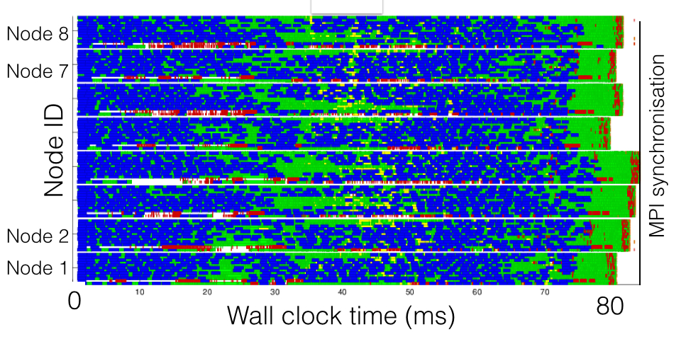
Running this task-based parallelisation across MPI tasks introduces relatively minimal additional complexity. If neighbouring cells are assigned to different MPI tasks, swift will generate extra communication tasks that exchange the contents of individual cells using asynchronous communication. The distribution of particles (or rather cells) across MPI tasks is based on the total costs of tasks - assigning similar work to each MPI task - while aiming to minimise communication that results from spatially non-contiguous particle distributions. Generating and scheduling the inter-dependent tasks is performed in a similar way as is done in the QuickSched library [5] using the metis library [8] to partition tasks over MPI tasks. An example is shown in Fig.3 (a realistic version of Fig. 2), which shows a time-line of how 8 nodes of 12 threads each execute a set of tasks using MPI across nodes. Running on a realistic particle distribution, swift achieves 60 per cent parallel efficiency in a strong scaling test increasing the core count from one to 1024 (see Fig. 4, see also [5]).

Using cells to organise particles spatially and identify potential neighbours may at first sight seem very different from using a tree as in the Gadget 2 or Gasoline codes. However the algorithms are actually surprisingly similar once one limits the depth of the tree to cells that contain $\sim 100$ particles as is the case in swift. How to find neighbouring cells in swift is actually also performed using a tree.

3.2 Gravity

Currently swift implements the Barnes-Hut tree code algorithm [1] for evaluating the gravitational acceleration from Eq. (3), with some modifications described below. The Barnes-Hut algorithm divides the simulation volume spatially and recursively in smaller cells. Such a division is very well suited for evaluating gravitational interactions. Indeed consider a particle $i$ at some distance from a tree node. A good approximation for the contribution of that node to ${\bf a}_{i}$ can be obtained using a multipole expansion, for example representing all the particles in the node by their monopole, as long as the distance particle-node is large compared to the extent of the node. If the distance is small, the node is split in its daughter cells, and the algorithm recurs.

This Barnes-Hut algorithm decreases the computational cost of evaluating ${\bf a}_{i}$ for all particles from order $N^{2}$ to order $N\log(N)$ [1]. Note that two particles that are spatially close are likely to execute nearly identical tree walks. In practise most of the compute time is now spent in the tree walk (rather than evaluating actual accelerations).

We implemented three optimisations of this algorithm in swift. Firstly we limit the depth of the tree from leaf nodes that contain a single particle (as in gadget) to cells with $\sim 100$ particles. This is because the tree walk is not very efficient for small numbers of particles.

Secondly we do not start a tree walk for each particle from the root node, but rather walk the tree walk for nodes. For each set of nodes, we decide whether they are sufficiently distant to compute forces using multipoles, or they should be split in their daughter nodes recursively. Doing so results in a list of tasks, those in which particles in one node interact with the multipole of another node, or those where all particles in one node interact with all particles in a nearby node. The latter task is implemented efficiently using the same task-based approach as used for SPH in the previous section.

Thirdly we use quadrupoles rather than monopoles. This increases time to solution minimally yet make the accelerations more accurate.

The speed and scaling of the tree implementation in swift is compared to that of gadget 2 in Fig. 5, in which ${\bf a}_{i}$ is calculated for each of 10M particles taken from the same snapshot of an eagle simulation as used in Fig. 4 (a very clustered distribution of particles). The speed of swift is close to that of gadget 2 when run on a single core, and the scaling up to 16 threads is close to ideal (parallel efficiency of 90 per cent). The public version of gadget 2 does not have multi-threading, and the scaling shown is when increasing the number of MPI tasks using one core per task.

4 Conclusions

We have implemented smoothed particle hydrodynamics (SPH) and a Barnes-Hut tree-code for self-gravity in the cosmological hydrodynamics code swift. By grouping nearby particles in cells, the calculation is broken-up into very many short and inter-dependent tasks, whereby a single task processes particles within a cell, or between pairs of cells. Task dependencies and conflicts are encoded in the application. Using cells improves cache efficiency and simplifies vectorisation. The tasks are distributed across nodes, with individual threads using task-stealing within a node, and communication being performed asynchronously between nodes. We find that such task-based parallelism is well suited to take advantage of the multiple levels of parallelism of modern many-core super computers. Applied to a realistic particle distribution, swift’s SPH implementation reaches a parallel efficiency of 60 per cent in a strong scaling test when increasing core count from 1 to 1024, and better than 90 per cent on a single 16-core node for gravity. Individual physics routines, for example those that evaluate interactions between two particles, are implemented in simple kernels to shield the physicist from the intricacies of tasks or MPI communications. swift is an open-source project, www.swiftsim.com.

Acknowledgments

This work used the DiRAC Data Centric system at Durham University, operated by the Institute for Computational Cosmology on behalf of the STFC DiRAC HPC Facility (www.dirac.ac.uk). This equipment was funded by BIS National E-infrastructure capital grant ST/K00042X/1, STFC capital grant ST/H008519/1, and STFC DiRAC Operations grant ST/K003267/1 and Durham University. DiRAC is part of the National E-Infrastructure. This work was supported by the Science and Technology Facilities Council [ST/F001166/1] and the European Research Council under the European Union’s ERC Grant agreements 267291 Cosmiway, by the Interuniversity Attraction Poles Programme initiated by the Belgian Science Policy ([AP P7/08 CHARM]), and by intel through establishment of the ICC as an intel parallel computing centre (IPCC).

References

[1] J. Barnes and P. Hut. A hierarchical O(N log N) force-calculation algorithm. Nature, 324:446–449, Dec. 1986.
[2] G. Efstathiou, M. Davis, S. D. M. White, and C. S. Frenk. Numerical techniques for large cosmological N-body simulations. ApJS, 57:241–260, Feb. 1985.
[3] M. Fukugita, C. J. Hogan, and P. J. E. Peebles. The Cosmic Baryon Budget. ApJ, 503:518–530, Aug. 1998.
[4] R. A. Gingold and J. J. Monaghan. On the fragmentation of differentially rotating clouds. MNRAS, 204:715–733, Aug. 1983.
[5] P. Gonnet. Efficient and Scalable Algorithms for Smoothed Particle Hydrodynamics on Hybrid Shared/Distributed-Memory Architectures. SIAM Journal on Scientific Computing, 37:95–121, Apr. 2015.
[6] P. Gonnet, M. Schaller, T. Theuns, and A. B. G. Chalk. SWIFT: Fast algorithms for multi-resolution SPH on multi-core architectures. ArXiv e-prints, Sept. 2013.
[7] R. W. Hockney and J. W. Eastwood. Computer simulation using particles. 1988.
[8] G. Karypis and V. Kumar. Fast and high quality multilevel scheme for partitioning irregular graphs. SIAM Journal on Scientific Computing, 20:359–392, 1998.
[9] L. B. Lucy. A numerical approach to the testing of the fission hypothesis. AJ, 82:1013–1024, Dec. 1977.
[10] P. J. E. Peebles. Principles of Physical Cosmology. 1993.
[11] J. Schaye, R. A. Crain, R. G. Bower, M. Furlong, M. Schaller, T. Theuns, C. Dalla Vecchia, C. S. Frenk, I. G. McCarthy, J. C. Helly, A. Jenkins, Y. M. Rosas-Guevara, S. D. M. White, M. Baes, C. M. Booth, P. Camps, J. F. Navarro, Y. Qu, A. Rahmati, T. Sawala, P. A. Thomas, and J. Trayford. The EAGLE project: simulating the evolution and assembly of galaxies and their environments. MNRAS, 446:521–554, Jan. 2015.
[12] V. Springel. The cosmological simulation code GADGET-2. MNRAS, 364:1105–1134, Dec. 2005.
[13] J. W. Wadsley, J. Stadel, and T. Quinn. Gasoline: a flexible, parallel implementation of TreeSPH. New A, 9:137–158, Feb. 2004.