Achieving proportional fairness with a control theoretic approach in error-prone 802.11e WLANsThanks: ¹ corresponding author S.H.Yang@lboro.ac.uk

We consider a single-hop 802.11e EDCA WLAN with one AP and $n$ client stations. Traffic flows are classified into $N$ ACs. We assume that each station only transmits traffic of a single AC, so no virtual collisions are considered in our analysis. The number of stations in the $i$th AC is $n_{i}$. Stations in the $i$th AC are assumed to have the same packet error rate $p_{i}$, and transmit packets at the same PHY data rate $r_{i}$. The packet size of all ACs is $L$ bits.

We start with the analysis of station throughput under saturated network loads. The following parameters are defined for AC $i$:

• •

  $CW_{min}^{i}$ is the minimum contention window;

• •

  $CW_{max}^{i}$ is the maximum contention window;

• •

  $AIFS_{i}$ is the duration of the Arbitration Inter-Frame Space, i.e. $AIFS_{i}=SIFS+t_{i}\times\sigma$, in which $t_{i}$ is the number of included time slots, $SIFS$ is the duration of the Short Inter-Frame Space and $\sigma$ is the duration of a physical time slot;

• •

  $M_{i}$ is the number of packets contained in a TXOP burst.

Due to the use of TXOP bursting, the RTS/CTS exchange mechanism is used to make fast recovery from collisions. If any packet within the TXOP burst fails due to channel errors, the burst is terminated and the station contends again for the channel to retransmit the failed packet. Therefore, a MAC time slot may be a PHY idle slot, a TXOP transmission or a RTS/CTS transmission.

Let $\tau_{i}$ denote the probability that a station in AC $i$ attempts to transmit in a time slot, and $\bm{\tau}=\{\tau_{i},\ i=0,\cdots,N-1\}$. The station throughput of AC $i$ is given by

in which $P^{I}=\prod\limits_{i=0}^{N-1}(1-\tau_{i})^{n_{i}}$ is the probability of an idle time slot and $P_{i}^{T}=\tau_{i}(1-\tau_{i})^{n_{i}-1}\prod\limits_{j=0,j\neq i}^{N-1}(1-\tau_{j})^{n_{j}}$ is the probability that a station of AC $i$ makes a TXOP transmission. $T^{col}=T_{RTS}+EIFS$ is the duration of a collision, where $EIFS$ is the duration of the Extended Inter-Frame Space, which is given by $EIFS=T_{ACK}+SIFS+DIFS$. $\mathbb{E}(T_{i}^{txop})$ is the expected duration of a TXOP transmission from a station of AC $i$,

where $T^{oo}=T_{PHYhdr}+2SIFS+T_{ACK}$ is the protocol overheads associated with a single packet transmission within a TXOP burst, and $T_{i}^{o}=T_{RTS}+SIFS+T_{CTS}+AIFS_{i}$ is the protocol overheads associated with the transmission of the burst. $\mathbb{E}(Pld_{i}^{txop})$ is the expected payload transmitted in a TXOP burst of AC $i$,

Next, we will calculate the average packet transmission delay. As the delay is mainly dominated by the number of retransmission attempts caused by either collisions or erroneous transmissions, we ignore the countdown and blocking delays considered in [1]. The average delay of a TXOP burst consists of the following two expected delays:

• •

  Expected collision delay: Assuming that $m$ is the retry limit and $CW_{max}^{i}=2^{m}{CW}_{min}^{i}$, the expected collision delay is

  $$D_{i}^{col}=T^{col}\bigg(\sum\limits_{j=1}^{m}j\big(P_{i}^{C}\big)^{j}\big(1-P_{i}^{C}\big)+(m+1)\big(P_{i}^{C}\big)^{m+1}\bigg)$$

  in which $P_{i}^{C}$ is the conditional collision probability,

  $$P_{i}^{C}=1-(1-\tau_{i})^{n_{i}-1}\prod\limits_{\begin{subarray}{c}j=0,j\neq i\end{subarray}}^{N-1}(1-\tau_{j})^{n_{j}}$$

• •

  Expected TXOP transmission delay: The expected TXOP transmission delay is calculated by multiplying the expected number of transmissions by the expected duration of a TXOP burst.

  $$\begin{split}D_{i}^{txop}=&\mathbb{E}({T}_{i}^{txop})\bigg(\sum\limits_{j=1}^{m+1}j\big(1-P_{i}^{C}\big)^{j}\big(P_{i}^{E}\big)^{j-1}\big(1-P_{i}^{E}\big)\\ &+(m+1)\big(1-P_{i}^{C}\big)^{m+1}\big(P_{i}^{E}\big)^{m+1}\bigg)\end{split}$$

  in which $P_{i}^{E}=1-(1-p_{i})^{M_{i}}$ is the probability of a TXOP failure due to channel noise.

Combining the above two delays, the average delay of a single packet within a TXOP burst is therefore given by

The station throughput and average delay derived above are functions of station attempt probabilities. Next we will derive the relationship between $\tau_{i}$ and ${CW_{min}^{i}}$ based on the throughput model proposed in [2] but consider error-prone channels. The probability that a transmission fails due to either collisions or channel noise is given by

The probability that the backoff counter is suspended due to a busy channel during the period of $AIFS_{i}$ is

in which $t_{min}$ is the minimum $t$ value among all ACs. The relationship between $\tau_{i}$ and $CW_{min}^{i}$ is then given by

In this section we aim at finding the optimal $\bm{\tau}$ to achieve proportional fair allocation of station throughputs given distinct average delay constraints for different ACs.

The adaptive control algorithm is performed centrally at the AP every beacon interval, which is typically 100ms in 802.11 WLANs, and consists of two steps:

1. 1.

   At the end of each beacon interval, the observed failure probability $\bm{p^{F}}$ resulting from the current $\bm{CW_{min}}$ is measured by the AP.

2. 2.

   The controller computes a new set of $\bm{CW_{min}}$ based on the measured $\bm{p^{F}}$. An update of $\bm{CW_{min}}$ is then distributed to the WLAN by the next beacon frame.

As the period of the adaptive control algorithm is long enough to assume that the measurement corresponds to stationary conditions, i.e. the system has no memory, $\bm{p^{F}}$ depends only on the current $\bm{CW_{min}}$. Eqn. (3) and Eqn. (4) give a non-linear relationship between $\bm{p^{F}}$ and $\bm{CW_{min}}$. To simplify the controller design, we will use a linear approximation to this non-linear relationship around the stable point of operation,

in which

With the linearisation, the WLAN can be represented as a discrete MIMO state-space model. The failure probability at instant $k+1$ is determined by the minimum contention window input to the WLAN at instant $k$, the state and measurement equations are therefore given by

in which the system state is $\bm{x}(k)=[\bm{p^{F}}(k)]^{T}$; the system input is $\bm{u}(k)=[\bm{CW_{min}}(k)]^{T}$; the system model matrices are $\bm{B}=-\bm{H}^{T}$ and $\bm{C}=\bm{I}_{N\times N}$; the system output is $\bm{y}(k)=\bm{C}\bm{x}(k)=[\bm{p^{F}}(k)]^{T}$.

The control task can be accomplished by using the LQI control method  [3] to design our controller. Fig. 1 shows the control block diagram for the system, in which the controller input ${r}(k)={p^{F}}^{*}$ is the optimal failure probability, $e(k)=r(k)-y(k)$ is the error between the output feedback and the input reference value, and ${s}(k)={s}(k-1)+T_{s}e(k-1)$ is the output of a discrete integrator and $T_{s}$ is the sampling period. The $\bm{K}\in\mathbb{R}^{N\times 2N}$ is the control gain matrix.

The LQI controller computes an optimal state-feedback control law

by minimising the quadratic cost function

for any initial state $\bm{x}(0)$, in which $\bm{z}(k)=[\bm{x}(k);\bm{s}(k)]$. The optimal state feedback gain matrix $\bm{K}$ is computed by solving the associated discrete algebraic Riccati equation [3].

The matrices $\bm{Q}$ and $\bm{R}$ are the weighting matrices respectively indicating the state and control cost penalties. $\bm{Q}$ and $\bm{R}$ are required to be real symmetric and positive definite. The selection of weighting matrices $\bm{Q}$ and $\bm{R}$ affect the convergence speed of the controller.

We will first evaluate the impact of packet error rates on the station throughput and delay performances. Consider a WLAN with four stations and each station transmits a traffic flow of a distinct AC. The protocol parameter values used in the simulations are listed in Table I. Fig. 2 plots the throughput, average delay and station attempt probability of four ACs as the packet error rate $p_{VI}$ varies while keeping $p_{BE}=p_{VO}=p_{BK}=10^{-6}$. It can be seen that as the PER increases, the station in AC$\_$VI attempts harder with an increasing attempt probability but the throughput and delay performances irreversibly degrade. The increase of $p_{VI}$ also results in the decrease of attempt probabilities of the other three ACs, but the coupling of station transmissions lead to invariant delay and throughput performances, which implies that the delay and throughput of an AC are only dependent on its own PER.

The flow total air-time is defined as the fraction of time used for transmitting a flow. For a flow of AC $i$, the flow total air-time consists of the successful flow air-time and the collision air-time, given by

Again we consider a WLAN with four stations individually carrying a flow of a distinct AC. Fig. 3(a) plots the flow total air-times of four ACs as the delay deadline of AC$\_$VO varies while keeping that of the other three ACs fixed. It can be seen that when $d_{VO}\leq 210$ms, the delay constraint of AC$\_$VO keeps tight, and four flows have different air-times. As $d_{VO}$ increases, the air-time allocation is getting more and more even. When $d_{VO}$ increases up to 210ms, the four flow total air-times are equalised and all the delay constraints become loose now. Fig. 3(b) plots the sum of flow total air-times. We find that if any of the imposed delay constraints is tight, the air-times sum is larger than 1, otherwise they sum to unity. As the delay deadline is increased, the sum of collision air-times is decreasing while the sum of successful air-times is increasing. The fact that the air-times sum is not less than 1 is reasonable as the flow air-time usage overlaps due to collisions. This does not imply that the channel idle probability $P^{idle}=0$.

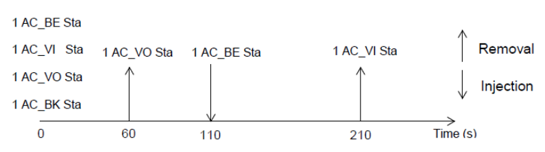
We will next evaluate the adaptivity of the proposed control method to changes in the network size. The example is depicted in Fig. 4. Four stations, one in each AC, join the network at $t=0$s. The station in AC$\_$VO leaves at t = 60s. One more station in AC$\_$BE joins the network at $t=110$s, and the station in AC$\_$VI leaves at $t=210$s. Fig. 5 plots the variation of $CW_{min}$ and the station throughput over time. The selection of matrices Q and R uses the trial and error method. It can be seen that $CW_{min}$ converges to the desirable value very quickly when the network size changes as long as proper Q and R are chosen. Moreover, the steady-state errors can be neglected, which means the control system has high accuracy performance.

References

- [1] X. Chen, I. Akinyemi and S. Yang, “A control theoretic approach to achieve proportional fairness in 802.11e EDCA WLANs”, accepted by Computer Communications, 2015.
- [2] K. Kosek-Szott, M. Natkaniec and A. R. Pach, “A simple but accurate throughput model for IEEE 802.11 EDCA in saturation and non-saturation conditions”, Computer Networks, 55(3), pp. 622-635, 2011.
- [3] P. C. Young and J. C. Willems, “An approach to the linear multivariable servomechanism problem”, International Journal of Control, 15(5), pp. 961-979, 1972.
- [4] D. P. Bertsekas, A. Nedich and A. E. Ozdaglar, Convex Analysis and Optimization. Athena Scientific, Belmont, MA, 2003.