Beyond Low Rank + Sparse:
Multi-scale Low Rank Matrix DecompositionF. Ong and M. Lustig are with the Department of Electrical Engineering and Computer Sciences, University of California, Berkeley, CA 94709 USA (e-mail: frankong@berkeley.edu and mlustig@eecs.berkeley.edu). This work is supported by NIH grants R01EB019241, R01EB009690, and
P41RR09784, Sloan research fellowship, Okawa research grant and NSF GRFP.
Abstract
We present a natural generalization of the recent low rank + sparse matrix decomposition and consider the decomposition of matrices into components of multiple scales. Such decomposition is well motivated in practice as data matrices often exhibit local correlations in multiple scales. Concretely, we propose a multi-scale low rank modeling that represents a data matrix as a sum of block-wise low rank matrices with increasing scales of block sizes. We then consider the inverse problem of decomposing the data matrix into its multi-scale low rank components and approach the problem via a convex formulation. Theoretically, we show that under various incoherence conditions, the convex program recovers the multi-scale low rank components either exactly or approximately. Practically, we provide guidance on selecting the regularization parameters and incorporate cycle spinning to reduce blocking artifacts. Experimentally, we show that the multi-scale low rank decomposition provides a more intuitive decomposition than conventional low rank methods and demonstrate its effectiveness in four applications, including illumination normalization for face images, motion separation for surveillance videos, multi-scale modeling of the dynamic contrast enhanced magnetic resonance imaging and collaborative filtering exploiting age information.
Index Terms:
Multi-scale Modeling, Low Rank Modeling, Convex Relaxation, Structured Matrix, Signal DecompositionI Introduction
Signals and systems often exhibit different structures at different scales. Such multi-scale structure has inspired a wide variety of multi-scale signal transforms, such as wavelets [Mallat:1989be], curvelets [Candes:2006bs] and multi-scale pyramids [Simoncelli:1992fh], that can represent natural signals compactly. Moreover, their ability to compress signal information into a few significant coefficients has made multi-scale signal transforms valuable beyond compression and are now commonly used in signal reconstruction applications, including denoising [Donoho:2006el], compressed sensing [Donoho:2006ci, Candes:2006eq], and signal separation [Donoho:2001hn, Starck:2005be, Chen:2006hm]. By now, multi-scale modeling is associated with many success stories in engineering applications.
On the other hand, low rank methods are commonly used instead when the signal subspace needs to be estimated as well. In particular, low rank methods have seen great success in applications, such as biomedical imaging [Liang:2007gf], face recognition [Basri:2003ie] and collaborative filtering [Goldberg:2001hj], that require exploiting the global data correlation to recover the signal subspace and compactly represent the signal at the same time. Recent convex relaxation techniques [Fazel:2002tc] have further enabled low rank model to be adaptable to various signal processing tasks, including matrix completion [Candes:2009kj], system identification [Fazel:2013dc] and phase retrieval [Candes:2013ka], making low rank methods ever more attractive.
In this paper, we present a multi-scale low rank matrix decomposition method that incorporates multi-scale structures with low rank methods. The additional multi-scale structure allows us to obtain a more accurate and compact signal representation than conventional low rank methods whenever the signal exhibits multi-scale structures (see Figure 1). To capture data correlation at multiple scales, we model our data matrix as a sum of block-wise low rank matrices with increasing scales of block sizes (more detail in Section II) and consider the inverse problem of decomposing the matrix into its multi-scale components. Since we do not assume an explicit basis model, multi-scale low rank decomposition also prevents modeling errors or basis mismatch that are commonly seen with multi-scale signal transforms. In short, our proposed multi-scale low rank decomposition inherits the merits from both multi-scale modeling and low rank matrix decomposition.

Leveraging recent convex relaxation techniques, we propose a convex formulation to perform the multi-scale low rank matrix decomposition. We provide a theoretical analysis in Section V that extends the rank-sparsity incoherence results in Chandrasekaran et al. [Anonymous:2011kn]. We show that the proposed convex program decomposes the data matrix into its multi-scale components exactly under a deterministic incoherence condition. In addition, in Section VI, we provide a theoretical analysis on approximate multi-scale low rank matrix decomposition in the presence of additive noise that extends the work of Agarwal et al. [Agarwal:2012gc].
A major component of this paper is to introduce the proposed multi-scale low rank decomposition with emphasis on its practical performance and applications. We provide practical guidance on choosing regularization parameters for the convex method in Section IV and describe heuristics to perform cycle spinning [Coifman:1995ji] to reduce blocking artifacts in Section IX. In addition, we applied the multi-scale low rank decomposition on real datasets and considered four applications of the multi-scale low rank decomposition: illumination normalization for face images, motion separation for surveillance videos, compact modeling of the dynamic contrast enhanced magnetic resonance imaging and collaborative filtering exploiting age information. (See Section X for more detail). Our results show that the proposed multi-scale low rank decomposition provides intuitive multi-scale decomposition and compact signal representation for a wide range of applications.
Related work
Our proposed multi-scale low rank matrix decomposition draws many inspirations from recent developments in rank minimization [Fazel:2002tc, Recht:2010dx, Agarwal:2012gc, Xu:2010uc, Candes:2010jb, Candes:2009kj, Recht:2010ht, Hsu:2011di]. In particular, the multi-scale low rank matrix decomposition is a generalization of the low rank + sparse decomposition proposed by Chandrasekaran et al. [Anonymous:2011kn] and Candès et al. [Candes:2011bd]. Our multi-scale low rank convex formulation also fits into the convex demixing framework proposed by McCoy et al. [McCoy:2013vc, McCoy:2014ir, McCoy:ky], who studied the problem of demixing components via convex optimization. The proposed multi-scale low rank decomposition can be viewed as a concrete and practical example of the convex demixing problem. However, their theoretical analysis assumes that each component is randomly oriented with respect to each other, and does not apply to our setting, where we observe the direct summation of the components. Bakshi et al. [Bakshi:1998il] proposed a multi-scale principal component analysis by applying principal component analysis on wavelet transformed signals, but such method implicitly constrains the signal to lie on a predefined wavelet subspace. Various multi-resolution matrix factorization techniques [Kondor:2014vr, Kakarala:2001fk] were proposed to greedily peel off components of each scale by recursively applying matrix factorization. One disadvantage of these factorization methods is that it is not straightforward to incorporate them with other reconstruction problems as models. Similar multi-scale modeling using demographic information was also used in collaborative filtering described in Vozalis and Margaritis [VOZALIS:2007ki].
II Multi-scale Low Rank Matrix Modeling

In this section, we describe the proposed multi-scale low rank matrix modeling in detail. To concretely formulate the model, we assume that we can partition the data matrix of interest into different scales. Specifically, we assume that we are given a multi-scale partition
Part I _
i }_i=1^ L M ×Nb
Part II _
i
Part III _
i-1R_b(X)bXm_i ×n_iM ×NYM ×NY ∑_i=1^ L X_i X_iP_iU_b,S_bV_bm_i ×r_b,r_b ×r_bn_i ×r_br_bR_b( X_i )R_b( X_i ) {U_b, S_b, V_b}X_i21 ×1M ×NYY { X_i }_i=1^ L X_i
II-A Multi-scale low rank + noise
Before moving to the convex formulation, we note that our multi-scale matrix modeling can easily account for data matrices that are corrupted by additive white Gaussian noise. Under the multi-scale low rank modeling, we can think of the additive noise matrix as the largest scale signal component and is unstructured in any local scales. Specifically if we observe instead the following
| (1) |
where is an independent and identically distributed Gaussian noise matrix. Then we can define a reshape operator that reshapes the entire matrix into an vector and the resulting matrix fits exactly to our multi-scale low rank model with scales. This incorporation of noise makes our model flexible in that it automatically provides a corresponding convex relaxation, a regularization parameter for the noise matrix and allows us to utilize the same iterative algorithm to solve for the noise matrix. Figure 5 provides an example of the noisy multi-scale low rank matrix decomposition.

III Problem Formulation and Convex Relaxation
Given a data matrix that fits the multi-scale low rank model, our goal is to recover the underlying multi-scale components using the fact that is block-wise low rank. Ideally, we would like to obtain a multi-scale decomposition with the minimal block matrix rank and solve a problem similar to the following form:
However, each rank minimization for each block is combinatorial in nature. In addition, it is not obvious whether the direct summation of ranks is a correct formulation as a -sparse matrix and a rank- matrix should intuitively not carry the same cost. Hence, the above non-convex problem is not a practical formulation to obtain the multi-scale decomposition.
Recent development in convex relaxations suggests that rank minimization problems can often be relaxed to a convex program via nuclear norm relaxation [Fazel:2002tc, Recht:2010ht], while still recovering the optimal solution to the original problem. In particular, Chandrasekaren et al. [Anonymous:2011kn] and Candès et al., [Candes:2011bd] showed that a low rank + sparse decomposition can be relaxed to a convex program by minimizing a nuclear norm + -norm objective as long as the signal constituents are incoherent with respect to each other. In addition, Candès et al., [Candes:2011bd] showed that the regularization parameters for sparsity and low rank should be related by the square root of the matrix size. Hence, there is hope that, along the same line, we can perform the multi-scale low rank decomposition exactly via a convex formulation.
Concretely, let us define to be the nuclear norm, the sum of singular values, and be the maximum singular value norm. For each scale , we consider the block-wise nuclear norm to be the convex surrogate for the block-wise ranks and define the block-wise nuclear norm for the th scale as
Its associated dual norm is then given by
which is the maximum of all block-wise maximum singular values.
We then consider the following convex relaxation for our multi-scale low rank decomposition problem:
| (2) | ||||||
where are the regularization parameters and their selection will be described in detail in section IV.
Our convex formulation is a natural generalization of the low rank + sparse convex formulation [Anonymous:2011kn, Candes:2011bd]. With the two sided matrix partition (Fig. 2), the nuclear norm applied to the blocks becomes the element-wise -norm and the norm for the largest scale is the nuclear norm. With the one sided matrix partition (Fig. ), the nuclear norm applied to blocks becomes the group-sparse norm and can be seen as a generalization of the group sparse + low rank decomposition [Xu:2010uc]. If we incorporate additive Gaussian noise in our model as described in Section II-A, then we have a nuclear norm applied to an vector, which is equivalent to the Frobenius norm.
One should hope that the theoretical conditions from low rank + sparse can be generalized rather seamlessly to the multi-scale counterpart. Indeed, in Section V, we show that the core theoretical guarantees in the work of Chandrasekaren et al. [Anonymous:2011kn] on exact low rank + sparse decomposition can be generalized to the multi-scale setting. In section VI, we show that the core theoretical guarantees in the work of Agarwal et al. [Agarwal:2012gc] on noisy matrix decomposition can be generalized to the multi-scale setting as well to provide approximate decomposition guarentees.
IV Guidance on Choosing Regularization Parameters
In this section, we provide practical guidance on selecting the regularization parameters . Selecting the regularization parameters is crucial for the convex decomposition to succeed, both theoretically and practically. While theoretically we can establish criteria on selecting the regularization parameters (see Section V and VI), such parameters are not straightforward to calculate in practice as it requires properties of the signal components before the decomposition.
To select the regularization parameters in practice, we follow the suggestions from Wright et al. [Anonymous:2013fx] and Fogel et al. [Foygel:cl], and set each regularization parameter to be the Gaussian complexity of each norm , which is defined as the expectation of the dual norm of random Gaussian matrix:
| (3) |
where denotes equality up to some constant and is a unit-variance independent and identically distributed random Gaussian matrix.
The resulting expression for the Gaussian complexity is the maximum singular value of a random Gaussian matrix, which has been studied extensively by Bandeira and Handel [Bandeira:2014wk]. The recommended regularization parameter for scale is given by
| (4) |
For the sparse matrix scale with block size, and for the globally low rank scale with block size, . Hence this regularization parameter selection is consistent with the ones recommended for low rank + sparse decomposition by Candès et al. [Candes:2011bd], up to a factor. In addition, for the noise matrix with block size, , which has similar scaling as in square root LASSO [Belloni:2011wd]. In practice, we found that the suggested regularization parameter selection allows exact multi-scale decomposition when the signal model is matched (for example Figure 1) and provides visually intuitive decomposition for real datasets.
For approximate multi-scale low rank decomposition in the presence of additive noise, some form of theoretical guarantees for the regularization selection can be found in our analysis in Section VI. In particular, we show that if the regularization parameters is larger than the Gaussian complexity of in addition to some “spikiness" parameters, then the error between recovered decomposition and the ground truth is bounded by the block-wise matrix rank.
V Theoretical Analysis for Exact Decomposition
In this section, we provide a theoretical analysis of the proposed convex formulation and show that if satisfies a deterministic incoherence condition, then the proposed convex formulation (2) recovers from exactly.
Our analysis follows similar arguments taken by Chandrasekaren et al. [Anonymous:2011kn] on low rank + sparse decomposition and generalizes them to the proposed multi-scale low rank decomposition. Before showing our main result (Theorem V.1), we first describe the subgradients of our objective function (Section V-A) and define a coherence parameter in terms of the block-wise row and column spaces (Section V-B).
V-A Subdifferentials of the block-wise nuclear norms
To characterize the optimality of our convex problem, we first look at the subgradients of our objective function. We recall that for any matrix with as its reduced SVD representation, the subdifferential of at is given by [Recht:2010ht, Watson:1992gq],
Now recall that we define the block-wise nuclear norm to be . Then using the chain rule and the fact that , we obtain an expression for the subdifferential of at as follows:
To simplify our notation, we define and to be a vector space that contains matrices with the same block-wise row spaces or column spaces as , that is,
where is the size of the block matrices for scale and is the matrix rank for block . Then, the subdifferential of each at can be compactly represented as,
We note that can be thought of as the “sign" of the matrix , pointing toward the principal components, and, in the case of the sparse scale, is exactly the sign of the entries.
In the rest of the section, we will be interested in projecting a matrix onto , which can be performed with the following operation:
Similarly, to project a matrix onto the orthogonal complement of , we can apply the following operation:
where is an appropriately sized identity matrix.
V-B Incoherence
Following Chandrasekaren et al. [Anonymous:2011kn], we consider a deterministic measure of incoherence through the block-wise column and row spaces of . Concretely, we define the coherence parameter for the th scale signal component with respect to the th scale to be the following:
| (5) |
Using as a measure of incoherence, we can quantitatively say that the th scale signal component is incoherent with respect to the th scale if is small. In the case of low rank + sparse, Chandrasekaren et al. [Anonymous:2011kn] provides excellent description of the concepts behind the coherence parameters. We refer the reader to their paper for more detail.
V-C Main Result
Given the above definition of incoherence, the following theorem states our main result for exact multi-scale low rank decomposition:
Theorem V.1.
If we can choose regularization parameters such that
then is the unique optimizer of the proposed convex problem (2).
In particular when the number of scales , the condition on reduces to and the condition on reduces to , which is in similar form as Theorem 2 in Chandrasekaren et al. [Anonymous:2011kn].
The proof for the above theorem is given in Appendix A.
VI Theoretical Analysis for Approximate Decomposition
In this section, we provide a theoretical analysis for approximate multi-scale low rank decomposition when the measurement is corrupted by additive noise as described in Section II-A. Our result follows arguments from Agarwal et al. [Agarwal:2012gc] on noisy -scale matrix decomposition and extends it to the multi-scale setting.
Instead of using the incoherence parameter defined for the exact decomposition analysis in Section V, we opt for a weaker characterization of incoherence between scales for approximate decomposition, studied in Agarwal et al. [Agarwal:2012gc]. Concretely, we consider spikiness parameters between the th signal component and th scale norm such that,
for each . Hence, if is small, we say is not spiky with respect to the th norm.
For analysis purpose, we also impose the constraints in the convex program. That is, we consider the solution from the following convex program:
| (6) | ||||||
| subject to | ||||||
| (7) | ||||||
We emphasize that the additional constraints (7) are imposed only for the purpose of theoretical analysis and are not imposed in our experimental results. In particular, for our simulation example in Figure 5, the minimizer of the convex program (2), using the recommended regularization parameters in Section IV, satisfied the constraints (7) even when the constraints were not imposed.
Let us define and to be the errors between the ground truth components and and the minimizers of convex program (6). Then, equivalently, we can denote and as the minimizers of the convex program (6). The following theorem states our main result for approximate decomposition.
Theorem VI.1.
If we choose such that
| (8) |
and such that
| (9) |
then the error is bounded by
where denotes inequality up to a universal constant.
Hence, when the spikiness parameters are negligible and , where is an independent, identically distributed Gaussian noise matrix with unit variance and is the noise standard deviation, choosing and ensures the condition is satisfied with high probability. This motivates the recommended regularization selection in Section IV.
The proof for the above theorem is given in Appendix B and follows arguments from Agarwal et al. [Agarwal:2012gc] on noisy matrix decomposition and Belloni et al. [Belloni:2011wd] on square root LASSO.
VII An Iterative Algorithm for Solving the Multi-scale Low Rank Decomposition
In the following, we will derive an iterative algorithm that solves for the multi-scale low rank decomposition via the Alternating Direction of Multiple Multipliers (ADMM) [Boyd:2011bw]. While the proposed convex formulation (2) can be formulated into a semi-definite program, first-order iterative methods are commonly used when solving for large datasets for their computational efficiency and scalability. A conceptual illustration of the algorithm is shown in Figure 6.
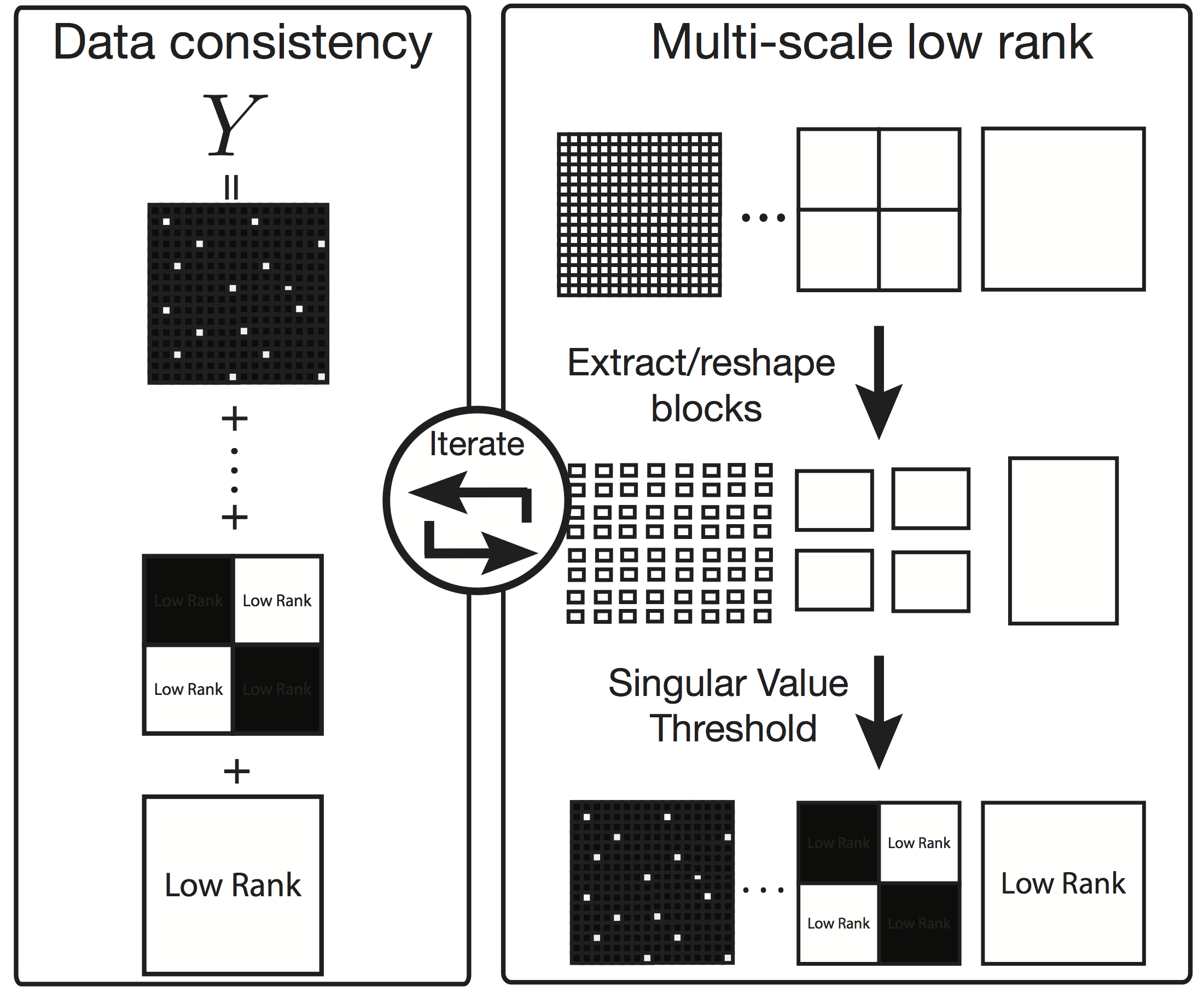
To formally obtain update steps using ADMM, we first formulate the problem into the standard ADMM form with two separable objectives connected by an equality constraint,
| (10) | ||||||
where is the indicator function.
To proceed, we then need to obtain the proximal operators [Parikh:2013vb] for the two objective functions and . For the data consistency objective , the proximal operator is simply the projection operator to the set. To obtain the proximal operator for the multi-scale nuclear norm objective , we first recall that the proximal operator for the nuclear norm with parameter is given by the singular value soft-threshold operator [Recht:2010ht],
| (11) |
Since we defined the block-wise nuclear norm for each scale as , the norm is separable with respect to each block and its proximal function with parameter is given by the block-wise singular value soft-threshold operator,
| (12) |
which simply extracts every blocks in the matrix, performs singular value thresholding and puts the blocks back to the matrix. We note that for blocks, the block-wise singular value soft-threshold operator reduces to the element-wise soft-threshold operator and for blocks, the block-wise singular soft-threshold operator reduces to the joint soft-threshold operator.
Putting everything together and invoking the ADMM recipe [Boyd:2011bw], we have the following algorithm to solve our convex multi-scale low rank decomposition (2):
| (13) |
where is the ADMM parameter that only affects the convergence rate of the algorithm.
The resulting ADMM update steps are similar in essence to the intuitive update steps in Figure 6, and alternates between data consistency and enforcing multi-scale low rank. The major difference of ADMM is that it adds a dual update step with , which bridges the two objectives and ensures the convergence to the optimal solution. Under the guarantees of ADMM, in the limit of iterations, and converge to the optimal solution of the convex program (2) and converges to a scaled version of the dual variable. In practice, we found that iterations are sufficient without any visible change for imaging applications. Finally, we note that because the proximal operator for the multi-scale nuclear norm is computationally simple, other proximal operator based algorithms [Parikh:2013vb] can also be used.
VIII Computational Complexity
Given the iterative algorithm (13), one concern about the multi-scale low rank decomposition might be that it is significantly more computationally intensive than other low rank methods as we have many more SVD’s and variables to compute for. In this section, we show that because we decimate the matrices at each scale geometrically, the theoretical computational complexity of the multi-scale low rank decomposition is similar to other low rank decomposition methods, such as the low rank + sparse decomposition.
For concreteness, let us consider the multi-scale partition with two-sided decimation shown in Figure 2 and have block sizes and . Similar to other low rank methods, the SVD’s dominate the per iteration complexity for the multi-scale low rank decomposition. For an matrix, each SVD costs . The per iteration complexity for the multi-scale low rank decomposition is dominated by the summation of all the SVD’s performed for each scale, which is given by,
| (14) | ||||
Hence, the per-iteration computational complexity of the multi-scale low rank with two-sided decimated partition is on the order of a matrix SVD. In general, one can show that the per-iteration complexity for arbitrary multi-scale partition is at most times the full matrix SVD.
While theoretically, the computation cost for small block sizes should be less than bigger block sizes, we found that in practice the computation cost for computing the small SVD’s can dominate the per-iteration computation. This is due to the overhead of copying small block matrices and calling library functions repeatedly to compute the SVD’s.
Since we are interested in thresholding the singular values and in practice many of the small block matrices are zero as shown in Section X, one trick of reducing the computation time is to quickly compute an upper bound on the maximum singular value for block matrices before the SVD’s. Then if the upper bound for the maximum singular value is less than the threshold, we know the thresholded matrix will be zero and can avoid computing the SVD. Since for any matrix , its maximum singular value is bounded by the square root of any matrix norm on [Horn:2012tf], there are many different upper bounds that we can use. In particular, we choose the maximum row norm and consider the following upper bound,
| (15) |
Using this upper bound, we can identify many below-the-threshold matrices before computing the SVD’s at all. In practice, we found that the above trick provides a modest speedup of .
IX Heuristics for translation invariant decomposition
Similar to wavelet transforms, one drawback of the multi-scale low rank decomposition is that it is not translation invariant, that is, shifting the input changes the resulting decomposition. In practice, this translation variant nature often creates blocking artifacts near the block boundaries, which can be visually jarring for image or video applications. One solution to remove these artifacts is to introduce overlapping partitions of the matrix so that the overall algorithm is translation invariant. However, this vastly increases both memory and computation especially for large block sizes. In the following, we will describe a cycle spinning approach that we used in practice to reduce the blocking artifacts with only slight increase in per-iteration computation.

Cycle spinning [Coifman:1995ji] has been commonly used in wavelet denoising to reduce the blocking artifacts due to the translation variant nature of the wavelet transform. To minimize artifacts, cycle spinning averages the denoised results from all possible shifted copies of the input, thereby making the entire process translation invariant. Concretely, let be the set of all shifts possible in the target application, denote the shifting operator by , and Denoise be the denoising operator of interest. Then the cycle spinned denoising of the input is given by:
| (16) |
In the context of multi-scale low rank decomposition, we can make the iterative algorithm translation invariant by replacing the block-wise singular value thresholding operation in each iteration with its cycle spinning counterpart. In particular, for our ADMM update steps, we can replace the step to:
| (17) |
To further reduce computation, we perform random cycle spinning in each iteration as described in Figueiredo et al. [Figueiredo:2003gd], in which we randomly shifts the input, performs block-wise singular value thresholding and then unshifts back:
| (18) |
where is randomly chosen from the set .
Using random cycle spinning, blocking artifacts caused by thresholding are averaged over iterations and in practice, reduces distortion significantly. Figure 7 shows an example of the multi-scale low rank decomposition with and without random cycle spinning applied on a simulated data that does not fall on the partition grid. The decomposition with random cycle spinning vastly reduces blocking artifacts that appeared in the one without random cycle spinning.
X Applications
To test for practical performance, we applied the multi-scale low rank decomposition on four different real datasets that are conventionally used in low rank modeling: illumination normalization for face images (Section X-A), motion separation for surveillance videos (Section X-B), multi-scale modeling of dynamic contrast enhanced magnetic resonance imaging (Section X-C) and collaborative filtering exploiting age information (Section X-D). We compared our proposed multi-scale low rank decomposition with low rank + sparse decomposition for the first three applications and with low rank matrix completion for the last application. Randomly cycle spinning was used for multi-scale low rank decomposition for all of our experiments. Regularization parameters were chosen exactly as for multi-scale low rank and for low rank + sparse decomposition. Our simulations were written in the C programming language and ran on a 20-core Intel Xeon workstation. Some results are best viewed in video format, which are available as supplementary materials.
In the spirit of reproducible research, we provide a software package (in C and partially in MATLAB) to reproduce most of the results described in this paper. The software package can be downloaded from:
https://github.com/frankong/multi_scale_low_rank.git
X-A Multi-scale Illumination Normalization for Face Recognition Pre-processing

Face recognition algorithms are sensitive to shadows or occlusions on faces. In order to obtain the best possible performance for these algorithms, it is desired to remove illumination variations and shadows on the face images. Low rank modeling are often used to model faces and is justified by approximating faces as convex Lambertian surfaces [Basri:2003ie].
Low rank + sparse decomposition [Candes:2011bd] was recently proposed to capture uneven illumination as sparse errors and was shown to remove small shadows while capturing the underlying faces as the low rank component. However, most shadows are not sparse and contain structure over different lighting conditions. Here, we propose modeling shadows and illumination changes in different face images as block-low rank as illumination variations are spatially correlated in multiple scales.
We considered face images from the Yale B face database [Georghiades:LXuok52i]. Each face image was of size with different lighting conditions. The images were then reshaped into a matrix and both multi-scale low rank and low rank + sparse decomposition were applied on the data matrix. For low rank + sparse decomposition, we found that the best separation result was obtained when each face image was normalized to the maximum value. For multi-scale low rank decomposition, the original unscaled image was used. Only the space dimension was decimated as we assumed there was no ordering in different illumination conditions. The multi-scale matrix partition can be visualized as in Figure .
Figure 8 shows one of the comparison results. Multi-scale low rank decomposition recovered almost shadow-free faces. In particular, the sparkles in the eyes were represented in the block size and the larger illumination changes were represented in bigger blocks, thus capturing most of the uneven illumination changes. In contrast, low rank + sparse decomposition could only recover from small illumination changes and still contained the larger shadows in the globally low rank component.
X-B Multi-scale Motion Separation for Surveillance Videos

In surveillance video processing, it is desired to extract foreground objects from the video. To be able to extract foreground objects, both the background and the foreground dynamics have to be modeled. Low rank modeling have been shown to be suitable for slowly varying videos, such as background illumination changes. In particular, if the video background only changes its brightness over time, then it can be represented as a rank- matrix.
Low rank + sparse decomposition [Candes:2011bd] was proposed to foreground objects as sparse components and was shown to separate dynamics from background components. However, sparsity alone cannot capture motion compactly and often results in ghosting artifacts occurring around the foreground objects as shown in Figure 9. Since video dynamics are correlated locally at multiple scales in space and time, we propose using the multi-scale low rank modeling with two sided decimation to capture different scales of video dynamics over space and time.
We considered a surveillance video from Li et al. [Li:2004fk]. Each video frame was of size and the first frames were used. The video frames were then reshaped into a matrix and both multi-scale low rank and low rank + sparse decomposition were applied on the data matrix.
Figure 9 shows one of the results. Multi-scale low rank decomposition recovered a mostly artifact free background video in the globally low rank component whereas low rank + sparse decomposition exhibits ghosting artifact in certain segments of the video. For the multi-scale low rank decomposition, body motion was mostly captured in the scale while fine-scale motion was captured in scale.
X-C Multi-scale Low Rank Modeling for Dynamic Contrast Enhanced Magnetic Resonance Imaging

In dynamic contrast enhanced magnetic resonance imaging (DCE-MRI), a series of images over time is acquired after a contrast agent was injected into the patient. Different tissues then exhibit different contrast dynamics over time, thereby allowing radiologists to characterize and examine lesions. Compressed sensing Magnetic Resonance Imaging [Lustig:2007cu] is now a popular research approach used in three dimensional DCE-MRI to speed up acquisition. Since the more compact we can represent the image series, the better our compressed reconstruction result becomes, an accurate modeling of the dynamic image series is desired to improve the compressed sensing reconstruction results for DCE-MRI.
When a region contains only one type of tissue, then the block matrix constructed by stacking each frame as columns will have rank . Hence, low rank modeling [Liang:2007gf], and locally low rank modeling [Zhang:2015dva] have been popular models for DCE-MRI. Recently, low rank + sparse modeling [Otazo:2014it] have also been proposed to model the static background and dynamics as low rank and sparse matrices respectively. However, dynamics in DCE-MRI are almost never sparse and often exhibit correlation across different scales. Hence, we propose using a multi-scale low rank modeling to capture contrast dynamics over multiple scales.
We considered a fully sampled dynamic contrast enhanced image data. The data was acquired in a pediatric patient with 20 contrast phases, mm3 resolution, and s temporal resolution. The acquisition was performed on a T GE MR750 scanner with a 32-channel cardiac array using an RF-spoiled gradient-echo sequence. We considered a 2D slice of size were then reshaped into a matrix. Both multi-scale low rank and low rank + sparse decomposition were applied on the data matrix.
Figure 10 shows one of the results. In the multi-scale low rank decomposition result, small contrast dynamics in vessels were captured in blocks while contrast dynamics in the liver were captured in blocks. The biggest block size captured the static tissues and interestingly the respiratory motion. Hence, different types of contrast dynamics were captured compactly in their suitable scales. In contrast, the low rank + sparse modeling could only provide a coarse separation of dynamics and static tissue, which resulted in neither truly sparse nor truly low rank components.
X-D Multi-scale Age Grouping for Collaborative Filtering

Collaborative filtering is the task of making predictions about the interests of a user using available information from all users. Since users often have similar taste for the same item, low rank modeling is commonly used to exploit the data similarity to complete the rating matrix [Candes:2010jb, Candes:2009kj, Recht:2010ht]. On the other hand, low rank matrix completion does not exploit the fact that users with similar demographic backgrounds have similar taste for similar items. In particular, users of similar age should have similar taste. Hence, we incorporated the proposed multi-scale low rank modeling with matrix completion by partitioning users according to their age and compared it with the conventional low rank matrix completion. Our method belongs to the general class of collaborative filtering methods that utilize demographic information [VOZALIS:2007ki].
To incorporate multi-scale low rank modeling into matrix completion, we change the data consistency constraint in problem (2) to for observed entries, and correspondingly, the update step for in equation (13) is changed to for observed entries and for unobserved entries. We emphasize that our theoretical analysis does not cover matrix completion and the presented collaborative filtering application is mainly of empirical interest.
To compare the methods, we considered the 100K MovieLens dataset, in which 943 users rated 1682 movies. The resulting matrix was of size , where the first dimension represented movies and the second dimension represented users. The entire matrix had missing entries. Test data was further generated by randomly undersampling the rating matrix by . The algorithms were then run on the test data and root mean squared errors were calculated over all available entries. To obtain a multi-scale partition of the matrix, we sorted the users according to their age along the second dimension and partitioned them evenly into age groups.
Figure 11 shows a multi-scale low rank reconstructed user rating matrix. Using multiple scales of block-wise low rank matrices, correlations in different age groups were captured. For example, one of the scales shown in Figure 11 captures the tendency that younger users rated Star Wars higher whereas the more senior users rated Gone with the Wind higher. The multi-scale low rank reconstructed matrix achieved a root mean-squared-error of 0.9385 compared to a root mean-squared-error of 0.9552 for the low rank reconstructed matrix.
XI Discussion
We have presented a multi-scale low rank matrix decomposition method that combines both multi-scale modeling and low rank matrix decomposition. Using a convex formulation, we can solve for the decomposition efficiently and exactly, provided that the multi-scale signal components are incoherent. We provided a theoretical analysis of the convex relaxation for exact decomposition, which extends the analysis in Chandrasekaren et al. [Anonymous:2011kn], and an analysis for approximate decomposition in the presence of additive noise, which extends the analysis in Agarwal et al. [Agarwal:2012gc]. We also provided empirical results that the multi-scale low rank decomposition performs well on real datasets.
We would also like to emphasize that our recommended regularization parameters empirically perform well even with the addition of noise, and hence in practice does not require manual tuning. While some form of theoretical guarantees for the regularization parameters are provided in the approximate decomposition analysis, complete theoretical guarentees are not provided, especially for noiseless situations, and would be valuable for future work.
Our experiments show that the multi-scale low rank decomposition improves upon the low rank + sparse decomposition in a variety of applications. We believe that more improvement can be achieved if domain knowledge for each applications is incorporated with the multi-scale low rank decomposition. For example, for face shadow removal, prior knowledge of the illumination angle might be able to provide a better multi-scale partition. For movie rating collaborative filtering, general demographic information and movie types can be used to construct multi-scale partitions in addition to age information.
Appendix A Proof of Theorem V.1
In this section, we provide a proof of Theorem V.1 and show that if satisfies a deterministic incoherence condition, then the proposed convex formulation (2) recovers from exactly. Our proof makes use of the dual certificate common in such proofs. We will begin by proving a technical lemma collecting three inequalities.
Lemma A.1.
For , the following three inequalities hold,
| (19) | |||||
| (20) | |||||
| (21) |
Proof.
To show the first inequality (19), we recall that . Then, using the variational representation of the maximum singular value norm, we obtain,
where col and row denote the column and row spaces respectively.
Similarly, we obtain the second inequality (20):
The third inequality (21) follows from the incoherence definition that for any non-zero .
∎
Next, we will show that if we can choose some parameters to “balance" the coherence between the scales, then the block-wise row/column spaces are independent, that is is a direct sum. Consequently, each matrix in the span of has a unique decomposition , where .
Proposition A.2.
If we can choose some positive parameters such that
| (22) |
then we have
| (23) |
In particular when , the condition on reduces to , which coincides with Proposition 1 in Chandrasekaren et al. [Anonymous:2011kn]. We also note that given , we can obtain that satisfies the condition by solving a linear program.
Proof.
Suppose by contradiction that there exists such that , but . Then there exists such that and not all are zero. But this leads to a contradiction because for ,
| (24) | ||||
| (25) | ||||
| (26) |
where we have used equation (21) for the first inequality (24), Holder’s inequality for second inequality (25) and for the last inequality. Hence, none of is the largest of the set, which is a contradiction.
∎
Our next theorem shows an optimality condition of the convex program (2) in terms of its dual solution.
Theorem A.3 (Lemma 4.2 [Anonymous:2013fx]).
is the unique minimizer of the convex program (2) if there exists a matrix such that for ,
- 1.
- 2.
Proof.
Consider any non-zero perturbation to such that stays in the feasible set, that is . We will show that .
We first decompose into orthogonal parts with respect to , that is, . We also consider a specific subgradient of at such that , and . Then, from the definition of subgradient and the fact that , we have,
Applying the orthogonal decomposition with respect to and using , we have,
Using Holder’s inequality and the assumption for the subgradient , we obtain,
∎
Proof of Theorem V.1.
Since , by Proposition A.2, for all . Thus, there is a unique matrix in such that . In addition, can be uniquely expressed as a sum of elements in . That is, with . We now have a matrix that satisfies the first optimality condition. In the following, we will show that it also satisfies the second optimality condition .
If the vector spaces are orthogonal, then is exactly . Because they are not necessarily orthogonal, we express as plus a correction term . That is, we express . Putting ’s back to , we have
| (27) |
Combining the above equation (27) with the first optimality condition (A.3), , we have . Since , rearranging the equation, we obtain the following recursive expression for :
| (28) |
We now obtain a bound on in terms of .
| (29) | ||||
| (30) | ||||
| (31) |
where we obtain equation (29) from equation (20), equation (30) from equation (21) and the last inequality (31) from Holder’s inequality.
Similarly, we obtain a recursive expression for using equation (28)
| (32) | ||||
| (33) | ||||
| (34) |
where we obtain equation (32) from equation (19), equation (33) from equation (21) and the last inequality (34) from Holder’s inequality.
Taking the maximum over on both sides and rearranging, we have
Putting the bound back to equation (31) , we obtain
| (35) | ||||
where we used in the last inequality.
Thus, we have constructed a dual certificate that satisfies the optimality conditions (A.3) and is the unique optimizer of the convex problem (2).
∎
Appendix B Proof of Theorem VI.1
In this section, we provide a proof of Theorem VI.1, showing that as long as we can choose our regularization parameters accordingly, we obtain a solution from the convex program (6) that is close to the ground truth .
We will begin by proving a technical lemma collecting three inequalities. Throughout the section, we will assume is non-zero for simplicity, so that the subgradient of is exactly .
Lemma B.1.
For , the following three inequalities hold,
| (36) | ||||
| (37) | ||||
| (38) |
Proof.
We will prove the inequalities in order.
Let us choose a subgradient of at such that . Then, from the definition of the subgradient, we have,
| (39) |
where we used Holder’s inequality for the last inequality (39). Re-arranging, we obtain the first result (36).
For the second inequality, we note that since , we have . From the definition of subgradient, we obtain,
| (40) | ||||
| (41) | ||||
| (42) |
where we obtain equation (40) from Holder’s inequality, equation (41) from the condition of (8) and equation (42) from the triangle inequality.
Since and achieves the minimum objective function, we have,
Substituting equation (39) and (42), we obtain,
| (43) | ||||
Cancelling and re-arranging, we obtain the desired inequality (37) ,
For the third inequality, recall that for any rank- matrix , its nuclear norm is upper bounded by . Moreover, the projection of any matrix to the column and row space of a rank matrix is at most rank-, that is . Hence, we obtain,
where the last inequality follows from Cauchy-Schwatz inequality and the fact that
