Quantum Tricriticality in Antiferromagnetic Ising Model with Transverse Field: 
A Quantum Monte-Carlo Study

Let us begin with the mean-field analysis of the $J_{1}$-$J_{2}$ model (1). At first, we define the sublattice magnetization as

where $m_{\rm f}$ ($m_{\rm af}$) is the ferromagnetic (antiferromagnetic) order parameter, and $A$, $B$ represent the sublattice index. Using the mean-field decoupling,

we obtain the mean-field Hamiltonian as

where $N_{\rm s}$ is the number of spins, $X=A$ or $B$,

and $z_{1}$ ($z_{2}$) is the coordination number for the (next) nearest-neighbor bonds. (For concreteness, $z_{1}=z_{2}=4$ for the square lattice.) By diagonalizing $\mathcal{H}^{X}_{\rm MF}$, we obtain the eigenvalues for each sublattice as

Using $E^{X}$, the mean-field free energy density is represented as,

where $T$ is the temperature, and $\beta=1/T$ is the inverse temperature. Minimizing $f$, we obtain the mean-field solutions. From the stationary condition of $f$,

we obtain the self-consistent equations,

Solving these self-consistent equations, we obtain the mean-field phase diagram [see Fig. 1].

Let us consider a simple case $J_{-}=J_{1}z_{1}-J_{2}z_{2}=0$ where the free energy $f$ does not contain $m_{\rm f}$ explicitly, and qualitative feature is not different from the case of $J_{-}\neq 0$. In this case, at $T=0$, we can easily expand the free energy as a function of $m_{\rm af}$ up to sixth order as

where explicit forms of coefficients $f_{0},r,u,v$ are given as,

The conventional continuous phase transition occurs at $r=0$ when $u>0$, and the first-order phase transition occurs when $u<0$. Thus, the location of the QTCP, where the continuous phase transition changes into the first-order phase transition, is determined from $r=u=0$, i.e.,

($(H_{\rm QTCP},\Gamma_{\rm QTCP})\simeq(2.86,5.72)$ when $J_{1}=J_{2}=1$ as shown in Fig. 1.) Then, $r$ and $u$ are expanded around the QTCP as

where $\delta_{H}\equiv H-H_{\rm QTCP}$, and $\delta_{\Gamma}\equiv\Gamma-\Gamma_{\rm QTCP}$.

Here, we discuss the critical exponents of the quantum criticality. As it is easily understood from the expansion of the free energy in Eq. (3), the mean-field critical exponents of QTCP are the same as those of finite-temperature TCP. We note that the mean-field critical exponents are exact above the upper critical dimensions, which is given by $d_{u}+z=3$. As we will see later, the mean-field critical exponents are expected to be observed in the two and higher dimensional $J_{1}$-$J_{2}$ model because $z=1$. We also show the finite-temperature properties near by the QTCP using the scaling theory.

At the QTCP, both $m_{\rm af}$ and $m_{\rm f}$ are expected to exhibit singularity. Let us consider the critical exponents regarding $m_{\rm af}$ first. Supposing the vicinity of the critical point ($m_{\rm af}\ll 1$), we obtain a simplified self-consistent equation as

from the free-energy expansion in Eq. (3). This equation is easily soluble and (assuming $m_{\rm af}\neq 0,v>0$, and $r<0$), $m_{\rm af}$ is represented as

For $u=0$, we obtain $m_{\rm af}\sim|r|^{\beta_{t}},\beta_{t}=1/4$. This critical exponent is nothing but the thermal tricritical exponent. On the other hand, for $r=0$, we obtain a different exponent as $m_{\rm af}\sim|u|^{\beta^{*}_{t}},\beta^{*}_{t}=1/2$. In other words, the critical exponents of the QTCP depend on the way of approaching the QTCP in general because both $r$ and $u$ include $\mathcal{O}(\delta_{\Gamma})$ and $\mathcal{O}(\delta_{H})$ as shown in Eqs. (4). These critical behaviours lead to a scaling relation equation for the order parameter $m_{\rm af}$ as

where $\mathcal{M}$ is the scaling function, and $\phi_{t}=\beta_{t}/\beta^{*}_{t}=1/2$ is the crossover exponent (this relation equation can be easily confirmed by Eq. (5)). Crossover line is defined from the condition $|u|/|r|^{\phi_{t}}\sim\mathcal{O}(1)$, i.e., $m_{\rm af}\sim\delta_{(\Gamma H)}^{\beta_{t}}$ is observed when $|u|\ll|r|^{\phi_{t}}$, while $m_{\rm af}\sim\delta_{(\Gamma H)}^{\beta^{*}_{t}}$ when $|u|\gg|r|^{\phi_{t}}$ where $\delta_{(\Gamma H)}\equiv\sqrt{\delta_{\Gamma}^{2}+\delta_{H}^{2}}$. Since $\phi_{t}<1$, the primary singularity is $m_{\rm af}\sim\delta_{(\Gamma H)}^{\beta_{t}}$ when approaching the QTCP from generic direction in the phase space. Only when approaching the QTCP from the special direction with $r=0$ ($\delta_{\Gamma}=-3\delta_{H}$), the primary singularity is $m_{\rm af}\sim\delta_{(\Gamma H)}^{\beta^{*}_{t}}$ [see Fig. 1(b)]. Therefore, we will consider only the generic case in this paper.

Next let us consider the critical exponent regarding $m_{\rm f}$. The singularity of the ferromagnetic order parameter $m_{\rm f}$ around the QTCP is obtained from Eq. (2). Expanding $m_{\rm f}$ with respect to $m_{\rm af}$, we obtain the relation

where $a_{n}$ are constants that do not include $m_{\rm f}$ and $m_{\rm af}$. Associated with the singularity of antiferromagnetic order parameter $m_{\rm af}\sim|r|^{\beta_{t}}$, the singularity of $m_{\rm f}$ is obtained as

Besides, the singularity of the ferromagnetic susceptibility is obtained as

Therefore, the ferromagnetic susceptibility generally diverges at the QTCP. Indeed, we will confirm the divergence at the QTCP by performing the numerically unbiased calculations.

By the conventional argument, we can derive the other critical exponents, $\delta_{t}$, $\nu_{t}$, and $\alpha_{t}$, which are defined as

where $h_{s}$ is the staggered magnetic field conjugate to the antiferromagnetic order parameter, $\xi$ is the correlation length associated with the antiferromagnetic order, and $f_{s}$ is the singular part of the free energy. In the mean-field theory, each critical exponent is given by $\delta_{t}=5$, $\nu_{t}=1/2$, and $\alpha_{t}=1/2$. We note that the anomalous dimension $\eta_{t}$ is zero within the mean field theory. Lastly, we summarize the mean-field critical exponents for the QTCP in Table. 1.

Here, we discuss the finite-temperature properties of the QTCP by employing the scaling theory with the finite temperature analogue of the finite size scaling hypothesis $\beta/\xi^{z}\sim\mathcal{O}(1)$ in the vicinity of the QTCP. The singular part of the free energy is expressed as

where $\mathcal{F}$ and $\tilde{\mathcal{F}}$ are scaling functions. We obtain the singularities of $m_{\rm af}$ and $m_{\rm f}$ from $f_{s}$ as

The susceptibilities are also obtained as

Temperature dependence of the specific heat ($C$) is given by

where we use the hyper-scaling relation ($2-\alpha_{t}=\nu_{t}(d+z)$) to derive the last relation. (The specific heat and Sommerfeld constant ($\gamma_{\rm S}=C/T$) are zero at $T=0$, and does not show $r$ dependence.) We note that the same temperature dependence is derived by assuming the dispersion of the low energy excitation proportional to $k^{z}$, where $k$ represents wavenumber. Using the mean-field critical exponents and assuming $z=1$, the temperature dependences of the fluctuations around the two-dimensional QTCP are summarized as,

We note that the dangerously irrelevant variables generally exist above the upper critical dimensions, and the simple scaling argument does not hold and leads incorrect critical exponents [1, 23, 35]. Indeed, this is the reason why the critical exponents of the QTCP in itinerant-electron system [18, 19] are apparently inconsistent with the critical exponents derived from the simple scaling argument. Further detailed calculations on dangerously irrelevant parameters are necessary to derive the correct critical exponents for those cases. On the other hand, the obtained temperature dependence of the specific heat $C\propto T^{d/z}$ is expected to be hold even above the upper critical dimensions because the dangerously irrelevant variables do not affect its criticality [36] except for the logarithmic corrections.

Figure 2 is the ground state phase diagram of the model (1) at $J_{1}=J_{2}=1$ obtained by the unbiased QMC method. There is no question that the antiferromagnetic (AF) ordering is stabilized at zero magnetic field at low temperature because this system is frustration free. The model (1) without the transverse field ($\Gamma=0$) is a classical Ising spin system. In this limit, it is well known that the AF phase is stabilized even with finite $H<H^{*}$. The ground state is switched into a fully polarized (FP) phase from AF phase through the discontinuous phase transition at $H=H^{*}$. On the other hand, in another limit where $H=0$, the model is a simple transverse field Ising model, which exhibits a continuous quantum phase transition to a FP phase. The universality class is the $2+1$D Ising universality class because the dynamical critical exponent is $z=1$. These quantum phase transitions are extended to the region where $H\neq 0$ and $\Gamma\neq 0$ keeping their order of phase transition unchanged, and then these phase transition lines meet at the QTCP.

The transition points $H^{*}$ are estimated from the energy-level crossing when the transition is discontinuous. In Fig. 3(a), we show an example of energy level crossing at $\Gamma=2$. We perform the calculations up to $L=32$ and confirm that the finite-size effects are negligibly small. From this crossing point, we estimate the first-order transition point as $H^{*}=3.827(1)$ at $\Gamma=2$.

The continuous transition points $H_{c}$ or $\Gamma_{c}$ and its errors are estimated using the finite size scaling analysis based on the Bayesian estimate developed by Harada [37] assuming the dynamical critical exponent $z=1$, i.e., we increase the system size keeping the ratio $\beta/L$ constant and use the 3D Ising critical exponents. As shown in Figs. 3(b,c), the data of different system sizes are collapsed onto a single curve for both the staggered magnetic susceptibility

and a Binder ratio

where ${\bm{Q}}=(\pi,\pi)$,

and ${\bm{r}}_{i}$ is real space coordinate of site $i$. These well collapsed scaling plots support the validity of the assumption $z=1$.

From the above analyses, we find that the first-order phase transition at zero temperature terminates around $\Gamma=4.1$. Thus, as shown in Fig. 4, we perform the finite-size scaling analysis for the QTCP. The critical exponents are expected to be different from the 3D Ising critical exponents and are of the mean-field theory because the upper critical dimension for the QTCP is $d_{u}=2$ assuming $z=1$. The position of the QTCP is, indeed, obtained from the finite-size scaling analysis using the exponents derived from the mean-field theory. The deviation from the single curve in the finite-size scaling plots may be due to rather large step size of $\Gamma$ for searching QTCP (We set the step size as $\Delta\Gamma=0.1$), or due to the strong correction to scaling i.e., the logarithmic correction due to the dangerous irrelevant variables. Another reason of the strong correction to scaling may be the existence of the crossover around the QTCP discussed in Sec. III.2. Actually, a different finite-size scaling form can be derived for $r=0$. Except for the slight deviations, data are well collapse by the quantum tricritical exponents. This result shows that the QTCP is located around $\Gamma_{\rm QTCP}=4.10(5)$ and $H_{\rm QTCP}=3.260(2)$ ( $\Gamma_{\rm QTCP}/H_{\rm QTCP}\simeq 1.25$). For comparison, we show the data for $\Gamma=4.0$ and $\Gamma=4.2$ in Appendix. We note that the relation $\Gamma_{\rm QTCP}/H_{\rm QTCP}=2$ obtained in the mean-field calculations is strongly modified by the spatial and quantum fluctuations.

To demonstrate the validity of the estimated value of $H_{\rm QTCP}$ and $\Gamma_{\rm QTCP}$, we compute the momentum dependence of the dynamical spin structure factor at zero frequency ($\omega=0$),

where

and the static spin structure factor (equal time)

at $(H,\Gamma)=(4.1,3.26)$ in low temperature regime [see Fig. 5]. Note that $S_{zz}({\bm{q}})$ is observable as the energy integral of the scattering cross section in the neutron scattering experiments. As shown in Fig. 4, $\chi_{zz}^{\rm s}=\chi_{zz}({\bm{Q}})$ and $\chi_{zz}=\chi_{zz}(0)$ are scaled as $\chi_{zz}({\bm{Q}})\sim\mathcal{O}(L^{2})$, and $\chi_{zz}(0)\sim\mathcal{O}(L)$. Simple dimensional analysis leads to,

We note that the linear $|\bm{q}|$ dependence of the concomitant fluctuation has been analytically obtained for the exactly solvable model for the thermal TCP [39]. It has been also pointed out that simple MF calculations do not reproduce the linear $|\bm{q}|$ dependence [39, 40]. Since the imaginary time direction and the real space direction are equally treated ($z=1$), the correlation function is expected to decay as

in the $d+1$-dimensional time space where $R\equiv\sqrt{(r^{x}_{i}-r^{x}_{0})^{2}+(r^{y}_{i}-r^{y}_{0})^{2}+\tau^{2}}$. By integrating the correlation function only in the real space with $\tau=0$, the static structure factor is obtained as $S_{zz}({\bm{q}})\sim\mathcal{O}(\log L)$ when $|{\bm{q}}|\ll 1$, and $S_{zz}({\bm{q}})\sim\mathcal{O}(L)$ when $|{\bm{q}}-{\bm{Q}}|\ll 1$. Again from the simple dimensional analysis, we obtain the logarithmic and power law singularities of $S_{zz}({\bm{q}})$ at the QTCP as

Indeed, we confirm that the QMC data show these expected singularities of $\chi_{zz}({\bm{q}})$ and $S_{zz}({\bm{q}})$ at the QTCP [see Fig. 5]. These results strongly suggest the validity of our scaling analysis for the QTCP.

To see the finite-temperature properties of the QTCP, we compute the temperature dependence of $1/\chi^{\rm s}_{zz}$, $1/\chi_{zz}$ and the specific heat $C$ at the QTCP determined by the QMC method ($\Gamma_{\rm QTCP}=4.1$, $H_{\rm QTCP}=3.26$). As shown in Figs. 6, at sufficient low temperatures and large system sizes, we confirm that the susceptibilities are well consistent with the QTCP exponents derived from the scaling theory, i.e., $\chi^{\rm s}_{zz}\sim 1/T^{2}$, and $\chi_{zz}\sim 1/T$. Although the error bars are relatively large due to the smallness of $C$ at low temperature, we confirm that the data of specific heat is consistent with $C\sim T^{2}$, which is also obtained from the scaling theory. All these scaling results indicate that the 2+1 D QTCP exists at $\Gamma_{\rm QTCP}=4.1$ and $H_{\rm QTCP}=3.26$.

Figures 7 show the finite-temperature phase diagrams at $\Gamma=$6, 4.1, and 2 where the quantum phase transition is a generic continuous one in the 3D Ising universality class, a continuous one with the tricriticality, and a discontinuous one, respectively. The positions of discontinuous transition are determined from the discontinuous jumps of the magnetization ($m_{x}$ and $m_{z}$). On the other hand, the positions of continuous transition are determined from the finite-size scaling analysis of the staggered magnetic susceptibility $\chi^{\rm s}_{zz}$ and the Binder ratio $B_{4}$ with critical exponents of the 2D Ising universality class ($\nu=1$ and $\eta=1/4$).

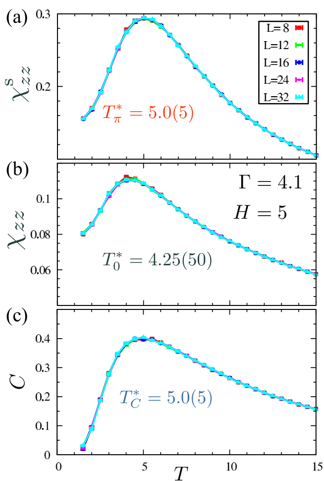
In the phase diagrams, we display the positions of broad peaks of $\chi_{zz}$ and $C$ in paramagnetic phase. It is well known that the magnetic susceptibilities exhibit a broad peak as a proximity effect near a finite-temperature tricritical point (e.g., [41]). Indeed, we confirm such a proximity effect in the case of finite-temperature tricritical point in Fig. 7(c): The both $T^{*}$s converge on the tricritical point, and the closer $H$ is to the tricritical point, the sharper the peaks are. The proximity effects for QTCP exists as well as those of the thermal tricritical point. We show an example of the proximity effect around the QTCP in Fig. 8. Only difference is that the broad peak of specific heat does not converge to the QTCP and stay at higher temperature. The reason is simply because the specific heat is zero at $T=0$, and does not diverge at the QTCP. In other words, the weaker the first-order quantum phase transition is, the weaker the proximity effect of specific heat is. In the case of the conventional QCP (Fig. 7(a)), $\chi_{zz}$ exhibits similar broad peak structure, and $T^{*}_{0}$ seems to converge into the QCP. However, $\chi_{zz}$ does not show divergence at the QCP and remains rather small value unlike the QTCP.

References

- [1] S. Sachdev, Quantum phase transitions (Wiley Online Library, 2007).
- [2] G. R. Stewart, Rev. Mod. Phys. 73, 797 (2001).
- [3] H. v. Löhneysen, A. Rosch, M. Vojta, and P. Wölfle, Rev. Mod. Phys. 79, 1015 (2007).
- [4] P. Gegenwart, Q. Si, and F. Steglich, Nat. Phys. 4, 186 (2008).
- [5] M. Suzuki, Progr. Theor. Phys. 56, 1454 (1976).
- [6] V. Zapf, M. Jaime, and C. D. Batista, Rev. Mod. Phys. 86, 563 (2014).
- [7] J. A. Hertz, Phys. Rev. B 14, 1165 (1976).
- [8] A. J. Millis, Phys. Rev. B 48, 7183 (1993).
- [9]
T. Moriya,
Spin fluctuations in itinerant electron
magnetism, vol. 56 (Springer-Verlag Berlin, 1985). - [10] T. Moriya and T. Takimoto, J. Phys. Soc. Jpn. 64, 960 (1995).
- [11] M. Imada, A. Fujimori, and Y. Tokura, Rev. Mod. Phys. 70, 1039 (1998).
- [12] T. Misawa and M. Imada, Phys. Rev. B 75, 115121 (2007).
- [13] I. M. Lifshitz, Sov. Phys. JETP 11, 1130 (1960).
- [14] Y. Yamaji, T. Misawa, and M. Imada, J. Phys. Soc. Jpn. 75, 094719 (2006).
- [15]
I. D. Lawrie and
S. Sarbach,
Phase Transition and Critical
Phenomena edited by C. Domb and J. L. Lebowitz, vol. 9 (Academic Press, London, 1984). - [16]
J. Cardy,
Scaling and renormalization in statistical
physics, vol. 5 (Cambridge university press, 1996). - [17] P. Gegenwart, J. Custers, Y. Tokiwa, C. Geibel, and F. Steglich, Phys. Rev. Lett. 94, 076402 (2005).
- [18] T. Misawa, Y. Yamaji, and M. Imada, J. Phys. Soc. Jpn. 77, 093712 (2008).
- [19] T. Misawa, Y. Yamaji, and M. Imada, J. Phys. Soc. Jpn. 78, 084707 (2009).
- [20] A. G. Green, S. A. Grigera, R. A. Borzi, A. P. Mackenzie, R. S. Perry, and B. D. Simons, Phys. Rev. Lett. 95, 086402 (2005a).
- [21] G. Giovannetti, C. Ortix, M. Marsman, M. Capone, J. van den Brink, and J. Lorenzana, Nat. Commun. 2, 398 (2011).
- [22] Y. Tokunaga, D. Aoki, H. Mayaffre, S. Krämer, M.-H. Julien, C. Berthier, M. Horvatić, H. Sakai, S. Kambe, and S. Araki, Phys. Rev. Lett. 114, 216401 (2015).
- [23]
H. Nishimori and
G. Ortiz,
Elements of Phase
Transitions and Critical Phenomena (Oxford University Press, 2010). - [24] T. Misawa, Y. Yamaji, and M. Imada, J. Phys. Soc. Jpn. 75, 064705 (2006).
- [25] J. Schmalian and M. Turlakov, Phys. Rev. Lett. 93, 036405 (2004).
- [26] A. G. Green, S. A. Grigera, R. A. Borzi, A. P. Mackenzie, R. S. Perry, and B. D. Simons, Phys. Rev. Lett. 95, 086402 (2005b).
- [27] P. Jakubczyk, J. Bauer, and W. Metzner, Phys. Rev. B 82, 045103 (2010).
- [28] K. Lukierska-Walasek, Acta. Phys. Pol. A 85, 381 (1994).
- [29] D. Carvalho and J. Plascak, Physica A 432, 240 (2015).
- [30] M. Mercaldo, I. Rabuffo, A. Naddeo, A. Caramico DAuria, and L. De Cesare, EPJ B 84, 371 (2011).
- [31] Y. Kato, D. Yamamoto, and I. Danshita, Phys. Rev. Lett. 112, 055301 (2014).
- [32] J. M. Kincaid and E. G. D. Cohen, Physics Reports 22, 57 (1975).
- [33] N. Kawashima and K. Harada, J. Phys. Soc. Jpn. 73, 1379 (2004).
- [34] H. G. Evertz, G. Lana, and M. Marcu, Phys. Rev. Lett. 70, 875 (1993).
- [35] Y. Kato and N. Kawashima, Phys. Rev. E 81, 011123 (2010).
- [36] U. Zülicke and A. J. Millis, Phys. Rev. B 51, 8996 (1995).
- [37] K. Harada, Phys. Rev. E 84, 056704 (2011).
- [38] A. Pelissetto and E. Vicari, Phys. Rep. 368, 549 (2002).
- [39] V. J. Emery, Phys. Rev. B 11, 3397 (1975).
- [40] D. Furman and M. Blume, Phys. Rev. B 10, 2068 (1974).
- [41] M. de Azevedo, C. Binek, J. Kushauer, W. Kleemann, and D. Bertrand, J. Magn. Magn. Mater. 140, 1557 (1995).
- [42] S. Nakatsuji, K. Kuga, Y. Machida, T. Tayama, T. Sakakibara, Y. Karaki, H. Ishimoto, S. Yonezawa, Y. Maeno, E. Pearson, et al., Nat. Phys. 4, 603 (2008).
- [43] Y. Matsumoto, S. Nakatsuji, K. Kuga, Y. Karaki, N. Horie, Y. Shimura, T. Sakakibara, A. H. Nevidomskyy, and P. Coleman, Science 331, 316 (2011).
- [44] K. Deguchi, S. Matsukawa, N. K. Sato, T. Hattori, K. Ishida, H. Takakura, and T. Ishimasa, Nat. Mater. 11, 1013 (2012).
- [45] S. Watanabe and K. Miyake, Phys. Rev. Lett. 105, 186403 (2010).
- [46] A. Ramires, P. Coleman, A. H. Nevidomskyy, and A. M. Tsvelik, Phys. Rev. Lett. 109, 176404 (2012).