Stochastic safety radius on Neighbor-Joining method and Balanced Minimal Evolution on small trees
Abstract
A distance-based method to reconstruct a phylogenetic tree with leaves takes a distance matrix, symmetric matrix with s in the diagonal, as its input and reconstructs a tree with leaves using tools in combinatorics. A safety radius is a radius from a tree metric (a distance matrix realizing a true tree) within which the input distance matrices must all lie in order to satisfy a precise combinatorial condition under which the distance-based method is guaranteed to return a correct tree. A stochastic safety radius is a safety radius under which the distance-based method is guaranteed to return a correct tree within a certain probability. In this paper we investigated stochastic safety radii for the neighbor-joining (NJ) method and balanced minimal evolution (BME) method for .
1 Introduction
A phylogenetic tree (or phylogeny) on the set is a graph which summarizes the relations of evolutionary descent between different species, organisms, or genes. Phylogenetic trees are useful tools for organizing many types of biological information, and for reasoning about events which may have occurred in the evolutionary history of an organism. There has been much research on phylogenetic tree reconstructions from alignments, and distance-based methods are some of the best-known phylogenetic tree reconstruction methods.
Once we compute pairwise distances from an alignment, we can reconstruct a phylogenetic tree via distance-based methods. In contrast with parsimony methods, distance-based methods have been shown to be statistically consistent in all settings (such as the long branch attraction) [7, 3, 4, 1]. Distance-based methods also have a huge speed advantage over parsimony and likelihood methods in terms of computational time, and hence enable the reconstruction of trees with large numbers of taxa. However, a distance-based method is not a perfect method to reconstruct a phylogenetic tree from the input sequence data set: in the process of computing a pairwise distance, we ignore interior nodes of a tree as well as a tree topology, and thus we lose information from the input sequence data sets. Therefore it is important to understand how a distance based method works and how robust it is with noisy data sets.
One way to measure its robustness is called the safety radius. A safety radius is a radius from a tree metric (a distance matrix realizing a true tree) within which the input distance matrices must all lie in order to satisfy a precise combinatorial condition under which the distance-based method is guaranteed to return a correct tree. More precisely, we have the following definition.
Definition 1.
Suppose we have a vector representation of all pairwise distances and suppose , where , is the set of all phylogenetic unrooted trees with leaves , and , where is the set of all non-negative real numbers, is a vector representation of the set of branch lengths in , is a tree metric, i.e., is the total of branch lengths in the unique path from a leaf to a leaf in . Let be the smallest interior branch length in . Then a method for reconstructing a phylogenetic -tree from each distance matrix on is said to have a safety radius if for any binary phylogenetic tree with leaves we have:
Notice that the definition of the safety radius defined in Definition 1 is deterministic even though the input data is a multivariate random variable. Thus, this is more meaningful to define in terms of probability distribution. Thus, in 2014 Steel and Gascuel introduced a notion of stochastic safety radius [9].
Definition 2 (Stochastic safety radius).
Suppose we allow to depend on : for some value . For any , we say that a distance-based tree reconstruction method has -stochastic safety radius if for every binary phylogenetic -tree on n leaves, with minimum interior edge length , and with the distance matrix on described by the random errors model, we have
In this paper we focus on two distance-based methods, namely neighbor-joining (NJ) method and balanced minimal evolution (BME) method. In 2002, Desper and Gascuel introduced a BME principle, based on a branch length estimation scheme of Pauplin [13]. The guiding principle of minimum evolution tree reconstruction methods is to return a tree whose total length (sum of branch lengths) is minimal, given an input dissimilarity map. The BME method is a special case of these distance-based methods wherein branch lengths are estimated by a weighted least-squares method (in terms of the input and the tree in question) that puts more emphasis on shorter distances than longer ones. Each labeled tree topology gives rise to a vector, called herein the BME vector, which is obtained from Pauplin’s formula. In 2000, Pauplin showed that the BME method is equivalent to optimizing a linear function, the dissimilarity map, over the BME representations of binary trees, given by the BME vectors [13]. Eickmeyer et. al. defined the BME polytope as the convex hull of the BME vectors for all binary trees on a fixed number of taxa. Hence the BME method is equivalent to optimizing a linear function, namely, the input distance matrix , over a BME polytope. They characterized the behavior of the BME phylogenetics on such data sets using the BME polytopes and the BME cones, i.e., the normal cones of the BME polytope.
The study of related geometric structures, the BME cones, further clarifies the nature of the link between phylogenetic tree reconstruction using the BME criterion and using the NJ Algorithm developed by Saitou and Nei [14]. In 2006, Gascuel and Steel showed that the NJ Algorithm, one of the most popular phylogenetic tree reconstruction algorithms, is a greedy algorithm for finding the BME tree associated to a distance matrix [8]. The NJ Algorithm relies on a particular criterion for iteratively selecting cherries; details on cherry-picking and the NJ Algorithm are recalled later in the paper. In 2008, based on the fact that the selection criterion for cherry-picking is linear in the distance matrix [2], Eickmeyer et. al. showed that the NJ Algorithm will pick cherries to merge in a particular order and output a particular tree topology if and only if the pairwise distances satisfy a system of linear inequalities, whose solution set forms a polyhedral cone in [5]. They defined such a cone as an NJ cone. In general, the sequence of cherries chosen by the NJ Algorithm is not unique, hence multiple distance matrix will be assigned by the NJ Algorithm to a single fixed tree topology The set of all distance matrix for which the NJ Algorithm returns a fixed tree topology is a union of NJ cones, however this union is not convex in general. Eickmeyer et. al. characterized those dissimilarity maps for which the NJ Algorithm returns the BME tree, by comparing the NJ cones with the BME cones, for eight or fewer taxa [5].
In this paper we use the BME cones and NJ cones in order to investigate their stochastic safety radius for . Here we assume that the multivariate random variable is defined as follows:
where , the Gaussian distribution with mean and a standard deviation , are independent for all pairwise distance . This paper is organized as follows: Section 2 shows the probability distribution of a random so that it satisfies the four point rule for all distinct quartets in with a fixed . Zarestkii in [11] defined the notion of the four point rule as follows: we select the tree topology (which means there is an internal edge between and for a distinct ) if
| (1) |
In Section 3 we will show multivariate probability distribution where is fixed and is the BME method, in Section 4 shows the multivariate probability distribution where is fixed and is the NJ method. Finally in Section 5 we will show some computational results on these probability distributions and we have shown the plot for the stochastic safety radii for the NJ and the BME methods varying and for (Figure 6). As shown in Figure 6 both stochastic safety radii are basically almost identical in this case since the probability distributions for the NJ and for the BME methods are almost identically same shown in Figure 5 for and .
2 Probability distribution on “four point rule”
For a tree containing random errors, the pairwise distance between two leaves is
where and are different taxas of a tree, is the true pairwise distance between taxa and , and follow i.i.d. Gaussian Distribution with mean 0 and variance . Intuitively in this section we are computing a probability distribution such that if we select a random , satisfies Equation 1 if and only if there is an internal edge between and in for all distinct . We find a formula for the probability, for 5 taxa, that a tree metric with random errors still obeys the original four-point inequalities on each subset of four leaves.

We first consider four point rule on 4 taxa tree. Suppose Figure 1 is the true tree. Then for a random tree, the following inequalities must be satisfied in order to return the correct tree:
| (2) |
Since
| (3) |
Then we can have
| (4) |
Since , we know . Let and be the density and cumulative distribution functions of , respectively. Then the probability that Inequality 4 is satisfied, i.e. the probability that a random distance matrix returns the true tree, equals to:
| (5) |
Now we consider four point rule on 5 taxa tree. Suppose the true tree is Figure 2(a). We need to check the rule on all possible combinations of four distinct leaves in this tree. It is trivial to see we only have 5 different combinations. For each of them, we could construct two inequalities similar to the way we obtained Equation 4. Therefore, we have 10 inequalities for the 5 combinations of 4 distinct taxa:
| (6) |
Let and
then the 10 inequalities are:
| (7) |
Thus the probability that a 5-leaved tree metric with random errors still obeys the original-four point inequalities on each subset of four leaves is the probability that inequality (7) is satisfied.
3 Probability distribution of the output tree via the BME method
This method begins with a given set of items and a symmetric (or upper triangular) square distance matrix whose entries are numerical dissimilarities, or distances, between pairs of items. From the distance matrix the BME method constructs a binary tree with the items labeling the leaves. The BME tree has the property that the distances between its leaves most closely match the given distances between corresponding pairs of taxa.
By “most closely match” in the previous paragraph we mean the following: the reciprocals of the distances between leaves are the components of a vector , and this vector minimizes the dot product where is the list of distances in the upper triangle of the distance matrix.
More precisely: Let the set of distinct species, or taxa, be called For convenience we will often let Let vector be given, having real valued components , one for each pair There is a vector for each binary tree on leaves also having components , one for each pair These components are ordered in the same way for both vectors, and we will use the lexicographic ordering: .
We define, following Pauplin [13]:
where is the number of internal nodes (degree 3 vertices) in the path from leaf to leaf The BME tree for the vector is the binary tree that minimizes for all binary trees on leaves Rather than the original fractional coordinates we will scale by a factor of giving coordinates
Since the furthest apart any two leaves may be is a distance of internal nodes, this scaling will result in integral coordinates. Thus we can equivalently say that the BME tree for the vector is the binary tree that minimizes for all binary trees on leaves
Consider a tree metric which arises from a binary tree with five leaves Let the interior edges and have lengths
Theorem 3.
Let , the tree for which is a tree metric, have cherries and
Let:
Let:
Then the BME method will return the correct tree if and only if:
Proof.
The BME method will return the correct tree if and only if
for all alternate trees This is true since the 1-skeleton of the BME polytope for is the complete graph on the 15 vertices.
Further, the above inequality holds iff
for all alternate trees Note that all the trees with five leaves have the same topology.
There are 14 other possible trees These separate into 5 sets of trees for which the left hand side of the above inequality is respectively or For each of these we collect the right hand sides, and take their maximum. ∎
4 Probability distribution of the output tree via the NJ method
4.1 H-representation of NJ cones [6]
Recall that the tree metric is a symmetric matrix with . We can flatten the entries in the upper triangle (diagonal entries are omitted) by columns:
where and . Let , , be the vector of tree metric after flattening. Notice here this flattening defines a one-to-one mapping between the indices:
In NJ algorithm, we first compute the Q-criterion (cherry picking criterion):
Similar as the flattened tree metric , the Q-criterion can also be flattened to a dimensional vector which can be obtained from by linear transformation:
where matrix is defined as:
where and .
Now each entry in corresponds to a pair of nodes in , the next step of NJ algorithm is to find the minimum entry of and join the corresponding two nodes as a cherry (“cherry picking”), then these two nodes will be replaced by a new node and the tree metric will be updated as (the dimension is reduced). We can see NJ algorithm proceeds by picking one cherry and reducing the size of the tree metric in each iteration until a binary tree is reconstructed. Without loss of generality and for the convenience of expression, we will only give details for the first iteration and assume the cherry we pick is in the rest part of this section.
First, to make cherry be the one to be picked, needs to be the minimum in . This means the following inequalities need to be satisfied:
Note that if an arbitrary cherry is picked, then a permutation of columns need to be assigned to .
Then, after picking cherry , we join these two nodes as the new node . Again, we can produce the new reduced tree metric from by linear transformation:
where ,
At last, after including inequalities in all iterations, by the shifting lemma in [6], we also include the following equalities: node ,
4.2 H-representation of 5 taxa NJ cones
There is only one tree topology for 5 taxa tree. Therefore, without loss of generality, we assume our true tree is Figure 2(a).


For 5 taxa tree, the flattening for tree metric is:
In Section 4.1, we can see that the permutation of columns for and depends on the cherry we pick. This means that we should compute NJ cones for all ordering of cherry picking (see the two orderings of cherry picking in Figure 2(b) for example).
There are four orderings of cherry picking. First we can pick cherry then pick cherry , which we denote as . Use a similar notation we have the other three: , , and . Take the ordering for example, use the results in Section 4.1 we can obtain the following linear constraints on :
Although it is not obvious to see, we found that the linear constraints for orderings and are exactly the same, and the linear constraints for orderings and are exactly the same. Therefore we only consider two NJ cones: the one for (denote as ), and the one for (denote as ).
4.3 Computing the probability that NJ reconstructs the correct 5 taxa tree
For the 5 taxa tree given in Figure 2(a) under the random errors model, we know that the flattened should follow a multi-variate normal (MVN) distribution with mean and covariance matrix . To trace the performance of NJ algorithm under different variation, we let to be a set of values in and then compute the probability that NJ algorithm reconstructs the correct tree for each value of .
For a given , it is trivial to see that the probability that NJ algorithm returns the right tree is .
We used software Polymake [10] and verified that the dimension of is lower than both of them, therefore . Polymake also gives us the facets of these two NJ cones. For example, the facets of are:
With these facets, we can use the R function “pmvnorm{mvtnorm}” with GenzBretz algorithm to compute and .
5 Computational experiments
In this section, we show both the theoretical and simulation probabilities that the four point rule reconstructs the correct tree, as well as NJ algorithm and BME method. In our computational experiments, we set all branch lengths to be ’s and compute the probabilities for different values of .

In Figure 3, when is increasing, the probability of 5 taxa tree will dramatically decrease faster than the probability of 4 taxa tree because we have more constraints to satisfy in 5 taxa tree which leads to lower probabilities.
In Figure 4(a), we calculated the theoretical probability that the NJ method reconstructs the correct 5 taxa tree based on Section 4. For the simulation, we fix the 5 taxa tree in Figure 2(a) with all branch lengths to be , and add i.i.d. normal random errors to the pairwise distance matrix. Then we use R function “nj{ape}” from the “ape” package in R [12] to reconstruct the tree. If the RF distance equals 0, it means that NJ method successfully returns the correct tree. Our simulation is based on 10,000 random trees. Figure 4(a) shows that the theoretical probabilities perfectly match the simulation result.

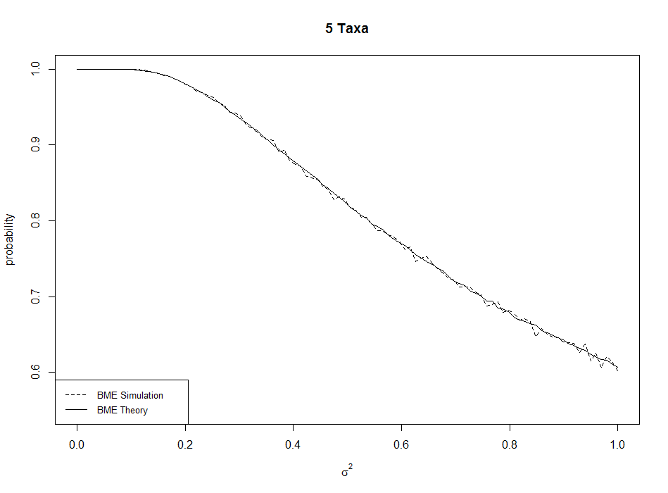


In Figure 4(b), we calculated the theoretical and simulated probabilities that the BME method will return the correct 5 taxa tree. For the theoretical probability, we generate 100,000 sets of random errors, and check whether the theoretical rule is satisfied. In the end, we return the percentage. For the simulation, we generate random trees in the similar way to what we did for NJ algorithm. Then we used R function “fastme.bal{ape}” to reconstruct the tree. Again we used RF distance to check if the BME method successfully returned the correct tree. Our simulation is based on 10,000 random trees. Figure 4(b) shows that the theoretical probabilities perfectly match the simulation result.
Figure 5 shows that there is almost no difference between BME and NJ methods on 5 taxa tree in both theoretical probabilities and simulation result.
Acknowledgements
Stefan Forcey would like to thank the American Mathematical Society and the Mathematical Sciences Program of the National Security Agency for supporting this research through grant H98230-14-0121.11 1 This manuscript is submitted for publication with the understanding that the United States Government is authorized to reproduce and distribute reprints.
References
- [1] M. Bordewich, O. Gascuel, K. T. Huber, and V. Moulton. Consistency of topological moves based on the balanced minimum evolution principle of phylogenetic inference. IEEE/ACM Trans. Comput. Biology Bioinform., 6(1):110–117, 2009.
- [2] D Bryant. On the uniqueness of the selection criterion in neighbor-joining. J. Classif., 22:3–15, 2005.
- [3] Ronald W. DeBry. The consistency of several phylogeny-inference methods under varying evolutionary rates. Mol Biol Evol, 9(3):537–551, 1992.
- [4] F. Denis and O. Gascuel. On the consistency of the minimum evolution principle of phylogenetic inference. Discrete Applied Mathematics, 127(1):63–77, 2003.
- [5] K. Eickmeyer, P. Huggins, L. Pachter, and R. Yoshida. On the optimality of the neighbor-joining algorithm. Algorithms for Molecular Biology, 3(5), 2008.
- [6] Kord Eickmeyer and Ruriko Yoshida. R: Geometry of neighbor-joining algorithm for small trees. In Proceedings of the third international conference on Algebraic Biology, 2008.
- [7] J. Felsenstein. Cases in which parsimony or compatibility methods will be positively misleading. Syst. Zool., 22:240–249, 1978.
- [8] O Gascuel and M Steel. Neighbor-joining revealed. Molecular Biology and Evolution, 23(11):1997–2000, 2006.
- [9] O. Gasquel and M. Steel. A ’stochastic safety radius’ for distance-based tree reconstruction, 2014.
- [10] E Gawrilow and M Joswig. polymake: an approach to modular software design in computational geometry. In Proceedings of the 17th Annual Symposium on Computational Geometry, pages 222–231. ACM, 2001. June 3-5, 2001, Medford, MA.
- [11] Zarestkii K. Reconstructing a tree from the distances between its leaves (in russian). Uspehi Mathematicheskikh Nauk, 20:90–92, 1965.
- [12] E. Paradis, J. Claude, and K. Strimmer. APE: analyses of phylogenetics and evolution in R language. Bioinformatics, 20:289–290, 2004.
- [13] Y. Pauplin. Direct calculation of a tree length using a distance matrix. J. Mol. Evol., 51:41–47, 2000.
- [14] N Saitou and M Nei. The neighbor joining method: a new method for reconstructing phylogenetic trees. Molecular Biology and Evolution, 4(4):406–425, 1987.