Monte Carlo study of the frame, fluctuation and internal tensions of fluctuating membranes with fixed area

Let us consider an incompressible, fluctuating lipid membrane with a fixed area $A=A_{0}$, corresponding to a fixed number of lipids. We assume that it is attached to a deformable frame, of variable area $A_{\rm p}$, that exerts onto the membrane a fixed tension $\tau$. The Hamiltonian of the system is thus given by[1]

where $H=c_{1}+c_{2}$ represents the sum of the two principal curvatures of the membrane. The Gaussian bending modulus[1] $\bar{\kappa}$ has been neglected, according to the Gauss–Bonnet theorem, which is correct for fixed angular boundary conditions or periodic boundary conditions along the frame[32].

We use the Monge representation, in which the membrane shape is describe by its height $z=h(x,y)$ above the plane of the frame. Note that this parametrisation does not require the membrane deformation to be small. The only restriction is that overhangs are forbidden, since the function $h$ is single valued. In this representation, the total curvature $H$ is exactly given by[33]

where subscripts represent spatial derivatives, e.g., $h_{x}=\partial h/\partial x$. We work here in the non-linear regime, allowing for large deformations of the membrane, i.e., we do not use the custom linear approximation $H\simeq h_{xx}+h_{yy}$ (employed in the Gaussian framework). Note that in our simulations (see the details below) the maximum slope, $\mathrm{max}(|h_{x}|)$, reaches 1.3 at vanishing frame tension, but does not exceed this value. This justifies both using the exact expression for $H$ and neglecting overhangs. Close to the buckling transition, however, i.e., for large negative frame tensions, these assumptions may not be valid.

Because it is quite difficult to work with a fixed area $A=A_{0}$, we change ensemble in order to control the conjugated internal tension $\sigma$, instead of the membrane area $A$. In the thermodynamic limit, the two ensembles are expected to be equivalent. Indeed, as shown in Appendix A, we find quantitatively similar results in the ensemble in which the real area $A$ is almost prescribed by means of a quadratic potential. In this stress–controlled ensemble, the modified Hamiltonian weighting the membrane fluctuations is given by

with $\langle A\rangle=A_{0}$ systematically enforced by adjusting $\sigma$.

In order to implement the membrane fluctuations numerically, we introduce a $N_{x}\times N_{y}$ lattice on the plane $(x,y)$ of the frame, with lattice spacing $a$. The height of the membrane surface is defined by $h_{ij}$ on each lattice site, with $1\leq i\leq N_{x}$ and $1\leq j\leq N_{y}$. In the reminder of this paper, we take $N_{x}=N_{y}=\sqrt{N}$. Furthermore, we adopt periodic boundary condition. Thus the projected area is given by $A_{\rm p}=Na^{2}$.

Importantly, because the number of lipids is fixed while the frame area $A_{\rm p}$ is variable, we take $N$ constant but $a$ variable. In other words, in our simulation the lattice spacing is not fixed. We stress, however, that $a$ always remains uniform over the lattice: it is the overall lattice spacing that changes. Therefore the projection over the reference plane of the vertices always maps onto a square grid of finite spacing and the vertices can never overlap. Note that a similar lattice membrane model (with fixed spacing and the Gaussian approximation) has been employed for Monte Carlo simulation in order to investigate inclusions effects [34].

Monte Carlo simulations are performed with the lattice heights $\{h_{ij}\}$ and the lattice spacing $a$ as dynamical variables. Special care is required, however, for the sampling of the height variables. In the Monge gauge, each site can only fluctuate in the $z$ direction, whereas in the physical gauge, because the membrane is fluid, the relevant fluctuations occur by local displacements along the membrane’s normal. In order to avoid an artificial entropy increase of the states where the membrane is tilted, the naive measure $d^{N}[h]=\prod_{i,j}dh_{ij}/\delta_{0}$, where $\delta_{0}$ is a quantum of height fluctuations, must be transformed to

Here, $\theta_{ij}$ is the angle between the normal vector of the site $(i,j)$ and the $z$ axis, and $\cos\theta_{ij}=1/\sqrt{1+h_{x}^{2}+h_{y}^{2}}$. In this way, the quantum height displacement in the normal direction is always $\delta_{0}$. Equivalently, we can keep the naive measure $d^{N}[h]$ and add to the Hamiltonian the following correction term:

where $T$ is the temperature and $k_{\mathrm{B}}$ Boltzmann’s constant. Note that this correction, that would be exact if the membrane was uniformly tilted, is only approximate if the tilt changes from site to site. In practice, it works well when the membrane slope is small, as in the present simulations. For highly tilted membranes, such as buckled membranes, the correction term, eqn (5), is not sufficient, as discussed in Appendix B.

The partition function in the stress–controlled ensemble introduced above is given by

with $\mathcal{H}^{\prime}=\mathcal{H^{\star}}+\mathcal{H}_{\rm{corr}}$. Metropolis sampling is employed [35]. In each Monte Carlo step, $N$ trial moves of the height of a random site are attempted. The change of $a$ (hence $A_{\rm p}$) is attempted every $5$ Monte Carlo steps. The amplitudes of the $h_{ij}$ and $A_{\rm p}$ changes are adjusted so that the rejection rate lies in the range 40%–60%. Both $A$ and $A_{\rm p}$ change during the simulations. However, for a given Monte Carlo run at a specified value of $\tau$, the internal tension $\sigma$ is adjusted in order for the average of the membrane area $\langle A\rangle$ to have the specific value $A_{0}$, fixed once for all.

In our simulation, the real area $A$ of the membrane is calculated as follows. The local area associated to a site $P(i,j)$ is obtained as one half of the total area of the four triangles [APB], [BPC], [CPD] and [DPA] built from the neighbouring sites of coordinates:

The area of each triangle can be calculated by using height differences between the lattice sites. Then, the total real area can be expressed as

Simulation are carried out at least for $10^{7}$ steps after the initial relaxation. The statistical errors are calculated from four or more independent runs.

Since our simulated membrane has a prescribed average area $A_{0}$ and a fixed number $N$ of degrees of freedom, we can picture each degree of freedom as a patch of lipids of fixed average area $a_{0}^{2}=A_{0}/N$. In the following we are going to nondimensionalise the lengths by $a_{0}$ (the size of a degree of freedom in the membrane) and the energies by $k_{\mathrm{B}}T=4\times 10^{-21}$ J (room temperature energy). In other words, we shall set $a_{0}=k_{\mathrm{B}}T=1$. Hence, all tensions will be given in units of $k_{\mathrm{B}}T/a_{0}^{2}$. As previously discussed, we shall thus adjust $\sigma$ for each $\tau$ in order to have systematically $\langle A\rangle=N$, in dimensionless units.

Let us estimate tension scale $k_{\mathrm{B}}T/a_{0}^{2}$. In principle, we are free to choose the linear size $a_{0}$ of the lipid patches that constitute our degrees of freedom. It is convenient, however, to choose the smallest possible size, in order to allow for all possible fluctuations and to avoid using renormalised elastic constants. Owing to the level of coarse-graining of our simulation, in which the bilayer membrane of real thickness $\approx\!5$ nm is treated as a mathematical surface, it is natural to think of the lipid patches as regions of typical size, e.g. $a_{0}\approx 20~\text{nm}$. Then, the natural unit of tension in our simulation is $k_{\mathrm{B}}T/a_{0}^{2}\approx 10^{-5}$ J/m². The tension mechanically imposed on ordinary vesicle membranes, in experiments, are in the range $10^{-7}$ J/m²–$10^{-2}$ J/m², where the smallest value corresponds to floppy vesicles and the largest value corresponds to the lytic tension[36]. We shall therefore have $\tau$ span the range $10^{-2}$–$10^{3}$ in dimensionless units. Let us stress that this corresponds to five orders of magnitude.

In our simulation, we choose a specific value of the bending rigidity corresponding to $\kappa=10~k_{\mathrm{B}}T$, i.e., $\kappa=10$ in dimensionless units. We shall consider membrane sizes corresponding to $N=400,1600,6400$ and $25600$. With the value of $a_{0}$ given above, this corresponds to membrane of linear dimension $\sqrt{A_{0}}=\sqrt{N}a_{0}=400$ nm, $800$ nm, $1.6~\mu$m and $3.2~\mu$m, respectively. These values are quite small if one thinks of macroscopic experiments, but they are reasonably large on the biological scale. Because of the change of ensemble that we have performed, we shall check the convergence of our results with increasing $N$.

In Fig. 1, a simulation snapshot for $N=6400$ is shown in the tensionless state $\tau=0$.

From now, unless otherwise specified, all quantities will be given in dimensionless units (see Sec. II.3). We investigate here the relationship between $\sigma$ and $\tau$. As explained above, we place ourselves in the $(\sigma,\tau)$ ensemble; however, for every imposed frame tension $\tau$, we determine the internal tension $\sigma$ that achieves $\langle A\rangle=N$. Our simulated membrane thus effectively has a constant real area (up to fluctuations that become irrelevant in the thermodynamic limit). Simulations in the $(A,\tau)$ ensemble, where $A$ is nearly fixed by means of a steep quadratic potential, are discussed in Appendix A.

The determined values of $\sigma$ are plotted in Fig. 2a against the frame tension for different system sizes: $N=400,1600,6400$ and $25600$. For any value of $\tau$ we find $\sigma>\tau$. Data for both positive and negative frame tensions are displayed together as a function of $|\tau|$: the upper branch corresponds to $\tau>0$ and the lower branch corresponds to $\tau<0$. Note that for $\tau>0$ the difference between $\sigma$ and $\tau$ is sizeable only for small values of the frame tension. For $\tau=0$ we find that the residual internal tension is equal to $\sigma_{0}\simeq 0.500\pm 0.001$, where the error bar takes into account the determinations using different values of $N$. In other words, the residual tension turns out to be fairly independent of system size.

When $\tau$ decreases below some negative threshold $\tau_{b}<0$, the membrane buckles either into the $x$ or the $y$ direction: the average membrane shape undergoes a transition from flat to non-flat through a symmetry breaking (like a rod under compression). Note that the membrane height function remains single valued although it acquires a bimodal distribution. The absolute value $|\tau_{b}|$ of the buckling threshold decreases as the system size $N$ gets larger. In the lower branch, the data points for $|\tau|>|\tau_{b}|$, in the buckling state, are eliminated from the plots in Figs. 2a and 3. It is notable that the condition $\sigma<0$ is not required for the buckling transition. We also simulated our lattice model in the $(A_{\rm p},\sigma)$ ensemble, i.e. with constant lattice spacing $a$ and freely changing membrane area $A$. We found that the membrane buckles then at $\sigma=0$. These results suggest that $\sigma$ is not the mechanical force that drives membrane buckling.

In Ref.20, the difference between the tensions $\sigma$ and $\tau$ was calculated within the Gaussian approximation, yielding

where $\Lambda$ is the ultraviolet wavevector cutoff and all quantities have their normal dimensions. Within our simulation, this ultraviolet cutoff corresponds to the lattice spacing. We thus expect

Whereas our simulation is fully nonlinear, the expression for $\sigma-\tau$ calculated within the Gaussian approximation fits the data quite well (Fig. 2b). Since the numerical value of $\langle a\rangle$ changes by only $1.4$% from $\tau=0$ to $1000$, we use for the fit the extreme value at high tension, $a=1$. The best fit of the data gives then $\alpha=1.12$, very close to unity.

Thermodynamic limit.—In Fig. 3, we plot the two tensions $\sigma$ and $\tau$ against the excess area $(A-A_{\rm p})/A$ for the various system sizes $N=400,1600,6400$ and $25600$. Here, only positive values of $\tau$ are displayed: the downwards divergence of the curves associated to the plain circles corresponds to $\tau\to 0$. The system size dependence is marked for small sizes, but the data appears to converge to a universal thermodynamic limit at large system sizes. Finite size effects are more or less irrelevant for $N\geq 6400$.

We now discuss the fluctuation tension $r$. It is derived from the spectrum density, assumed to take the standard form[33]:

where $h(\bm{q})$ is the Fourier transform of the height function, with $\bm{q}$ the wavevector. The fluctuation tension $r$ and the bending rigidity $\kappa_{r}$, appearing in the fluctuation spectrum, are the renormalised counterparts of the Hamiltonian parameters $\sigma$ and $\kappa$.

In estimating these quantities using simulation results, it is crucially important to consider large-scale fluctuations. However, because we always treat finite-size systems, the wavevector spectrum is limited, which results in systematic deviations. Previously, two of the present authors have been addressed in detail the question of the estimation for the bending rigidity from simulation data[8]. For a planar membrane, the correct value of the bending rigidity can be determined uniquely by first estimating the rigidity $\kappa_{r}$ via a fit of the inverse spectrum $(rq^{2}+\kappa_{r}q^{4})/(k_{\mathrm{B}}T)$ in the wavevector range $2\pi/(a_{0}\sqrt{N})\leq q<q_{\mathrm{cut}}$, then by extrapolating the results to the limit $q_{\rm cut}\to 0$, where $q_{\mathrm{cut}}$ is a varying upper fitting wavevector limit. Note that because the projected area $A_{\rm p}$ fluctuates, there is some ambiguity regarding the definition of the quantified wavevectors. As discussed in Appendix C, our results are not sensitive to those details. This procedure has been carried out for the present system. We find that the value of $\kappa_{r}$ coincides with the bare value $\kappa$, up to our numerical precision. This result makes sense because renormalisation group calculations predict

up to a numerical factor of order unity[33] (here all quantities have their normal dimensions). This prediction gives $\Delta\kappa/\kappa\approx 0.03$ for $N=6400$, which is less than the error bars, and thus not detectable in our simulation.

The correct value of the fluctuation tension $r$ (the renormalised tension) can be estimated likewise in the limit $q_{\rm cut}\to 0$. For finite values of $q_{\rm cut}$, we find that $r$ is overestimated but converges in the limit $q_{\rm cut}\to 0$ to a well defined value. The corresponding extrapolation is performed by using a quadratic function of $q_{\rm cut}$. The fitting was performed in the range $0.015\leq(q_{\rm cut}/\pi)^{2}<0.15$.

Figure 4 shows the values of the fluctuation tension $r$. We find that $r$ is fairly close to $\tau$ for all the investigated values of $\tau$, as indicated in Fig. 4a. In Fig. 4b, the difference $r-\tau$ is plotted against $\tau$. For large system sizes, $N=6400$ and $25600$, we observe a small deviation between $r$ and $\tau$; however, as discussed in Appendix B, we believe that this deviation is smaller than a possible systematic error arising from the measure correction.

In the present work, all the nonlinearities of the problem have been taken into account: (i) the nonlinear expression of the membrane elementary area $dA$ (ii) the nonlinear expression of the membrane bending energy density $H^{2}dA$, and (iii) the nonlinear measure correction $\mathcal{H}_{\text{corr}}$ dealing with the excess entropy of the Monge gauge. The Gaussian approximation, which is frequently used in basic calculations, consists in replacing the bending energy density $H^{2}dA$ by $H_{\rm L}^{2}dA_{\rm p}$, where $H_{\rm L}=h_{xx}+h_{yy}$ is the Laplacian approximation of the mean-curvature and $dA_{p}$ the projected elementary area, and in neglecting the entropy measure correction $\mathcal{H}_{\text{corr}}$. Indeed, at quadratic order, the measure correction becomes $\frac{1}{2}k_{\mathrm{B}}T\sum_{i,j}\theta_{ij}^{2}\simeq\frac{1}{2}k_{\mathrm{B}}T\sum_{i,j}(\nabla h)^{2}_{ij}$, which is of no consequences as it simply redefines the tunable parameter $\sigma$. In this subsection, we investigate how these two Gaussian approximations affect the surface tensions. First, we make the Laplacian approximation, i.e., $H^{2}dA$ is replaced by $H_{\rm L}^{2}dA_{\rm p}$ in eqn (1), and we keep the entropy correction term $\mathcal{H}_{\text{corr}}$. The corresponding results are denoted by the subscript EL in Fig. 5. Then we also remove the entropy correction term. The corresponding calculations are denoted by the subscript L.

We find that the internal tension $\sigma$ is not changed by these modifications. However, $r_{\rm EL}$ and $r_{\rm L}$ are significantly different from $r$, as shown in Fig. 5. Using the Laplacian approximation while keeping the entropy correction term results in a fluctuation tension $r_{\rm EL}$ about three times larger than $\sigma$. Further removing the entropy correction yields a tension $r_{\rm L}$ very close to $\sigma$, in agreement with the well-known coincidence of $r$ and $\sigma$ at the Gaussian level. Therefore, the effects of the measure correction and of the nonlinear curvature are opposite to each other: the former raises the value of $r$, the latter lowers it. Both of these effects need to be taken into account for a faithful description of the membrane fluctuations beyond the level of the Gaussian approximation, and the estimated $r$ deviates from the true value if either of them is missing. Note that without the entropy correction term, $\mathcal{H}_{\rm corr}$, the nonlinear bending energy leads to an enhancement of the vertical motion of the sites, resulting in the collapse of the simulations.

In the body of this paper, the real area $A$ of the membrane is not fixed, but its average value $\langle A\rangle$ is controlled by the parameter $\sigma$ (much as the average number of particles in a grand-canonical ensemble is controlled by the chemical potential). In principle, we have checked the validity our results by studying the thermodynamic limit of increasing system sizes. It is nonetheless interesting to test our results by working in the ensemble in which the area $A$ is prescribed. This is the purpose of the present Appendix.

While it is very difficult to prescribe exactly the membrane area, because it is difficult to identify the sampling condition that satisfy this constraint, one can easily almost prescribe the area by using a quadratic potential of tunable strength $K_{\mathrm{A}}$. We thus worked with the Hamiltonian

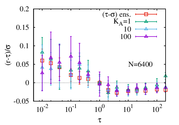
We have performed the corresponding Monte-Carlo simulations exactly in the same manner as in the body of the paper. Figure 6 shows the result of these additional simulations, for $K_{\mathrm{A}}=1$, 10 and 100, with $N=6400$, and compares them with the results of Fig. 4. With increasing $K_{\mathrm{A}}$, the standard deviation of the real area decreases: 0.01%, 0.001%, and 0.0003%, for $K_{\mathrm{A}}=1,\ 10,$ and $100$, respectively. With larger values of $K_{\mathrm{A}}$, the fluctuations of the membrane area become suppressed so that unbiased equilibrium sampling is impossible.

To check the reliability of the measure correction $\mathcal{H}_{\text{corr}}$, eqn (5), we performed simulations in which the entire membrane is tilted by an angle $\theta_{\rm a}$. The periodic boundary condition along the $x$ direction is modified to $h(N_{x},j)=h(0,j)+N_{x}a\sin\theta_{\rm a}$. The $x$ side length of the lattice is changed to $a\cos\theta_{\rm a}$ in order to maintain a square grid in the tilted projected plane. The height spectrum is calculated for the tilted plane, of normal vector $(-\sin\theta_{\rm a},0,\cos\theta_{\rm a})$. The fluctuation tension $r$ increases with increasing $\theta_{\rm a}$ (see Fig. 7), while $\sigma$ is independent of $\theta_{\rm a}$. This implies that the excess entropy associated with the membrane tilt in the Monge gauge is not completely removed. However, the deviation is small for small $\theta_{\rm a}$, and the overestimation of $r$ is less than 0.1 for $\theta_{\rm a}<0.1\pi$. In our simulation, at $\tau=0$ we obtain $\langle\cos\theta_{ij}\rangle=0.98$, i.e., the mean angle is $0.066\pi$. We conclude that the obtained values of $r$ are reliable within the accuracy of $0.1$ (in dimensionless units).

In Sec. III.2, the renormalised tension $r$ is calculated by fitting the height spectrum $\langle|h(\bm{q})|^{2}\rangle$. We use a sequence of instantaneous height configurations, and we perform averages after the simulation finishes. Because the projected area $A_{\rm p}$ changes during the simulations, the wavevectors on the reciprocal lattice are not fixed. They are given by

where $n$ and $m$ are integers. All these data are mapped to a one-dimensional wavevector $q=|\bm{q}|$. In plotting $\langle|h(q)|^{2}\rangle$, the data of $|h(\bm{q})|^{2}$ are averaged over close values of $q$ (the width of $q$ bins is $b\pi/\sqrt{N}$. Here, $b=1.2$ is taken) and over all the height configurations.

We have confirmed the robustness of our estimation of $r$, by using a different set of wavevectors, defined by

For each of integers $n,m$, the values of $\langle|h(\bm{q}^{\prime})|^{2}\rangle$ is averaged over the sequence of instantaneous height configurations. The results obtained by these two methods do not essentially differ from one another: the differences in the value of $r$ are smaller than $0.025~k_{\mathrm{B}}T/a_{0}^{2}$ for all $\tau$, which is typically smaller than the error bars.

References

- [1] W. Helfrich, Z. Naturforsch., 1973, 28c, 693–703.
- [2] R. Goetz, G. Gompper and R. Lipowsky, Phys. Rev. Lett., 1999, 82, 221–224.
- [3] E. Lindahl and O. Edholm, Biophys. J., 2000, 79, 426–433.
- [4] W. K. Den Otter and W. J. Briels, J. Chem. Phys., 2003, 118, 4712–4720.
- [5] O. Farago and P. Pincus, J. Chem. Phys., 2004, 120, 2934–2950.
- [6] V. A. Harmandaris and M. Deserno, J. Chem. Phys., 2006, 125, 204905.
- [7] H. Noguchi and G. Gompper, Phys. Rev. E, 2006, 73, 021903.
- [8] H. Shiba and H. Noguchi, Phys. Rev. E, 2011, 84, 031926.
- [9] H. Noguchi, Phys. Rev. E, 2011, 83, 061919.
- [10] M. Hu, P. Diggins IV and M. Deserno, J. Chem. Phys., 2013, 138, 214110.
- [11] P. Tarazona, E. Chacón and F. Bresme, J. Chem. Phys., 2013, 139, 094902.
- [12] M. C. Watson, A. Morriss-Andrews, P. M. Welch and F. L. H. Brown, J. Chem. Phys., 2013, 139, 084706.
- [13] M. Hu, J. J. Briguglio and M. Deserno, Biophys. J., 2012, 102, 1403–1410.
- [14] A. Imparato, J. Chem. Phys., 2006, 124, 154714.
- [15] O. Farago, Phys. Rev. E, 2011, 84, 051914.
- [16] J. B. Fournier, A. Ajdari and L. Peliti, Phys. Rev. Lett., 2001, 86, 4970–4973.
- [17] F. David and S. Leibler, J. Phys. II, 1991, 1, 959–976.
- [18] K. Sengupta and L. Limozin, Phys. Rev. Lett., 2010, 104, 088101.
- [19] O. Farago and P. Pincus, Eur. Phys. J. E, 2003, 11, 399–408.
- [20] J.-B. Fournier and C. Barbetta, Phys. Rev. Lett., 2008, 100, 078103.
- [21] F. Schmid, EPL, 2011, 95, 28008; Comment: J.-B. Fournier, EPL, 2012, 97, 18001; Reply: F. Schmid, EPL, 2012, 97, 18002.
- [22] W. Cai, T. C. Lubensky, P. Nelson and T. Powers, J. Phys. II, 1994, 4, 931–949.
- [23] H. Diamant, Phys. Rev. E, 2011, 84, 061123.
- [24] S. J. Marrink and A. E. Mark, J. Phys. Chem. B, 2001, 105, 6122–6127.
- [25] Z. J. Wang and D. Frenkel, J. Chem. Phys., 2005, 122, 234711.
- [26] G. Brannigan and F. L. H. Brown, Biophys. J., 2006, 90, 1501–1520.
- [27] B. West, F. L. H. Brown and F. Schmid, Biophys. J., 2009, 96, 101–115.
- [28] J. Neder, B. West, P. Nielaba and F. Schmid, J. Chem. Phys., 2010, 132, 115101.
- [29] J. Stecki, J. Chem. Phys., 2006, 125, 154902.
- [30] Y. Y. Avital and O. Farago, J. Chem. Phys., 2015, 142, 124902.
- [31] E. Evans and W. Rawicz, Phys. Rev. Lett., 1990, 64, 2094–2097.
- [32] B S. Buchin, Lectures on Differential Geometry, World Scientific, Singapore, 1980.
- [33] S. A. Safran, Statistical thermodynamics sof surfaces, interfaces, and membranes, Addison-Wesley, Massachusetts, 1994.
- [34] T. R. Weikl, Europhys. Lett., 2001, 54, 547–553.
- [35] D. P. Landau and K. Binder, A Guide to Monte-Carlo Simulations in Statistical Physics, Cambridge University Press, Cambridge, 3rd edn., 2009.
- [36] W. Rawicz, K. C. Olbrich, T. McIntosh, D. Needham and E. Evans, Biophys. J., 2000, 79, 328–339.