跳到论文正文
W Papers独立论文阅读器 arXiv:1507.08566 论文正文 计算阅读时间 · 0%
引用这篇论文根据当前论文元数据生成,正式投稿前建议核对。


License: arXiv.org perpetual non-exclusive license
arXiv:1507.08566v4 [cs.DC] 01 Oct 2015

Diffusion Adaptation Over Clustered Multitask Networks Based on the Affine Projection Algorithm

Vinay Chakravarthi Gogineni, Mrityunjoy ChakrabortyDepartment of Electronics and Electrical Communication EngineeringIndian Institute of Technology, Kharagpur, INDIAPhone: +91−3222−283512+91-3222-283512\quad Fax: +91−3222−255303+91-3222-255303    E.Mail :  vinaychakravarthi@ece.iitkgp.ernet.in    mrityun@ece.iitkgp.ernet.in
Abstract

Distributed adaptive networks achieve better estimation performance by exploiting temporal and as well spatial diversity while consuming few resources. Recent works have studied the single task distributed estimation problem, in which the nodes estimate a single optimum parameter vector collaboratively. However, there are many important applications where the multiple vectors have to estimated simultaneously, in a collaborative manner. This paper presents multi-task diffusion strategies based on the Affine Projection Algorithm (APA), usage of APA makes the algorithm robust against the correlated input. The performance analysis of the proposed multi-task diffusion APA algorithm is studied in mean and mean square sense. And also a modified multi-task diffusion strategy is proposed that improves the performance in terms of convergence rate and steady state EMSE as well. Simulations are conducted to verify the analytical results.

I Introduction

Distributed adaptation over networks has emerged as an attractive and challenging research area with the advent of multi-agent( wireless or wireline) networks. Recent results in the field can be found in [1]-[3]. In adaptive networks, the interconnected nodes continuously learn and adapt, as well as perform the assigned tasks such as parameter estimation from observations collected by the dispersed agents. Consider a connected network consisting of NN nodes observing temporal data arising from different spatial sources with possibly different statistical profiles. The objective is to enable the nodes to estimate a parameter vector of interest, wo​p​tw_{opt} from the observed data. In a centralized approach, the data or local estimates from all nodes would be conveyed to a central processor where they would be fused and the vector of parameters estimated. In order to reduce the requirement of powerful central processor and extensive amount of communications in a traditional centralized solution, a distributed solution is developed relying only on local data exchange and interactions between intermediate neighborhood nodes, while retaining the estimation accuracy of centralized solution. In distributed networks, the individual nodes share the computational burden so that communications are reduced as compared to the centralized network, and power and bandwidth usage are also there by reduced. Due to these merits, distributed estimation has received more attention recently and been widely used in many applications, such as in precision agriculture, environmental monitoring, military surveillance, transportation and instrumentation.

The mode of cooperation that is allowed among the nodes determines the efficiency of any distributed implementation. In incremental mode of cooperation, each node transfers information to its corresponding adjacent node in sequential manner using cyclic pattern of collaboration. This approach reduces communications between nodes and improves the network autonomy as compared the centralized solution. In practical wireless sensor networks, it may be more difficult to establish a cyclic pattern as required in the incremental mode of cooperation as the number of sensor nodes increase. On the other hand, in diffusion mode of cooperation, each node exchanges information with its neighborhood (i.e., the set of all its neighbors including itself), 𝒩k\mathcal{N}_{k} as directed by the network topology. There exist several useful distributed strategies for sequential data processing over networks including consensus strategies [4]-[6], incremental strategies [7]-[9] and diffusion strategies [10]-[13]. Diffusion strategies exhibit superior stability and performance over consensus based algorithms [14].

The existing literature on distributed algorithms shows that most works focus primarily on the case where the nodes estimate a single optimum parameter vector collaboratively. We shall refer to problems of this type as single-task problems. However, many problems of interest happen to be multi-task oriented i.e., consider the general situation where there are connected clusters of nodes, and each cluster has a parameter vector to estimate. The estimation still needs to be performed cooperatively across the network because the data across the clusters may be correlated and, therefore, cooperation across clusters can be beneficial. This concept is relevant to the context of distributed estimation and adaptation over networks. Initial investigations along these lines for the traditional diffusion strategy appear in [15]-[19]. It is well known that in the case of a single adaptive filter, one major drawback of the LMS algorithm is its slow convergence rate for colored input signals and the APA algorithm is a better alternative to LMS is such an environment. For distributed networks, highly correlated inputs also deteriorate the performance of the multi-task diffusion-LMS (multi-task d-LMS) algorithm. In this paper we therefore focus on a new APA-based multi-task distributed learning scheme over networks to obtain a good compromise between convergence performance and computational cost and to analyze their performance in terms of mean-square error and convergence rate.

II Network Models and Multi Task learning

Consider a network with NN nodes deployed over a certain geographical area. At every time instant nn, every node kk has access to time realizations {dk​(n),uk​(n)}\{d_{k}(n),\textbf{u}_{k}(n)\} with dk​(n)d_{k}(n) denoting a scalar zero mean reference signal and uk​(n)\textbf{u}_{k}(n) is an L×1L\times 1 regression vector, uk​(n)=[uk​(n),uk​(n−1),…,uk​(n−L+1)]T\textbf{u}_{k}(n)=[u_{k}(n),u_{k}(n-1),...,u_{k}(n-L+1)]^{T} with covariance matrix Ru,k=E⁡[uk​(n)​ukT​(n)]R_{u,k}=E[\textbf{u}_{k}(n)\textbf{u}^{T}_{k}(n)]. The data at node kk is assumed to be related via the linear measurement model:

dk​(n)=ukT​(n)​wk⋆+ϵk​(n)\begin{split}d_{k}(n)=\textbf{u}^{T}_{k}(n)\hskip 3.00003pt\textbf{w}^{\star}_{k}+\epsilon_{k}(n)\end{split} (1)

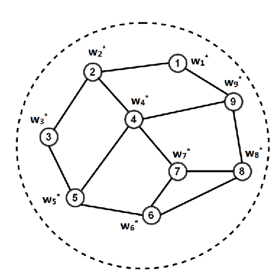
where wk⋆\textbf{w}^{\star}_{k} is an unknown optimal parameter vector to be estimated at node kk and ϵk​(n)\epsilon_{k}(n) is an observation noise with variance ξ0\xi^{0} which is assumed to be zero mean white noise and also independent of uk​(n)u_{k}(n) for all kk. Considering the number of parameter vectors to be estimated, which we shall refer to as the number of tasks, the distributed learning problem can be single-task or multi-task oriented. Therefore we distinguish among the following three types of networks, as illustrated by Fig. 1, depending on how the parameter vectors wk⋆\textbf{w}^{\star}_{k} are related across nodes:

Refer to caption
(a)

Refer to caption
(b)

Refer to caption
(c)
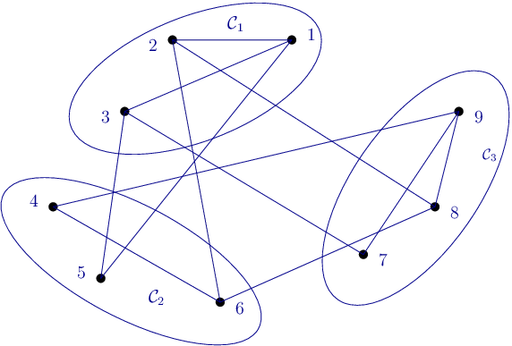
Figure 1: Three types of networks. Through direct links, nodes can communicate with each other in one hop. (a) Single-task Network. (b) Multi-task network. (c) Clustered multi-task network
  • •

    Single-task networks: All nodes in the network have to estimate the same parameter vector wk⋆\textbf{w}^{\star}_{k}. That is, in this case we have that

    w⋆k=w⋆,∀k∈1,2,…,N\begin{split}\textbf{w}^{\star}_{k}=\textbf{w}^{\star},\hskip 30.00005pt\forall k\in{1,2,...,N}\end{split} (2)
  • •

    Multi-task networks: Each node kk in the network has to determine its own optimum parameter vector, wk⋆\textbf{w}^{\star}_{k}. However, it is assumed that similarities and relationships exist among the parameters of neighboring nodes, which we denote by writing

    wk⋆∼wl⋆,i​fl∈𝒩k\begin{split}\textbf{w}^{\star}_{k}\sim\textbf{w}^{\star}_{l},\hskip 30.00005ptif\hskip 10.00002ptl\in\mathcal{N}_{k}\end{split} (3)

    The sign ∼\sim represents a similarity relationship in some sense, and its meaning will become clear soon once we introduce expression (8) and (9) further ahead. There are many situations in practice where the objective parameters are not identical across clusters but have inherent relationships. It is therefore beneficial to exploit these relationships to enhance performance. Here we focus on promoting the similarity of objective parameter vectors via their distance to each other.

  • •

    Clustered Multi-task Networks: Nodes are grouped into Q clusters, and there is one task per cluster. The optimum parameter vectors are only constrained to be equal within each cluster. The optimum parameter vectors are only constrained to be equal within each cluster, but similarities between neighboring clusters are allowed to exist, namely,

    wk⋆=w𝒞q⋆,wheneverk∈𝒞qw𝒞p⋆∼w𝒞q⋆,if𝒞p,𝒞q​are connected\begin{split}\textbf{w}^{\star}_{k}=\textbf{w}^{\star}_{\mathcal{C}_{q}},\hskip 30.00005pt\text{whenever}\hskip 10.00002ptk\in\mathcal{C}_{q}\hskip 28.00006pt\\ \textbf{w}^{\star}_{\mathcal{C}_{p}}\sim\textbf{w}^{\star}_{\mathcal{C}_{q}},\hskip 30.00005pt\text{if}\hskip 10.00002pt\mathcal{C}_{p},\mathcal{C}_{q}\hskip 5.0pt\text{are connected}\end{split} (4)

    where pp and qq denote two cluster indexes. We say that two clusters 𝒞p\mathcal{C}_{p} and 𝒞p\mathcal{C}_{p} are connected if there exists at least one edge linking a node from one cluster to a node in the other cluster.

One can observe that the single-task and multi-task networks are particular cases of the clustered multi-task network. In the case where all nodes are clustered together, the clustered multi-task network reduces to the single-task network. on the other hand, in the case where each cluster only involves one node, the clustered multi-task network becomes a multi-task network. Building on the literature on diffusion strategies for single-task networks, we shall now generalize its usage and analysis for distributed learning over clustered multi-task networks. These results will also be applicable to multi-task networks by setting the number of clusters equal to the number of nodes.

III Problem Formulation

In clustered multitask networks the nodes that are grouped into cluster estimate the same coefficient vector. Thus, consider the cluster 𝒞⁡(k)\mathcal{C}(k) to which node kk belongs. Under certain settings, in order to provide independence from the input data correlation statistics, we introduce normalized updates with respect to the input regressor at each node uk​(n)\textbf{u}_{k}(n). A local cost function, Jk​(w𝒞⁡(k))J_{k}(\textbf{w}_{\mathcal{C}(k)}), is associated with node kk and it is assumed that the Hessian matrix of the cost function is positive semi-definite. The local cost function Jk​(w𝒞⁡(k))J_{k}(\textbf{w}_{\mathcal{C}(k)}) is defined as

Jk​(w𝒞⁡(k))=E⁡{|dk​(n)−ukT​(n)​w𝒞k‖uk​(n)‖|2}\begin{split}J_{k}(\textbf{w}_{\mathcal{C}(k)})=E\{|\frac{\textbf{d}_{k}(n)-\textbf{u}^{T}_{k}(n)\textbf{w}_{\mathcal{C}_{k}}}{\|\textbf{u}_{k}(n)\|}|^{2}\}\end{split} (5)

Depending on the application, there may be certain properties among the optimal vectors {w𝒞1∗,…,{w𝒞Q∗}\{\textbf{w}^{*}_{\mathcal{C}_{1}},\ldots,\{\textbf{w}^{*}_{\mathcal{C}_{Q}}\}. This Mutual information among tasks could be used to improve the estimation accuracy. Among the possible options, a simple yet effective, Euclidian distance based regularizer was enforced in [18]. The squared Euclidean distance regularizer is given as

Δ⁡(w𝒞k,w𝒞l)=‖w𝒞k−w𝒞l‖2\begin{split}\Delta(\textbf{w}_{\mathcal{C}_{k}},\textbf{w}_{\mathcal{C}_{l}})=\|\textbf{w}_{\mathcal{C}_{k}}-\textbf{w}_{\mathcal{C}_{l}}\|^{2}\end{split} (6)

To estimate the unknown parameter vectors {w𝒞1∗,…,{w𝒞Q∗}\{\textbf{w}^{*}_{\mathcal{C}_{1}},\ldots,\{\textbf{w}^{*}_{\mathcal{C}_{Q}}\}, it was shown in [18] that the local cost (5) and the regularizer (6) can be combined at the level of each cluster. This formulation led to the following estimation problem defined in terms of QQ Nash equilibrium problems [20], where each cluster 𝒞j\mathcal{C}_{j} estimates w𝒞j∗\textbf{w}^{*}_{\mathcal{C}_{j}} by minimizing the regularized cost function J𝒞j​(w𝒞j,w−𝒞j)J_{\mathcal{C}_{j}}(\textbf{w}_{\mathcal{C}_{j}},\textbf{w}_{-\mathcal{C}_{j}}):

(𝒫1)​{minw𝒞j⁡J𝒞j​(w𝒞j,w−𝒞j)with​J𝒞j​(w𝒞j,w−𝒞j)=∑k∈𝒞jE⁡{|dk​(n)−ukT​(n)​w𝒞k‖uk​(n)‖|2}+η​∑k∈𝒞j∑l∈𝒩k∖𝒞jρk​l​‖w𝒞k−w𝒞l‖2\begin{split}(\mathcal{P}_{1})\begin{cases}\min\limits_{\textbf{w}_{\mathcal{C}_{j}}}J_{\mathcal{C}_{j}}(\textbf{w}_{\mathcal{C}_{j}},\textbf{w}_{-\mathcal{C}_{j}})\\ \text{with}\hskip 1.99997ptJ_{\mathcal{C}_{j}}(\textbf{w}_{\mathcal{C}_{j}},\textbf{w}_{-\mathcal{C}_{j}})=\sum\limits_{k\in\mathcal{C}_{j}}E\{|\frac{\textbf{d}_{k}(n)-\textbf{u}^{T}_{k}(n)\textbf{w}_{\mathcal{C}_{k}}}{\|\textbf{u}_{k}(n)\|}|^{2}\}+\eta\sum\limits_{k\in\mathcal{C}_{j}}\sum\limits_{l\in\mathcal{N}_{k}\setminus\mathcal{C}_{j}}\rho_{kl}\|\textbf{w}_{\mathcal{C}_{k}}-\textbf{w}_{\mathcal{C}_{l}}\|^{2}\end{cases}\end{split} (7)

for j=1,…,Qj=1,\ldots,Q. w𝒞j​(n)\textbf{w}_{\mathcal{C}_{j}}(n) is the parameter vector associated with cluster 𝒞j\mathcal{C}_{j}, η>0\eta>0 is a regularization parameter, and the symbol ∖\setminus is the set difference. Note that we have kept the notation w𝒞k\textbf{w}_{\mathcal{C}_{k}} in above equation to make the role of the regularization term clearer, even though we have w𝒞⁡(k)=w𝒞j\textbf{w}_{\mathcal{C}(k)}=\textbf{w}_{\mathcal{C}_{j}} for all kk in 𝒞j\mathcal{C}_{j}. The notation w−𝒞j\textbf{w}_{-\mathcal{C}_{j}} denotes the collection of weight vectors estimated by the other clusters, that is, w−𝒞j={w𝒞q;q=1,…,Q}−{w𝒞j}\textbf{w}_{-\mathcal{C}_{j}}=\{\textbf{w}_{\mathcal{C}_{q}};q=1,\ldots,Q\}-\{\textbf{w}_{\mathcal{C}_{j}}\}. The non-negative coefficients ρk​l\rho_{kl} aim at the adjusting the regularization strength. In [18]. The coefficients {ρk​l}\{\rho_{kl}\} were chosen to satisfy the conditions:

∑l∈𝒩k∖𝒞⁡(k)ρk​l=1,and​{ρk​l>0,ifl∈𝒩k∖𝒞(k),ρk​k≥0,ρk​l=0,otherwise\begin{split}\sum\limits_{l\in\mathcal{N}_{k}\setminus\mathcal{C}(k)}\rho_{kl}=1,\text{and}\hskip 3.00003pt\begin{cases}\rho_{kl}>0,\text{if}\hskip 3.00003ptl\in\mathcal{N}_{k}\setminus\mathcal{C}(k),\\ \rho_{kk}\geq 0,\\ \rho_{kl}=0,\text{otherwise}\end{cases}\end{split} (8)

We impose ρk​l=0\rho_{kl}=0 for all l∉Nk∖C⁡(k)l\notin N_{k}\setminus C(k), since nodes belonging to the same cluster estimate the same parameter vector.

The solution for the problem 𝒫1\mathcal{P}_{1} requires that every node in the network should have the access to the statistical moments Ru,k\textbf{R}_{u,k} and pu​d,k\textbf{p}_{ud,k} over its cluster, however, node kk can only be assumed to have direct access to the information from its neighborhood 𝒩k\mathcal{N}_{k}, which may include the nodes that are not part of the cluster 𝒞⁡(k)\mathcal{C}(k) Therefore, to enable a distributed solution that relies only on measured data from neighborhood, as mentioned in [18], [19] the cost function is relaxed into following form:

J𝒞⁡(k)​(wk)=∑l∈𝒩k∩𝒞⁡(k)cl​k​E​{|dl​(n)−ulT​(n)​wk‖uk​(n)‖|2}+η​∑l∈𝒩k∖𝒞⁡(k)ρk​l​‖wk−wl‖2+∑l∈𝒩k−∩𝒞⁡(k)bl​k∥wk−wol∥2\begin{split}J_{\mathcal{C}(k)}(\textbf{w}_{k})&=\sum\limits_{l\in\mathcal{N}_{k}\cap\mathcal{C}(k)}c_{lk}E\{|\frac{\textbf{d}_{l}(n)-\textbf{u}^{T}_{l}(n)\textbf{w}_{k}}{\|\textbf{u}_{k}(n)\|}|^{2}\}+\eta\sum\limits_{l\in\mathcal{N}_{k}\setminus\mathcal{C}(k)}\rho_{kl}\|\textbf{w}_{k}-\textbf{w}_{l}\|^{2}\\ &+\sum\limits_{l\in\mathcal{N}^{-}_{k}\cap\mathcal{C}(k)}b_{lk}\|\textbf{w}_{k}-\textbf{w}^{o}_{l}\|^{2}\end{split} (9)

where the coefficients cl​kc_{lk} are non-negative and satisfy the conditions:

∑k=1Ncl​k=1,and​cl​k=0​if​k∉𝒩l∩𝒞⁡(l)\begin{split}\sum\limits_{k=1}^{N}c_{lk}=1,\hskip 3.00003pt\text{and}\hskip 6.99997ptc_{lk}=0\hskip 6.99997pt\text{if}\hskip 3.00003ptk\notin\mathcal{N}_{l}\cap\mathcal{C}(l)\end{split} (10)

and the coefficients bl​kb_{lk} are also non-negative.

Following the same line of reasoning from [10],[11]\cite[cite]{[\@@bibref{}{10}{}{}]},\cite[cite]{[\@@bibref{}{11}{}{}]} in the single-task case, and extending the argument to problem (9) by using Nash-equilibrium properties [20], and by following same procedure mentioned in [10], [21] the following diffusion strategy of the adapt-then-combine (ATC) for clustered multi-task Normalized LMS (NLMS) is derived in distributed manner:

{𝝍k​(n+1)=wk​(n)+μ​uk​(n)‖ε+uk​(n)‖2​[dk​(n)−ukT​(n)​wk​(n)]+μk​η​∑l∈𝒩k∖𝒞⁡(k)ρk​l​(wl​(n)−wk​(n))wk​(n+1)=∑l∈𝒩k∩𝒞⁡(k)al​k​𝝍l​(n+1)\begin{split}\begin{cases}\boldsymbol{\psi}_{k}(n+1)=\textbf{w}_{k}(n)+\mu\frac{\textbf{u}_{k}(n)}{\|\varepsilon+\textbf{u}_{k}(n)\|^{2}}[\textbf{d}_{k}(n)-\textbf{u}^{T}_{k}(n)\textbf{w}_{k}(n)]+\mu_{k}\eta\hskip 5.0pt\sum\limits_{l\in\mathcal{N}_{k}\setminus\mathcal{C}(k)}{}\rho_{kl}(\textbf{w}_{l}(n)-\textbf{w}_{k}(n))\\ \textbf{w}_{k}(n+1)=\sum\limits_{l\in\mathcal{N}_{k}\cap\mathcal{C}(k)}{}a_{lk}\hskip 1.99997pt\boldsymbol{\psi}_{l}(n+1)\\ \end{cases}\end{split} (11)

By extending the above clustered multi-task diffusion strategy to data-reuse case, we can derive the following Affine projection algorithm (APA) [22] based clustered multi-task diffusion strategy:

{𝝍k​(n+1)=wk​(n)+μ​UkT​(n)​(ε​I+Uk​(n)​UkT​(n))−1​[dk​(n)−uk​(n)​wk​(n)]+μk​η∑l∈𝒩k∖𝒞⁡(k)ρk​l​(wl​(n)−wk​(n))wk​(n+1)=∑l∈𝒩k∩𝒞⁡(k)al​k​𝝍l​(n+1)\begin{split}\begin{cases}\boldsymbol{\psi}_{k}(n+1)&=\textbf{w}_{k}(n)+\mu\textbf{U}^{T}_{k}(n)\left(\varepsilon I+\textbf{U}_{k}(n)\textbf{U}^{T}_{k}(n)\right)^{-1}[\textbf{d}_{k}(n)-\textbf{u}_{k}(n)\textbf{w}_{k}(n)]\\ &\hskip 20.00003pt+\mu_{k}\hskip 1.99997pt\eta\hskip 10.00002pt\sum\limits_{l\in\mathcal{N}_{k}\setminus\mathcal{C}(k)}{}\rho_{kl}(\textbf{w}_{l}(n)-\textbf{w}_{k}(n))\\ \textbf{w}_{k}(n+1)&=\sum\limits_{l\in\mathcal{N}_{k}\cap\mathcal{C}(k)}{}a_{lk}\hskip 1.99997pt\boldsymbol{\psi}_{l}(n+1)\\ \end{cases}\end{split} (12)

where η\eta denotes a regularization parameter with small positive value, ε\varepsilon is employed to avoid the inversion of a rank deficient matrix Uk​(n)​UkT​(n)\textbf{U}_{k}(n)\textbf{U}^{T}_{k}(n) and the input data matrix Uk​(n)\textbf{U}_{k}(n), desired response vector dk​(n)\textbf{d}_{k}(n) are given as follows

Uk​(n)=[uk​(n)uk​(n−1)⋮uk​(n−P+1)],dk​(n)=[dk​(n)dk​(n−1)⋮dk​(n−P+1)]\begin{split}\textbf{U}_{k}(n)=\left[\begin{array}[]{c}\textbf{u}_{k}(n)\\ \textbf{u}_{k}(n-1)\\ \vdots\\ \textbf{u}_{k}(n-P+1)\end{array}\right],\hskip 20.00003pt\textbf{d}_{k}(n)=\left[\begin{array}[]{c}d_{k}(n)\\ d_{k}(n-1)\\ \vdots\\ d_{k}(n-P+1)\end{array}\right]\end{split} (13)

The clustered multi-task diffusion APA algorithm is given below:

Algorithm 1 Diffusion APA for clustered multi-task networks
0:  Start wk​(0)=0\textbf{w}_{k}(0)=0 for all kk, and repeat:
𝝍k​(n+1)=wk​(n)+μk​UkT​(n)​(ε​I+Uk​(n)​UkT​(n))−1​[dk​(n)−Uk​(n)​wk​(n)]+μkη∑l∈𝒩k∖𝒞⁡(k)ρk​l(wl(n)−wk(n))wk​(n+1)=∑l∈𝒩k∩𝒞⁡(k)al​k​𝝍l​(n+1)\begin{split}\boldsymbol{\psi}_{k}(n+1)&=\textbf{w}_{k}(n)+\mu_{k}\hskip 1.99997pt\textbf{U}^{T}_{k}(n)\left(\varepsilon I+\textbf{U}_{k}(n)\textbf{U}^{T}_{k}(n)\right)^{-1}[\textbf{d}_{k}(n)-\textbf{U}_{k}(n)\textbf{w}_{k}(n)]\\ &\hskip 46.00012pt+\hskip 1.99997pt\mu_{k}\hskip 1.99997pt\eta\hskip 1.99997pt\sum\limits_{l\in\mathcal{N}_{k}\setminus\mathcal{C}(k)}{}\rho_{kl}(\textbf{w}_{l}(n)-\textbf{w}_{k}(n))\\ \textbf{w}_{k}(n+1)&=\sum\limits_{l\in\mathcal{N}_{k}\cap\mathcal{C}(k)}{}a_{lk}\hskip 3.00003pt\boldsymbol{\psi}_{l}(n+1)\end{split} (14)

In a single-task network, there is a single cluster that consists of the entire set of nodes we get 𝒩k∩𝒞⁡(k)=𝒩k\mathcal{N}_{k}\cap\mathcal{C}(k)=\mathcal{N}_{k} and 𝒩k∖𝒞⁡(k)=∅\mathcal{N}_{k}\setminus\mathcal{C}(k)=\emptyset for all kk, so that the expression (14) reduces to the diffusion adaptation strategy [10] as described in algorithm 22:

Algorithm 2 Diffusion APA for single-task networks
0:  Start wk​(0)=0\textbf{w}_{k}(0)=0 for all kk, and repeat:
𝝍k​(n+1)=wk​(n)+μk​UkT​(n)​(ε​I+Uk​(n)​UkT​(n))−1​[dk​(n)−Uk​(n)​wk​(n)]wk​(n+1)=∑l∈𝒩kal​k​𝝍l​(n+1)\begin{split}\boldsymbol{\psi}_{k}(n+1)&=\textbf{w}_{k}(n)+\mu_{k}\hskip 1.99997pt\textbf{U}^{T}_{k}(n)\left(\varepsilon I+\textbf{U}_{k}(n)\textbf{U}^{T}_{k}(n)\right)^{-1}[\textbf{d}_{k}(n)-\textbf{U}_{k}(n)\textbf{w}_{k}(n)]\\ \textbf{w}_{k}(n+1)&=\sum\limits_{l\in\mathcal{N}_{k}}{}a_{lk}\hskip 3.00003pt\boldsymbol{\psi}_{l}(n+1)\end{split} (15)

In the case of multi-task network where the size of each cluster is one, we have 𝒩k∩𝒞⁡(k)=k\mathcal{N}_{k}\cap\mathcal{C}(k)={k} and 𝒩k∖𝒞⁡(k)=𝒩k−\mathcal{N}_{k}\setminus\mathcal{C}(k)=\mathcal{N}^{-}_{k} for all kk. Then algorithm 11 degenerates into Algorithm 33. This is the instantaneous gradient counterpart of (14) for each node.

Algorithm 3 Diffusion APA for multi-task networks
0:  Start wk​(0)=0\textbf{w}_{k}(0)=0 for all kk, and repeat:
wk​(n+1)=wk​(n)+μk​UkT​(n)​(ε​I+Uk​(n)​UkT​(n))−1​[dk​(n)−Uk​(n)​wk​(n)]+μkη∑l∈𝒩k−ρk​l(wl(n)−wk(n))\begin{split}\textbf{w}_{k}(n+1)=\textbf{w}_{k}(n)&+\mu_{k}\hskip 1.99997pt\textbf{U}^{T}_{k}(n)\left(\varepsilon I+\textbf{U}_{k}(n)\textbf{U}^{T}_{k}(n)\right)^{-1}[\textbf{d}_{k}(n)-\textbf{U}_{k}(n)\textbf{w}_{k}(n)]\\ &+\hskip 1.99997pt\mu_{k}\hskip 1.99997pt\eta\hskip 1.99997pt\sum\limits_{l\in\mathcal{N}^{-}_{k}}{}\rho_{kl}(\textbf{w}_{l}(n)-\textbf{w}_{k}(n))\\ \end{split} (16)

IV Mean-Square Error Performance Analysis

IV-A Network Global Model

The space-time structure of the algorithm leads to challenge in the performance analysis. To proceed, first, Let us define the global representations as

𝝍⁡(n)=col​{𝝍1​(n),𝝍2​(n),…,𝝍N​(n)},w​(n)=col​{w1​(n),w2​(n),…,wN​(n)}U​(n)=diag​{U1​(n),U2​(n),…,UN​(n)},d​(n)=col​{d1​(n),d2​(n),…,dN​(n)}\begin{split}\boldsymbol{\psi}(n)&=\text{col}\{\boldsymbol{\psi}_{1}(n),\boldsymbol{\psi}_{2}(n),\ldots,\boldsymbol{\psi}_{N}(n)\},\hskip 10.00002pt\textbf{w}(n)=\text{col}\{\textbf{w}_{1}(n),\textbf{w}_{2}(n),\ldots,\textbf{w}_{N}(n)\}\\ \textbf{U}(n)&=\text{diag}\{\textbf{U}_{1}(n),\textbf{U}_{2}(n),\ldots,\textbf{U}_{N}(n)\},\hskip 10.00002pt\textbf{d}(n)=\text{col}\{\textbf{d}_{1}(n),\textbf{d}_{2}(n),\ldots,\textbf{d}_{N}(n)\}\\ \end{split} (17)

where U​(n)\textbf{U}(n) is an N​M×L​NNM\times LN block diagonal matrix. The L​N×L​NLN\times LN diagonal matrices D and 𝜼\boldsymbol{\eta} are defined as

D=diag​{μ1​IL,μ2​IL,…,μN​IL}𝜼=diag​{η1​IL,η2​IL,…,ηN​IL}\begin{split}\textbf{D}&=\text{diag}\{\mu_{1}\textbf{I}_{L},\mu_{2}\textbf{I}_{L},\ldots,\mu_{N}\textbf{I}_{L}\}\\ \boldsymbol{\eta}&=\text{diag}\{\eta_{1}\textbf{I}_{L},\eta_{2}\textbf{I}_{L},\ldots,\eta_{N}\textbf{I}_{L}\}\end{split} (18)

to collect the local step-sizes and regularization parameters. From the linear model of the form (1),\eqref{eq2.1}, the global model at network level is obtained as

d​(n)=U​(n)​w⋆+v​(n)\begin{split}\textbf{d}(n)=\textbf{U}(n)\textbf{w}^{\star}+\textbf{\emph{v}}(n)\end{split} (19)

where w⋆​(n)\textbf{w}^{\star}(n) and v​(n)\textbf{v}(n) are global optimal weight and noise vectors given as follows

w⋆​(n)=col​{w1⋆​(n),w2⋆​(n),…,wN⋆​(n)}v​(n)=col​{v1​(n),v2​(n),…,vN​(n)}\begin{split}\textbf{w}^{\star}(n)&=\text{col}\{\textbf{w}^{\star}_{1}(n),\textbf{w}^{\star}_{2}(n),\ldots,\textbf{w}^{\star}_{N}(n)\}\\ \textbf{\emph{v}}(n)&=\text{col}\{\textbf{\emph{v}}_{1}(n),\textbf{\emph{v}}_{2}(n),\ldots,\textbf{\emph{v}}_{N}(n)\}\end{split} (20)

To facilitate analysis, the network topology is assumed to be static (i.e. al​k​(n)=al​ka_{lk}(n)=a_{lk}). This assumption does not compromise the algorithm derivation or its operation, and is used for analysis only. The analysis presented in [23] and [24] serves as the basis for this work. Using the above expressions, the global model of multi-task diffusion APA is therefore formulated as follows:

w​(n+1)=𝓐⁡[w​(n)+D​UT​(n)​[ε​I+U​(n)​UT​(n)]−1​[d​(n)−U​(n)​w​(n)]−D​𝜼​𝓠​w​(n)]\begin{split}\textbf{w}(n+1)&=\boldsymbol{\mathcal{A}}\hskip 1.99997pt\Big[\textbf{w}(n)+\textbf{D}\hskip 1.99997pt\textbf{U}^{T}(n)\big[\varepsilon\textbf{I}+\textbf{U}(n)\textbf{U}^{T}(n)\big]^{-1}\hskip 5.0pt[\textbf{d}(n)-\textbf{U}(n)\textbf{w}(n)]\hskip 1.99997pt-\textbf{D}\hskip 1.00006pt\boldsymbol{\eta}\hskip 1.99997pt\boldsymbol{\mathcal{Q}}\hskip 1.99997pt\textbf{w}(n)\Big]\end{split} (21)

where

𝓐=AT⊗IL𝓠=IL​N−P⊗IL\begin{split}\boldsymbol{\mathcal{A}}&=\textbf{A}^{T}\otimes\textbf{I}_{L}\\ \boldsymbol{\mathcal{Q}}&=\textbf{I}_{LN}-\textbf{P}\otimes\textbf{I}_{L}\end{split} (22)

with ⊗\otimes denoting the Kronecker product, A is the N×NN\times N symmetric matrix that defines the network topology and P is the N×NN\times N asymmetric matrix that defines regularizer strength among the nodes with ρk​k=1\rho_{kk}=1 if 𝒩k∖𝒞⁡(k)\mathcal{N}_{k}\setminus\mathcal{C}(k). Now the objective is to study the performance behavior of the multi-task diffusion APA governed by the form (21).

IV-B Mean Error Behavior Analysis

The global error vector e​(n)\textbf{e}(n) is related to the local error vectors ek​(n)\textbf{e}_{k}(n) as

e​(n)=col​{e1​(n),e2​(n),…,eN​(n)}\begin{split}\textbf{e}(n)&=\text{col}\{\textbf{e}_{1}(n),\textbf{e}_{2}(n),\ldots,\textbf{e}_{N}(n)\}\end{split} (23)

By denoting w~​(n)=w⋆−w​(n)\widetilde{\textbf{w}}(n)=\textbf{w}^{\star}-\textbf{w}(n), the global weight error vector can be rewritten as

e(n)=[d(n)−U(n)w(n)]]=U(n)w~(n)+v(n)=ea(n)+v(n)\begin{split}\textbf{e}(n)=[\textbf{d}(n)-\textbf{U}(n)\textbf{w}(n)]\hskip 1.99997pt\Big]=\textbf{U}(n)\widetilde{\textbf{w}}(n)+\textbf{\emph{v}}(n)=\textbf{e}_{a}(n)+\textbf{\emph{v}}(n)\end{split} (24)

where

ea​(n)=U​(n)​w~​(n)\begin{split}\textbf{e}_{a}(n)=\textbf{U}(n)\widetilde{\textbf{w}}(n)\end{split} (25)

Using these results the recursive update equation of global weight error vector can be written as

w~​(n+1)=𝓐⁡[w~​(n)−D​UT​(n)​[ε​I+U​(n)​UT​(n)]−1​U​(n)​w~​(n)−D​UT​(n)​[ε​I+U​(n)​UT​(n)]−1​v​(n)−D​𝜼​𝓠​[w~​(n)−w⋆]]=𝓐⁡[IL​N−D​Z​(n)−D​𝜼​𝓠]​w~​(n)−AI​D​UT​(n)​[ε​I+U​(n)​UT​(n)]−1​v​(n)+𝓐​D​𝜼​𝓠​w⋆\begin{split}\widetilde{\textbf{w}}(n+1)&=\boldsymbol{\mathcal{A}}\hskip 1.99997pt\Big[\widetilde{\textbf{w}}(n)-\textbf{D}\hskip 1.00006pt\textbf{U}^{T}(n)\big[\varepsilon\textbf{I}+\textbf{U}(n)\textbf{U}^{T}(n)\big]^{-1}\hskip 1.00006pt\textbf{U}(n)\widetilde{\textbf{w}}(n)\hskip 1.00006pt-\textbf{D}\hskip 1.00006pt\textbf{U}^{T}(n)\big[\varepsilon\textbf{I}+\textbf{U}(n)\textbf{U}^{T}(n)\big]^{-1}\hskip 1.00006pt\textbf{\emph{v}}(n)-\hskip 1.00006pt\textbf{D}\hskip 1.00006pt\boldsymbol{\eta}\hskip 1.99997pt\boldsymbol{\mathcal{Q}}\big[\widetilde{\textbf{w}}(n)-\textbf{w}^{\star}\big]\Big]\\ &=\boldsymbol{\mathcal{A}}\hskip 1.99997pt\Big[\textbf{I}_{LN}-\textbf{D}\hskip 1.99997pt\textbf{Z}(n)\hskip 1.99997pt-\hskip 1.99997pt\textbf{D}\hskip 1.99997pt\boldsymbol{\eta}\hskip 1.99997pt\boldsymbol{\mathcal{Q}}\Big]\hskip 1.99997pt\widetilde{\textbf{w}}(n)-\textbf{A}_{I}\hskip 1.00006pt\textbf{D}\hskip 1.00006pt\textbf{U}^{T}(n)\big[\varepsilon\textbf{I}+\textbf{U}(n)\textbf{U}^{T}(n)\big]^{-1}\hskip 1.00006pt\textbf{\emph{v}}(n)+\boldsymbol{\mathcal{A}}\hskip 1.99997pt\textbf{D}\hskip 1.99997pt\boldsymbol{\eta}\hskip 1.99997pt\boldsymbol{\mathcal{Q}}\hskip 1.99997pt\textbf{w}^{\star}\\ \end{split} (26)

where Z​(n)=UT​(n)​[ε​I+U​(n)​UT​(n)]−1​U​(n)\textbf{Z}(n)=\textbf{U}^{T}(n)\big[\varepsilon\textbf{I}+\textbf{U}(n)\textbf{U}^{T}(n)\big]^{-1}\hskip 1.00006pt\textbf{U}(n). Taking the expectation E⁡[⋅]E[\cdot] on both sides, and using the statistical independence between wk​(n)\textbf{w}_{k}(n) and Uk​(n)\textbf{U}_{k}(n) (i.e., “independence assumption”), and recalling that vk​(n)\textbf{v}_{k}(n) is zero-mean i.i.d and also independent of Uk​(n)\textbf{U}_{k}(n) and thus of wk​(n)\textbf{w}_{k}(n) we can write

E⁡[w~​(n+1)]=𝓐⁡[IL​N−D​E​[Z​(n)]−D​𝜼​𝓠]​E​[w~​(n)]+𝓐​D​𝜼​𝓠​w⋆\begin{split}E\big[\widetilde{\textbf{w}}(n+1)\big]=\boldsymbol{\mathcal{A}}\bigg[\textbf{I}_{LN}-\textbf{D}\hskip 1.99997ptE\big[\textbf{Z}(n)\big]\hskip 1.99997pt-\hskip 1.99997pt\textbf{D}\hskip 1.99997pt\boldsymbol{\eta}\hskip 1.99997pt\boldsymbol{\mathcal{Q}}\bigg]E[\widetilde{\textbf{w}}(n)]+\boldsymbol{\mathcal{A}}\hskip 1.99997pt\textbf{D}\hskip 1.99997pt\boldsymbol{\eta}\hskip 1.99997pt\boldsymbol{\mathcal{Q}}\hskip 1.99997pt\textbf{w}^{\star}\end{split} (27)

Then, for any initial condition, in order to guarantee the stability of the multi-task diffusion APA strategy in the mean sense, the step size μk\mu_{k} has to be chosen to satisfy

λm​a​x​(𝓐⁡[IL​N−D​Z¯−D​𝜼​𝓠])<1\begin{split}\lambda_{max}\Big(\hskip 1.00006pt\boldsymbol{\mathcal{A}}\big[\textbf{I}_{LN}-\textbf{D}\hskip 1.99997pt\overline{\textbf{Z}}-\textbf{D}\hskip 1.99997pt\boldsymbol{\eta}\hskip 1.99997pt\boldsymbol{\mathcal{Q}}\big]\hskip 1.00006pt\Big)<1\end{split} (28)

where Z¯=E​[Z​(n)]\overline{\textbf{Z}}=E[\textbf{Z}(n)], and λm​a​x​(⋅)\lambda_{max}(\cdot) denotes the maximum eigen value of its argument matrix. Therefore, using the norm inequalities and recalling the fact that the combining matrix A is a left stochastic matrix ( i.e., block maximum norm is equal to one), we have

‖𝓐⁡[IL​N−D​Z¯−D​𝜼​𝓠]‖b,∞≤‖[IL​N−D​Z¯−D​𝜼​𝓠]‖b,∞≤‖[IL​N−D​Z¯−D​𝜼+D​𝜼​(P⊗IL)]‖b,∞\begin{split}\|\boldsymbol{\mathcal{A}}\big[\textbf{I}_{LN}-\textbf{D}\hskip 1.99997pt\overline{\textbf{Z}}-\textbf{D}\hskip 1.99997pt\boldsymbol{\eta}\hskip 1.99997pt\boldsymbol{\mathcal{Q}}\big]\|_{b,\infty}&\leq\|\big[\textbf{I}_{LN}-\textbf{D}\hskip 1.99997pt\overline{\textbf{Z}}-\textbf{D}\hskip 1.99997pt\boldsymbol{\eta}\hskip 1.99997pt\boldsymbol{\mathcal{Q}}\big]\|_{b,\infty}\\ &\leq\|\big[\textbf{I}_{LN}-\textbf{D}\hskip 1.99997pt\overline{\textbf{Z}}-\textbf{D}\hskip 1.99997pt\boldsymbol{\eta}\hskip 1.99997pt+\textbf{D}\hskip 1.99997pt\boldsymbol{\eta}\hskip 1.99997pt\big(\textbf{P}\otimes\textbf{I}_{L}\big)\big]\|_{b,\infty}\end{split} (29)

Let AA be the an L×LL\times L matrix, then from Gershgorin circle theorem, we have:

|λ−ai,i|≤∑j≠i|ai,j||\lambda-a_{i,i}|\leq\sum\limits_{j\neq i}|a_{i,j}| (30)

Therefore, using the above result, and recalling the fact that P is a right stochastic matrix, a sufficient condition for (29) to hold is to choose μ\mu such that

0<μk<2maxk​{λm​a​x​(Z¯k)}+2​η\begin{split}0<\mu_{k}<\frac{2}{\text{max}_{k}\{\lambda_{max}(\hskip 1.99997pt\overline{\textbf{Z}}_{k})\}+2\eta}\end{split} (31)

where Z¯k=E⁡[UkT​(n)​[ε​I+Uk​(n)​UkT​(n)]−1​Uk​(n)]\overline{\textbf{Z}}_{k}=E\Big[\textbf{U}_{k}^{T}(n)\big[\varepsilon\textbf{I}+\textbf{U}_{k}(n)\textbf{U}_{k}^{T}(n)\big]^{-1}\hskip 5.0pt\textbf{U}_{k}(n)\Big]. Above result clearly shows that the mean stability limit of the clustered multi-task diffusion APA is lower than the diffusion APA due to the presence of η\eta.

In steady-state i.e., as n→∞n\rightarrow\infty the asymptotic mean bias is given by

limn→∞E⁡[w~​(n)]=[IL​N−𝓐⁡[IL​N−D​Z¯−D​𝜼​𝓠]]−1​𝓐​D ​𝜼​𝓠​w⋆\begin{split}\lim\limits_{n\to\infty}E\big[\widetilde{\textbf{w}}(n)\big]=\Bigg[\textbf{I}_{LN}-\boldsymbol{\mathcal{A}}\hskip 1.99997pt\bigg[\textbf{I}_{LN}-\textbf{D}\hskip 1.99997pt\overline{\textbf{Z}}\hskip 1.99997pt-\hskip 1.99997pt\textbf{D}\hskip 1.99997pt\boldsymbol{\eta}\hskip 1.99997pt\boldsymbol{\mathcal{Q}}\bigg]\Bigg]^{-1}\boldsymbol{\mathcal{A}}\hskip 1.99997pt\textbf{D }\hskip 1.99997pt\boldsymbol{\eta}\hskip 1.99997pt\boldsymbol{\mathcal{Q}}\hskip 1.99997pt\textbf{w}^{\star}\end{split} (32)

IV-C Mean-Square Error Behavior Analysis

The recursive update equation of weight error vector can also be rewritten as follows:

w~​(n+1)=𝓖⁡(n)​w~​(n)−𝓐​D​UT​(n)​[ε​I+U​(n)​UT​(n)]−1​v​(n)+r\begin{split}\widetilde{\textbf{w}}(n+1)&=\boldsymbol{\mathcal{G}}(n)\hskip 3.00003pt\widetilde{\textbf{w}}(n)-\boldsymbol{\mathcal{A}}\hskip 1.99997pt\textbf{D}\hskip 1.00006pt\textbf{U}^{T}(n)\big[\varepsilon\textbf{I}+\textbf{U}(n)\textbf{U}^{T}(n)\big]^{-1}\textbf{\emph{v}}(n)+\textbf{r}\end{split} (33)

where

𝓖⁡(n)=𝓐⁡[IL​N−D​Z​(n)−D​𝜼​𝓠]r=𝓐​D​𝜼​𝓠​w⋆\begin{split}\boldsymbol{\mathcal{G}}(n)&=\boldsymbol{\mathcal{A}}\hskip 1.99997pt\Big[\textbf{I}_{LN}-\textbf{D}\hskip 1.99997pt\textbf{Z}(n)-\textbf{D}\hskip 1.99997pt\boldsymbol{\eta}\hskip 1.00006pt\boldsymbol{\mathcal{Q}}\Big]\\ \textbf{r}&=\boldsymbol{\mathcal{A}}\hskip 1.99997pt\textbf{D}\hskip 1.99997pt\boldsymbol{\eta}\hskip 1.99997pt\boldsymbol{\mathcal{Q}}\hskip 1.99997pt\textbf{w}^{\star}\end{split} (34)

Using the standard independent assumption between Uk​(n)\textbf{U}_{k}(n) and wk​(n)\textbf{w}_{k}(n) and E​[v​(n)]=0E[\textbf{v}(n)]=0, the mean square of the weight error vector w~​(n+1)\widetilde{\textbf{w}}(n+1), weighted by any positive semi-definite matrix 𝚺\boldsymbol{\Sigma} that we are free to choose, satisfies the following relation:

E​‖w~​(n+1)‖𝚺2=E∥w~(n)∥E𝚺′2+E[vT(n)Y𝚺(n)v(n)]+E[w~T(n)]E[𝓖T(n)]𝚺r+rT𝚺E[𝓖(n)]E[w~(n)]+∥r∥𝚺2\begin{split}E\|\widetilde{\textbf{w}}(n+1)\|_{\boldsymbol{\Sigma}}^{2}&=E\|\widetilde{\textbf{w}}(n)\|_{E\boldsymbol{\Sigma}^{{}^{\prime}}}^{2}+E\big[\textbf{\emph{v}}^{T}(n)\hskip 1.00006pt\textbf{Y}^{\boldsymbol{\Sigma}}(n)\hskip 1.00006pt\textbf{\emph{v}}(n)\big]+E\big[\widetilde{\textbf{w}}^{T}(n)\big]\hskip 1.99997ptE\big[\boldsymbol{\mathcal{G}}^{T}(n)\big]\hskip 1.00006pt\boldsymbol{\Sigma}\hskip 1.99997pt\textbf{r}+\textbf{r}^{T}\hskip 1.99997pt\boldsymbol{\Sigma}\hskip 1.99997ptE\big[\boldsymbol{\mathcal{G}}(n)\big]\hskip 1.99997ptE\big[\widetilde{\textbf{w}}(n)\big]+\|\textbf{r}\|_{\boldsymbol{\Sigma}}^{2}\end{split} (35)

where

E𝚺′=E⁡[𝓖T​(n)​𝚺​𝓖​(n)]=𝓐T​𝚺​𝓐−E⁡[Z​(n)]​D​𝓐T​𝚺​𝓐−𝓐T​𝚺​𝓐​D​E​[Z​(n)]−𝓐T​𝚺​S−ST​𝚺​𝓐+E⁡[Z​(n)]​D​𝓐IT​𝚺​S+ST​𝚺​𝓐​D​E​[Z​(n)]+E⁡[UT​(n)​Y𝚺​U​(n)]+ST​𝚺​S\begin{split}E\boldsymbol{\Sigma}^{{}^{\prime}}&=E\Big[\boldsymbol{\mathcal{G}}^{T}(n)\hskip 1.99997pt\boldsymbol{\Sigma}\hskip 1.99997pt\boldsymbol{\mathcal{G}}(n)\Big]\\ &=\hskip 1.99997pt\boldsymbol{\mathcal{A}}^{T}\hskip 1.00006pt\boldsymbol{\Sigma}\hskip 1.99997pt\boldsymbol{\mathcal{A}}-E\big[\textbf{Z}(n)]\hskip 1.99997pt\textbf{D}\hskip 1.00006pt\boldsymbol{\mathcal{A}}^{T}\hskip 1.00006pt\boldsymbol{\Sigma}\hskip 1.00006pt\boldsymbol{\mathcal{A}}-\boldsymbol{\mathcal{A}}^{T}\hskip 1.00006pt\boldsymbol{\Sigma}\hskip 1.00006pt\boldsymbol{\mathcal{A}}\hskip 1.00006pt\textbf{D}\hskip 1.00006ptE\big[\textbf{Z}(n)\big]-\boldsymbol{\mathcal{A}}^{T}\hskip 1.00006pt\boldsymbol{\Sigma}\hskip 1.00006pt\textbf{S}-\textbf{S}^{T}\hskip 1.00006pt\boldsymbol{\Sigma}\hskip 1.00006pt\boldsymbol{\mathcal{A}}\hskip 1.00006pt\\ &\hskip 1.99997pt+E\big[\textbf{Z}(n)\big]\textbf{D}\hskip 1.00006pt\boldsymbol{\mathcal{A}}^{T}_{I}\hskip 1.00006pt\boldsymbol{\Sigma}\hskip 1.00006pt\textbf{S}+\textbf{S}^{T}\hskip 1.00006pt\boldsymbol{\Sigma}\hskip 1.00006pt\boldsymbol{\mathcal{A}}\hskip 1.00006pt\textbf{D}\hskip 1.00006ptE\big[\textbf{Z}(n)\big]+E\big[\textbf{U}^{T}(n)\hskip 1.00006pt\textbf{Y}^{\boldsymbol{\Sigma}}\hskip 1.00006pt\textbf{U}(n)\big]+\textbf{S}^{T}\hskip 1.00006pt\boldsymbol{\Sigma}\hskip 1.99997pt\textbf{S}\end{split} (36)

and

Y𝚺=[ε​I+U​(n)​UT​(n)]−1​U​(n)​D​𝓐T​𝚺​𝓐​D​UT​(n)​[ε​I+U​(n)​UT​(n)]−1S=𝓐​D​𝜼​𝓠\begin{split}\textbf{Y}^{\boldsymbol{\Sigma}}&=\big[\varepsilon\textbf{I}+\textbf{U}(n)\textbf{U}^{T}(n)\big]^{-1}\textbf{U}(n)\hskip 1.99997pt\textbf{D}\hskip 1.99997pt\boldsymbol{\mathcal{A}}^{T}\hskip 1.99997pt\boldsymbol{\Sigma}\hskip 1.99997pt\boldsymbol{\mathcal{A}}\hskip 1.99997pt\textbf{D}\hskip 1.99997pt\textbf{U}^{T}(n)\big[\varepsilon\textbf{I}+\textbf{U}(n)\textbf{U}^{T}(n)\big]^{-1}\\ \textbf{S}&=\boldsymbol{\mathcal{A}}\hskip 1.99997pt\textbf{D}\hskip 1.99997pt\boldsymbol{\eta}\hskip 1.99997pt\boldsymbol{\mathcal{Q}}\end{split} (37)

In order to study the behavior of the multi-task diffusion APA algorithm, the following moments in (35) and (36) must be evaluated:

E⁡[Z​(n)​D​𝓐T​𝚺​𝓐​D​Z​(n)]E⁡[vT​(n)​[ε​I+U​(n)​UT​(n)]−1​U​(n)​D​𝓐T​𝚺​𝓐​D​UT​(n)​[ε​I+U​(n)​UT​(n)]−1​v​(n)]\begin{split}&E\Big[\textbf{Z}(n)\hskip 1.99997pt\textbf{D}\hskip 1.99997pt\boldsymbol{\mathcal{A}}^{T}\hskip 1.99997pt\boldsymbol{\Sigma}\hskip 1.99997pt\boldsymbol{\mathcal{A}}\hskip 1.99997pt\textbf{D}\hskip 1.99997pt\textbf{Z}(n)\Big]\\ &E\Big[\textbf{\emph{v}}^{T}(n)\big[\varepsilon\textbf{I}+\textbf{U}(n)\textbf{U}^{T}(n)\big]^{-1}\textbf{U}(n)\hskip 1.99997pt\textbf{D}\hskip 1.99997pt\boldsymbol{\mathcal{A}}^{T}\hskip 1.99997pt\boldsymbol{\Sigma}\hskip 1.99997pt\boldsymbol{\mathcal{A}}\hskip 1.99997pt\textbf{D}\hskip 1.99997pt\textbf{U}^{T}(n)\big[\varepsilon\textbf{I}+\textbf{U}(n)\textbf{U}^{T}(n)\big]^{-1}\textbf{\emph{v}}(n)\Big]\end{split} (38)

To extract the matrix 𝚺\boldsymbol{\Sigma} from the expectation terms, a weighted variance relation is introduced by using L2​N2×1L^{2}N^{2}\times 1 column vectors:

𝝈=bvec{𝚺}and𝝈′=bvec{E𝚺′}\begin{split}\boldsymbol{\sigma}=\text{bvec}\{\boldsymbol{\Sigma}\}\hskip 20.00003pt\text{and}\hskip 20.00003pt\boldsymbol{\sigma^{{}^{\prime}}}=\text{bvec}\{E\boldsymbol{\Sigma}^{{}^{\prime}}\}\end{split} (39)

where bvec​{⋅}\text{bvec}\{\cdot\} denotes the block vector operator. In addition, bvec​{⋅}\text{bvec}\{\cdot\} is also used to recover the original matrix Σ\Sigma from 𝝈\boldsymbol{\sigma}. One property of the bvec​{⋅}\text{bvec}\{\cdot\} operator when working with the block Kronecker product [26] is used in this work, namely,

bvec​{Q​𝚺​P}=(PT⊗bQ)​𝝈\begin{split}\text{bvec}\{\textbf{Q}\boldsymbol{\Sigma}\textbf{P}\}=(\textbf{P}^{T}\otimes_{b}\textbf{Q})\hskip 1.99997pt\boldsymbol{\sigma}\end{split} (40)

where P⊗bQ\textbf{P}\otimes_{b}\textbf{Q} denotes the block Kronecker product [25], [26] of two block matrices.

Using (40) to (36) after block vectorization, the following terms on the right side of (36) are given by

bvec​{𝓐T​𝚺​𝓐}=(𝓐T⊗b𝓐T)​𝝈\begin{split}\text{bvec}\Big\{\boldsymbol{\mathcal{A}}^{T}\hskip 1.99997pt\boldsymbol{\Sigma}\hskip 1.99997pt\boldsymbol{\mathcal{A}}\Big\}&=\Big(\boldsymbol{\mathcal{A}}^{T}\otimes_{b}\boldsymbol{\mathcal{A}}^{T}\Big)\hskip 1.99997pt\boldsymbol{\sigma}\end{split} (41)
bvec​{E⁡[Z​(n)]​D​𝓐T​𝚺​𝓐}=(IL​N⊗bE⁡[Z​(n)])​(IL​N⊗bD)​(𝓐T⊗b𝓐T)​𝝈\begin{split}\text{bvec}\Big\{E\big[\textbf{Z}(n)\big]\hskip 1.99997pt\textbf{D}\hskip 1.99997pt\boldsymbol{\mathcal{A}}^{T}\boldsymbol{\Sigma}\hskip 1.99997pt\boldsymbol{\mathcal{A}}\Big\}&=\Big(\textbf{I}_{LN}\otimes_{b}E\big[\textbf{Z}(n)\big]\Big)\hskip 1.99997pt\Big(\textbf{I}_{LN}\otimes_{b}\textbf{D}\Big)\hskip 1.99997pt\Big(\boldsymbol{\mathcal{A}}^{T}\otimes_{b}\boldsymbol{\mathcal{A}}^{T}\Big)\hskip 1.99997pt\boldsymbol{\sigma}\end{split} (42)
bvec​{𝓐T​𝚺​𝓐​D​E​[Z​(n)]}=(E⁡[Z​(n)]⊗bIL​N)​(D⊗bIL​N)​(𝓐T⊗b𝓐T)​𝝈\begin{split}\text{bvec}\Big\{\boldsymbol{\mathcal{A}}^{T}\boldsymbol{\Sigma}\hskip 1.99997pt\boldsymbol{\mathcal{A}}\hskip 1.99997pt\textbf{D}\hskip 1.99997ptE[\textbf{Z}(n)]\Big\}&=\Big(E\big[\textbf{Z}(n)\big]\otimes_{b}\textbf{I}_{LN}\Big)\Big(\textbf{D}\otimes_{b}\textbf{I}_{LN}\Big)\Big(\boldsymbol{\mathcal{A}}^{T}\otimes_{b}\boldsymbol{\mathcal{A}}^{T}\Big)\hskip 1.99997pt\boldsymbol{\sigma}\end{split} (43)
bvec​{𝓐T​𝚺​S}=bvec​{𝓐T​𝚺​𝓐​D​𝜼​𝓠}=(𝓠T⊗bIL​N)​(𝜼⊗bIL​N)​(D⊗bIL​N)​(𝓐T⊗b𝓐T)​𝝈\begin{split}\text{bvec}\Big\{\boldsymbol{\mathcal{A}}^{T}\hskip 1.99997pt\boldsymbol{\Sigma}\hskip 1.99997pt\textbf{S}\Big\}&=\text{bvec}\Big\{\boldsymbol{\mathcal{A}}^{T}\hskip 1.99997pt\boldsymbol{\Sigma}\hskip 1.99997pt\boldsymbol{\mathcal{A}}\hskip 1.99997pt\textbf{D}\hskip 1.99997pt\boldsymbol{\eta}\hskip 1.99997pt\boldsymbol{\mathcal{Q}}\Big\}\\ &=\Big(\boldsymbol{\mathcal{Q}}^{T}\otimes_{b}\textbf{I}_{LN}\Big)\Big(\boldsymbol{\eta}\otimes_{b}\textbf{I}_{LN}\Big)\Big(\textbf{D}\otimes_{b}\textbf{I}_{LN}\Big)\Big(\boldsymbol{\mathcal{A}}^{T}\otimes_{b}\boldsymbol{\mathcal{A}}^{T}\Big)\hskip 1.99997pt\boldsymbol{\sigma}\end{split} (44)
bvec​{ST​𝚺​𝓐}=bvec​{𝓠T​𝜼​D​𝓐T​𝚺​𝓐}=(IL​N⊗b𝓠T)​(IL​N⊗b𝜼)​(IL​N⊗bD)​(𝓐T⊗b𝓐T)​𝝈\begin{split}\text{bvec}\Big\{\textbf{S}^{T}\hskip 1.99997pt\boldsymbol{\Sigma}\hskip 1.99997pt\boldsymbol{\mathcal{A}}\Big\}&=\text{bvec}\Big\{\boldsymbol{\mathcal{Q}}^{T}\hskip 1.99997pt\boldsymbol{\eta}\hskip 1.99997pt\textbf{D}\hskip 1.99997pt\boldsymbol{\mathcal{A}}^{T}\hskip 1.99997pt\boldsymbol{\Sigma}\hskip 1.99997pt\boldsymbol{\mathcal{A}}\Big\}\\ &=\Big(\textbf{I}_{LN}\otimes_{b}\boldsymbol{\mathcal{Q}}^{T}\Big)\Big(\textbf{I}_{LN}\otimes_{b}\boldsymbol{\eta}\Big)\Big(\textbf{I}_{LN}\otimes_{b}\textbf{D}\Big)\Big(\boldsymbol{\mathcal{A}}^{T}\otimes_{b}\boldsymbol{\mathcal{A}}^{T}\Big)\hskip 1.99997pt\boldsymbol{\sigma}\end{split} (45)
bvec​{E⁡[Z​(n)]​D​𝓐T​𝚺​S}=bvec​{E⁡[Z​(n)]​D​𝓐T​Σ​𝓐​D​𝜼​𝓠}=(IL​N⊗bE⁡[Z​(n)])​(𝓠T⊗bIL​N)​(𝜼⊗bIL​N)​(D⊗bD)​(𝓐T⊗b𝓐)​𝝈\begin{split}\text{bvec}\Big\{E\big[\textbf{Z}(n)\big]\hskip 1.99997pt\textbf{D}\hskip 1.99997pt\boldsymbol{\mathcal{A}}^{T}\boldsymbol{\Sigma}\hskip 1.99997pt\textbf{S}\Big\}&=\text{bvec}\Big\{E\big[\textbf{Z}(n)\big]\hskip 1.99997pt\textbf{D}\hskip 1.99997pt\boldsymbol{\mathcal{A}}^{T}\Sigma\hskip 1.99997pt\boldsymbol{\mathcal{A}}\hskip 1.99997pt\textbf{D}\hskip 1.99997pt\boldsymbol{\eta}\hskip 1.99997pt\boldsymbol{\mathcal{Q}}\Big\}\\ &=\Big(\textbf{I}_{LN}\otimes_{b}E\big[\textbf{Z}(n)\big]\Big)\Big(\boldsymbol{\mathcal{Q}}^{T}\otimes_{b}\textbf{I}_{LN}\Big)\Big(\boldsymbol{\eta}\otimes_{b}\textbf{I}_{LN}\Big)\Big(\textbf{D}\otimes_{b}\textbf{D}\Big)\Big(\boldsymbol{\mathcal{A}}^{T}\otimes_{b}\boldsymbol{\mathcal{A}}\Big)\hskip 1.99997pt\boldsymbol{\sigma}\end{split} (46)
bvec​{ST​𝚺​𝓐​D​E​[Z​(n)]}=bvec​{𝓠T​𝜼​D​𝓐T​𝚺​𝓐​D​E​[Z​(n)]}=(E⁡[Z​(n)]⊙IL​N)​(IL​N⊗b𝓠T)​(IL​N⊗b𝜼)​(D⊗bD)​(𝓐T⊗b𝓐T)​𝝈\begin{split}\text{bvec}\Big\{\textbf{S}^{T}\boldsymbol{\Sigma}\hskip 1.99997pt\boldsymbol{\mathcal{A}}\hskip 1.99997pt\textbf{D}\hskip 1.99997ptE\big[\textbf{Z}(n)\big]\Big\}&=\text{bvec}\Big\{\boldsymbol{\mathcal{Q}}^{T}\hskip 1.99997pt\boldsymbol{\eta}\hskip 1.00006pt\textbf{D}\hskip 1.00006pt\boldsymbol{\mathcal{A}}^{T}\hskip 1.99997pt\boldsymbol{\Sigma}\hskip 1.99997pt\boldsymbol{\mathcal{A}}\hskip 1.99997pt\textbf{D}\hskip 1.99997ptE\big[\textbf{Z}(n)\big]\Big\}\\ &=\Big(E[\textbf{Z}(n)]\odot\textbf{I}_{LN}\Big)\Big(\textbf{I}_{LN}\otimes_{b}\boldsymbol{\mathcal{Q}}^{T}\Big)\Big(\textbf{I}_{LN}\otimes_{b}\boldsymbol{\eta}\Big)\Big(\textbf{D}\otimes_{b}\textbf{D}\Big)\Big(\boldsymbol{\mathcal{A}}^{T}\otimes_{b}\boldsymbol{\mathcal{A}}^{T}\Big)\hskip 1.99997pt\boldsymbol{\sigma}\end{split} (47)
bvec​{UT​(n)​Y𝚺​U​(n)}=bvec​{E⁡[Z​(n)​D​𝓐T​𝚺​𝓐​D​Z​(n)]}=E⁡[Z​(n)⊗bZ​(n)]​(D⊗bD)​(𝓐T⊗b𝓐T)​𝝈\begin{split}\text{bvec}\Big\{\textbf{U}^{T}(n)\textbf{Y}^{\boldsymbol{\Sigma}}\hskip 1.99997pt\textbf{U}(n)\Big\}&=\text{bvec}\Big\{E\big[\textbf{Z}(n)\hskip 1.99997pt\textbf{D}\hskip 1.99997pt\boldsymbol{\mathcal{A}}^{T}\hskip 1.99997pt\boldsymbol{\Sigma}\hskip 1.99997pt\boldsymbol{\mathcal{A}}\hskip 1.99997pt\textbf{D}\hskip 1.99997pt\textbf{Z}(n)\big]\Big\}\\ &=E\big[\textbf{Z}(n)\otimes_{b}\textbf{Z}(n)\big]\Big(\textbf{D}\otimes_{b}\textbf{D}\Big)\Big(\boldsymbol{\mathcal{A}}^{T}\otimes_{b}\boldsymbol{\mathcal{A}}^{T}\Big)\hskip 1.99997pt\boldsymbol{\sigma}\end{split} (48)
bvec​{ST​Σ​S}=bvec​{𝓠T​𝜼​D​𝓐T​𝚺​𝓐​D​𝜼​𝓠}=(𝓠T⊗b𝓠T)​(𝜼⊗b𝜼)​(D⊗bD)​(𝓐T⊗b𝓐T)​𝝈\begin{split}\text{bvec}\Big\{\textbf{S}^{T}\Sigma\hskip 1.99997pt\textbf{S}\Big\}&=\text{bvec}\Big\{\hskip 1.99997pt\boldsymbol{\mathcal{Q}}^{T}\boldsymbol{\eta}\hskip 1.99997pt\textbf{D}\hskip 1.99997pt\boldsymbol{\mathcal{A}}^{T}\boldsymbol{\Sigma}\hskip 1.99997pt\boldsymbol{\mathcal{A}}\hskip 1.99997pt\textbf{D}\hskip 1.99997pt\boldsymbol{\eta}\hskip 1.99997pt\boldsymbol{\mathcal{Q}}\Big\}\\ &=\Big(\boldsymbol{\mathcal{Q}}^{T}\otimes_{b}\boldsymbol{\mathcal{Q}}^{T}\Big)\Big(\boldsymbol{\eta}\otimes_{b}\boldsymbol{\eta}\Big)\Big(\textbf{D}\otimes_{b}\textbf{D}\Big)\Big(\boldsymbol{\mathcal{A}}^{T}\otimes_{b}\boldsymbol{\mathcal{A}}^{T}\Big)\hskip 1.99997pt\boldsymbol{\sigma}\end{split} (49)

Therefore, a linear relation between the corresponding vectors {𝝈,𝝈′}\{\boldsymbol{\sigma},\boldsymbol{\sigma}^{{}^{\prime}}\}is formulated by

𝝈′=F𝝈\begin{split}\boldsymbol{\sigma}^{{}^{\prime}}=\textbf{F}\boldsymbol{\sigma}\end{split} (50)

where F is an L2​N2×L2​N2L^{2}N^{2}\times L^{2}N^{2} matrix and given by

F=[IL​N−(IL​N⊗bZ¯)​(IL​N⊗bD)−(Z¯⊗bIL​N)​(D⊗bIL​N)−(𝓠T⊗bIL​N)​(𝜼⊗bIL​N)​(D⊗bIL​N)−(IL​N⊗b𝓠T)​(IL​N⊗b𝜼)​(IL​N⊗bD)+(IL​N⊗bZ¯)​(𝓠T⊗bIL​N)​(𝜼⊗bIL​N)​(D⊗bD)+(Z¯⊗bIL​N)​(IL​N⊗b𝓠T)​(IL​N⊗b𝜼)​(D⊗bD)+𝚷⁡(D⊗bD)+(𝓠T⊗b𝓠T)​(𝜼⊗b𝜼)​(D⊗bD)]​(𝓐T⊗b𝓐T)\begin{split}\textbf{F}&=\left[\begin{array}[]{l}\textbf{I}_{LN}-\big(\textbf{I}_{LN}\otimes_{b}\overline{\textbf{Z}}\big)\big(\textbf{I}_{LN}\otimes_{b}\textbf{D}\big)-\big(\overline{\textbf{Z}}\otimes_{b}\textbf{I}_{LN}\big)\big(\textbf{D}\otimes_{b}\textbf{I}_{LN}\big)\\ -\big(\boldsymbol{\mathcal{Q}}^{T}\otimes_{b}\textbf{I}_{LN}\big)\big(\boldsymbol{\eta}\otimes_{b}\textbf{I}_{LN}\big)\big(\textbf{D}\otimes_{b}\textbf{I}_{LN}\big)-\big(\textbf{I}_{LN}\otimes_{b}\boldsymbol{\mathcal{Q}}^{T}\big)\big(\textbf{I}_{LN}\otimes_{b}\boldsymbol{\eta}\big)\big(\textbf{I}_{LN}\otimes_{b}\textbf{D}\big)\\ +\big(\textbf{I}_{LN}\otimes_{b}\overline{\textbf{Z}}\big)\big(\boldsymbol{\mathcal{Q}}^{T}\otimes_{b}\textbf{I}_{LN}\big)\big(\boldsymbol{\eta}\otimes_{b}\textbf{I}_{LN}\big)\big(\textbf{D}\otimes_{b}\textbf{D}\big)\\ +\big(\overline{\textbf{Z}}\otimes_{b}\textbf{I}_{LN}\big)\big(\textbf{I}_{LN}\otimes_{b}\boldsymbol{\mathcal{Q}}^{T}\big)\big(\textbf{I}_{LN}\otimes_{b}\boldsymbol{\eta}\big)\big(\textbf{D}\otimes_{b}\textbf{D}\big)+\boldsymbol{\Pi}\big(\textbf{D}\otimes_{b}\textbf{D}\big)\\ +\big(\boldsymbol{\mathcal{Q}}^{T}\otimes_{b}\boldsymbol{\mathcal{Q}}^{T}\big)\big(\boldsymbol{\eta}\otimes_{b}\boldsymbol{\eta}\big)\big(\textbf{D}\otimes_{b}\textbf{D}\big)\end{array}\right]\big(\boldsymbol{\mathcal{A}}^{T}\otimes_{b}\boldsymbol{\mathcal{A}}^{T}\big)\end{split} (51)

where 𝚷=E⁡[Z​(n)⊗bZ​(n)]\boldsymbol{\Pi}=E\Big[\textbf{Z}(n)\otimes_{b}\textbf{Z}(n)\Big] Let Λv=E⁡[v​(n)​vT​(n)]\Lambda_{v}=E[\textbf{\emph{v}}(n)\textbf{\emph{v}}^{T}(n)] denote a N​M×N​MNM\times NM diagonal matrix, whose entries are the noise variances σv,k2\sigma^{2}_{v,k} for k=1,2,⋯,Nk=1,2,\cdots,N and given by

Λv=diag​{σv,12​IM,σv,22​IM,⋯,σv,N2​IM}\begin{split}\Lambda_{v}=\text{diag}\{\sigma^{2}_{v,1}\textbf{I}_{M},\sigma^{2}_{v,2}\textbf{I}_{M},\cdots,\sigma^{2}_{v,N}\textbf{I}_{M}\}\end{split} (52)

Using the independence assumption of noise signals, the term E⁡[vT​(n)​Y𝚺​(n)​v​(n)]E\big[\textbf{\emph{v}}^{T}(n)\hskip 1.00006pt\textbf{Y}^{\boldsymbol{\Sigma}}(n)\hskip 1.00006pt\textbf{\emph{v}}(n)\big] can be written as

E⁡[vT​(n)​Y𝚺​(n)​v​(n)]=T​r​(𝓐​D​E​[𝚽]​D​𝓐T​𝚺)=𝜸T​𝝈\begin{split}E\big[\textbf{\emph{v}}^{T}(n)\hskip 1.99997pt\textbf{Y}^{\boldsymbol{\Sigma}}(n)\hskip 1.99997pt\textbf{\emph{v}}(n)\big]&=Tr\Big(\boldsymbol{\mathcal{A}}\hskip 1.99997pt\textbf{D}\hskip 1.99997ptE[\boldsymbol{\Phi}]\hskip 1.99997pt\textbf{D}\hskip 1.99997pt\boldsymbol{\mathcal{A}}^{T}\boldsymbol{\Sigma}\Big)\\ &=\boldsymbol{\gamma}^{T}\hskip 1.99997pt\boldsymbol{\sigma}\end{split} (53)

where 𝚽=UT​(n)​[ε​I+U​(n)​UT​(n)]−1​𝚲v​(n)​[ε​I+U​(n)​UT​(n)]−1​U​(n)\boldsymbol{\Phi}=\textbf{U}^{T}(n)\big[\varepsilon\textbf{I}+\textbf{U}(n)\textbf{U}^{T}(n)\big]^{-1}\boldsymbol{\Lambda}_{v}(n)\big[\varepsilon\textbf{I}+\textbf{U}(n)\textbf{U}^{T}(n)\big]^{-1}\textbf{U}(n) and

𝜸=vec​{𝓐​D​E​[𝚽]​DT​𝓐T}=(𝓐⊗𝓐)​(D⊗D)​vec​{E⁡[WT​𝚲v​W]}=(𝓐⊗𝓐)​(D⊗D)​E​[(WT⊗WT)]​𝜸v\begin{split}\boldsymbol{\gamma}&=\text{vec}\big\{\boldsymbol{\mathcal{A}}\hskip 1.99997pt\textbf{D}E[\boldsymbol{\Phi}]\hskip 1.99997pt\textbf{D}^{T}\hskip 1.99997pt\boldsymbol{\mathcal{A}}^{T}\big\}\\ &=\big(\boldsymbol{\mathcal{A}}\otimes\boldsymbol{\mathcal{A}}\big)\big(\textbf{D}\otimes\textbf{D}\big)\text{vec}\big\{E[\textbf{W}^{T}\boldsymbol{\Lambda}_{v}\textbf{W}]\big\}\\ &=\big(\boldsymbol{\mathcal{A}}\otimes\boldsymbol{\mathcal{A}}\big)\big(\textbf{D}\otimes\textbf{D}\big)E\big[\big(\textbf{W}^{T}\otimes\textbf{W}^{T}\big)\big]\hskip 1.99997pt\boldsymbol{\gamma}_{v}\end{split} (54)

with W=[ε​I+U​(n)​UT​(n)]−1​U​(n)\textbf{W}=\big[\varepsilon\textbf{I}+\textbf{U}(n)\textbf{U}^{T}(n)\big]^{-1}\textbf{U}(n) and 𝜸v=vec​{𝚲v}\boldsymbol{\gamma}_{v}=\text{vec}\{\boldsymbol{\Lambda}_{v}\}.

Finally, let us define the f​(r,E​[w~​(n)],𝝈)\emph{\textbf{f}}\big(\textbf{r},E[\widetilde{\textbf{w}}(n)],\boldsymbol{\sigma}\big) as the last three terms on the right hand side of the (35), i.e,

f​(r,E​[w~​(n)],𝝈)=‖r‖𝚺2+E⁡[w~T​(n)]​E​[𝓖T​(n)]​𝚺​r+rT​𝚺​E​[𝓖⁡(n)]​E​[w~​(n)]\begin{split}\emph{\textbf{f}}\big(\textbf{r},E[\widetilde{\textbf{w}}(n)],\boldsymbol{\sigma}\big)&=\|\textbf{r}\|_{\boldsymbol{\Sigma}}^{2}+E\big[\widetilde{\textbf{w}}^{T}(n)\big]\hskip 1.99997ptE\big[\boldsymbol{\mathcal{G}}^{T}(n)\big]\hskip 1.99997pt\boldsymbol{\Sigma}\hskip 1.99997pt\textbf{r}+\textbf{r}^{T}\hskip 1.99997pt\boldsymbol{\Sigma}\hskip 1.99997ptE\big[\boldsymbol{\mathcal{G}}(n)\big]\hskip 1.00006ptE\big[\widetilde{\textbf{w}}(n)\big]\\ \end{split} (55)

Each term can be evaluated as follows. Now, let us consider the term E​‖r‖𝚺2E\|\textbf{r}\|_{\boldsymbol{\Sigma}}^{2}, that can be written

‖r‖𝚺2=(bvec​{𝓐​D​𝜼​𝓠​w⋆​(w⋆)T​𝓠T​𝜼​D​𝓐T})T​𝝈=rbT​𝝈\begin{split}\|\textbf{r}\|_{\boldsymbol{\Sigma}}^{2}&=\bigg(\text{bvec}\Big\{\boldsymbol{\mathcal{A}}\hskip 1.99997pt\textbf{D}\hskip 1.99997pt\boldsymbol{\eta}\hskip 1.99997pt\boldsymbol{\mathcal{Q}}\hskip 1.99997pt\textbf{w}^{\star}\big(\textbf{w}^{\star}\big)^{T}\boldsymbol{\mathcal{Q}}^{T}\boldsymbol{\eta}\hskip 1.99997pt\textbf{D}\hskip 1.99997pt\boldsymbol{\mathcal{A}}^{T}\Big\}\bigg)^{T}\hskip 1.99997pt\boldsymbol{\sigma}\\ &=\textbf{r}^{T}_{b}\boldsymbol{\sigma}\end{split} (56)

where

rb=E⁡(𝓐⊗b𝓐)​(D⊗bD)​(𝜼⊗b𝜼)​(𝓠⊗b𝓠)​bvec​{w⋆​(w⋆)T}\begin{split}\textbf{r}_{b}&=E\Big(\boldsymbol{\mathcal{A}}\otimes_{b}\boldsymbol{\mathcal{A}}\Big)\big(\textbf{D}\otimes_{b}\textbf{D}\big)\big(\boldsymbol{\eta}\otimes_{b}\boldsymbol{\eta}\big)\Big(\boldsymbol{\mathcal{Q}}\otimes_{b}\boldsymbol{\mathcal{Q}}\Big)\text{bvec}\Big\{\textbf{w}^{\star}\big(\textbf{w}^{\star}\big)^{T}\Big\}\\ \end{split} (57)

Consider the second term E⁡[w~T​(n)​𝓖T​(n)​𝚺​r]E\Big[\widetilde{\textbf{w}}^{T}(n)\hskip 1.99997pt\boldsymbol{\mathcal{G}}^{T}(n)\hskip 1.99997pt\boldsymbol{\Sigma}\hskip 3.00003pt\textbf{r}\Big] that can be simplified as follows:

E⁡[w~T​(n)​𝓖T​(n)​𝚺​r]=T​r​(E⁡[r​w~T​(n)​𝓖T​(n)]​𝚺)=𝜶1T​(n)​𝝈\begin{split}E\Big[\widetilde{\textbf{w}}^{T}(n)\hskip 1.99997pt\boldsymbol{\mathcal{G}}^{T}(n)\hskip 1.00006pt\boldsymbol{\Sigma}\hskip 3.00003pt\textbf{r}\Big]&=Tr\Big(E\Big[\textbf{r}\hskip 1.99997pt\widetilde{\textbf{w}}^{T}(n)\hskip 3.00003pt\boldsymbol{\mathcal{G}}^{T}(n)\Big]\hskip 1.99997pt\boldsymbol{\Sigma}\Big)\\ &=\boldsymbol{\alpha}^{T}_{1}(n)\hskip 1.99997pt\boldsymbol{\sigma}\end{split} (58)

where

𝜶1​(n)=(𝓐⊗b𝓐)​[(IL​N⊗bD)​(IL​N⊗b𝜼)​(IL​N⊗b𝓠)−(D⊗bD)​(IL​N⊗b𝜼)​(IL​N⊗b𝓠)​(Z¯⊗bIL​N)−(D⊗bD)​(𝜼⊗b𝜼)​(𝓠⊗b𝓠)]​bvec​{w⋆​E​[w~T​(n)]}\begin{split}\boldsymbol{\alpha}_{1}(n)&=\Big(\boldsymbol{\mathcal{A}}\otimes_{b}\boldsymbol{\mathcal{A}}\Big)\left[\begin{array}[]{l}\big(\textbf{I}_{LN}\otimes_{b}\textbf{D}\big)\big(\textbf{I}_{LN}\otimes_{b}\boldsymbol{\eta}\big)\Big(\textbf{I}_{LN}\otimes_{b}\boldsymbol{\mathcal{Q}}\Big)\\ -\big(\textbf{D}\otimes_{b}\textbf{D}\big)\big(\textbf{I}_{LN}\otimes_{b}\boldsymbol{\eta}\big)\Big(\textbf{I}_{LN}\otimes_{b}\boldsymbol{\mathcal{Q}}\Big)\big(\overline{\textbf{Z}}\otimes_{b}\textbf{I}_{LN}\big)\\ -\big(\textbf{D}\otimes_{b}\textbf{D}\big)\big(\boldsymbol{\eta}\otimes_{b}\boldsymbol{\eta}\big)\Big(\boldsymbol{\mathcal{Q}}\otimes_{b}\boldsymbol{\mathcal{Q}}\Big)\end{array}\right]\text{bvec}\Big\{\textbf{w}^{\star}E[\widetilde{\textbf{w}}^{T}(n)]\Big\}\\ \end{split} (59)

In the same way, third term E⁡[rT​𝚺​𝓖​(n)​w~​(n)]E\Big[\textbf{r}^{T}\hskip 3.00003pt\boldsymbol{\Sigma}\hskip 1.99997pt\boldsymbol{\mathcal{G}}(n)\hskip 1.99997pt\widetilde{\textbf{w}}(n)\Big] can be written as follows:

E⁡[rT​𝚺​𝓖​(n)​w~​(n)]=T​r​(E⁡[𝓖⁡(n)​w~​(n)​rT]​𝚺)=𝜶2T​(n)​𝝈\begin{split}E\Big[\textbf{r}^{T}\hskip 3.00003pt\boldsymbol{\Sigma}\hskip 1.99997pt\boldsymbol{\mathcal{G}}(n)\hskip 1.99997pt\widetilde{\textbf{w}}(n)\Big]&=Tr\Big(E\Big[\boldsymbol{\mathcal{G}}(n)\hskip 1.99997pt\widetilde{\textbf{w}}(n)\hskip 1.99997pt\textbf{r}^{T}\Big]\hskip 1.99997pt\boldsymbol{\Sigma}\Big)\\ &=\boldsymbol{\alpha}^{T}_{2}(n)\hskip 1.99997pt\boldsymbol{\sigma}\end{split} (60)

where

𝜶2​(n)=(𝓐⊗b𝓐)​[(D⊗bIL​N)​(𝜼⊗bIL​N)​(𝓠⊗bIL​N)−(D⊗bD)​(𝜼⊗bIL​N)​(𝓠⊗bIL​N)​(IL​N⊗bZ¯)−(D⊗bD)​(𝜼⊗b𝜼)​(𝓠⊗b𝓠)]​bvec​{E⁡[w~​(n)]​(w⋆)T}\begin{split}\boldsymbol{\alpha}_{2}(n)&=\Big(\boldsymbol{\mathcal{A}}\otimes_{b}\boldsymbol{\mathcal{A}}\Big)\left[\begin{array}[]{l}\big(\textbf{D}\otimes_{b}\textbf{I}_{LN}\big)\big(\boldsymbol{\eta}\otimes_{b}\textbf{I}_{LN}\big)\Big(\boldsymbol{\mathcal{Q}}\otimes_{b}\textbf{I}_{LN}\Big)\\ -\big(\textbf{D}\otimes_{b}\textbf{D}\big)\big(\boldsymbol{\eta}\otimes_{b}\textbf{I}_{LN}\big)\Big(\boldsymbol{\mathcal{Q}}\otimes_{b}\textbf{I}_{LN}\Big)\big(\textbf{I}_{LN}\otimes_{b}\overline{\textbf{Z}}\big)\\ -\big(\textbf{D}\otimes_{b}\textbf{D}\big)\big(\boldsymbol{\eta}\otimes_{b}\boldsymbol{\eta}\big)\Big(\boldsymbol{\mathcal{Q}}\otimes_{b}\boldsymbol{\mathcal{Q}}\Big)\end{array}\right]\text{bvec}\Big\{E[\widetilde{\textbf{w}}(n)]\big(\textbf{w}^{\star}\big)^{T}\Big\}\\ \end{split} (61)

Therefore, the mean-square behavior of the multi-task diffusion APA algorithm is summarized as follows:

E​‖w~​(n+1)‖𝝈2=E​‖w~​(n)‖F​𝝈2+𝜸T​𝝈+f​(r,E⁡[w~​(n)],𝝈)=E​‖w~​(n)‖F​𝝈2+𝜸T​𝝈+(rbT+𝜶1T​(n)+𝜶2T​(n))​𝝈\begin{split}E\|\widetilde{\textbf{w}}(n+1)\|_{\boldsymbol{\sigma}}^{2}&=E\|\widetilde{\textbf{w}}(n)\|_{\textbf{F}\boldsymbol{\sigma}}^{2}+\boldsymbol{\gamma}^{T}\hskip 1.00006pt\boldsymbol{\sigma}+\emph{\textbf{f}}\big(\textbf{r},E[\widetilde{\textbf{w}}(n)],\boldsymbol{\sigma}\big)\\ &=E\|\widetilde{\textbf{w}}(n)\|_{\textbf{F}\boldsymbol{\sigma}}^{2}+\boldsymbol{\gamma}^{T}\hskip 1.00006pt\boldsymbol{\sigma}+\Big(\textbf{r}^{T}_{b}+\boldsymbol{\alpha}^{T}_{1}(n)+\boldsymbol{\alpha}^{T}_{2}(n)\Big)\hskip 1.99997pt\boldsymbol{\sigma}\end{split} (62)

Therefore, the multi-task diffusion strategy presented in (14) is mean square stable if the matrix F is stable. Iterating the recursion (62) starting from n=0n=0, we get

E​‖w~​(n+1)‖𝝈2=E​‖w~​(0)‖Fn+1​𝝈2+𝜸T​∑i=0nFi​𝝈+∑i=0nf​(r,E⁡[w~​(n−i)],Fi​𝝈)\begin{split}E\|\widetilde{\textbf{w}}(n+1)\|_{\boldsymbol{\sigma}}^{2}&=E\|\widetilde{\textbf{w}}(0)\|_{\textbf{F}^{n+1}\boldsymbol{\sigma}}^{2}+\boldsymbol{\gamma}^{T}\hskip 1.00006pt\sum\limits_{i=0}^{n}\textbf{F}^{i}\boldsymbol{\sigma}+\sum\limits_{i=0}^{n}\emph{\textbf{f}}\big(\textbf{r},E[\widetilde{\textbf{w}}(n-i)],\textbf{F}^{i}\boldsymbol{\sigma}\big)\end{split} (63)

with initial condition w~​(0)=w⋆−w​(0)\widetilde{\textbf{w}}(0)=\textbf{w}^{\star}-\textbf{w}(0). If the matrix F is stable then the first and second terms in the above equation converge to a finite value as n→∞n\rightarrow\infty. Now, let us consider the third term on the RHS of the (63). We know that E​[w~​(n)]E[\widetilde{\textbf{w}}(n)] is uniformly bounded because (27) is a BIBO stable recursion with bounded driving term 𝓐​D​𝜼​𝓠​w⋆\hskip 1.99997pt\boldsymbol{\mathcal{A}}\hskip 1.99997pt\textbf{D}\hskip 1.99997pt\boldsymbol{\eta}\hskip 1.99997pt\boldsymbol{\mathcal{Q}}\hskip 1.99997pt\textbf{w}^{\star}. Therefore, from (55) f​(r,E⁡[w~​(n−i)],Fi​𝝈)\emph{\textbf{f}}\big(\textbf{r},E[\widetilde{\textbf{w}}(n-i)],\textbf{F}^{i}\boldsymbol{\sigma}\big) can be written as

f​(r,E⁡[w~​(n−i)],Fi​𝝈)=(rbT+𝜶1T​(n−i)+𝜶2T​(n−i))​Fi​𝝈\begin{split}\emph{\textbf{f}}\big(\textbf{r},E[\widetilde{\textbf{w}}(n-i)],\textbf{F}^{i}\boldsymbol{\sigma}\big)&=\Big(\textbf{r}^{T}_{b}+\boldsymbol{\alpha}^{T}_{1}(n-i)+\boldsymbol{\alpha}^{T}_{2}(n-i)\Big)\hskip 1.99997pt\textbf{F}^{i}\hskip 1.99997pt\boldsymbol{\sigma}\end{split} (64)

Provided that F is stable and there exist a matrix norm, denoted by ∥⋅∥p\|\cdot\|_{p} such that ‖F‖p=cp<1\|\textbf{F}\|_{p}=c_{p}<1. Applying this norm to f and using the matrix norms and triangular inequality, we can write ‖f​(r,E⁡[w~​(n−i)],Fi​𝝈)‖≤​v​cpi\|\emph{\textbf{f}}\big(\textbf{r},E[\widetilde{\textbf{w}}(n-i)],\textbf{F}^{i}\boldsymbol{\sigma}\big)\|\leq\emph{v}\hskip 1.00006ptc^{i}_{p}, given ​v\emph{v} is a small positive constant. Therefore E​‖w~​(n+1)‖𝝈2E\|\widetilde{\textbf{w}}(n+1)\|_{\boldsymbol{\sigma}}^{2} converges to a bounded value as n→∞n\rightarrow\infty, and the algorithm is said to be mean square stable.

By selecting 𝚺=1N​IL​N\boldsymbol{\Sigma}=\frac{1}{N}\textbf{I}_{LN} we can relate E​‖w~​(n+1)‖𝝈2E\|\widetilde{\textbf{w}}(n+1)\|_{\boldsymbol{\sigma}}^{2} and E​‖w~​(n)‖𝝈2E\|\widetilde{\textbf{w}}(n)\|_{\boldsymbol{\sigma}}^{2} as follows:

E​‖w~​(n+1)‖𝝈2=E​‖w~​(n)‖𝝈2+𝜸T​Fn​𝝈−E​‖w~​(0)‖(I(L​N)2−F)​Fn​𝝈2+∑i=0nf​(r,E⁡[w~​(n−i)],Fi​𝝈)−∑i=0n−1f(r,E[w~(n−1−i)],Fi𝝈)\begin{split}E\|\widetilde{\textbf{w}}(n+1)\|_{\boldsymbol{\sigma}}^{2}&=E\|\widetilde{\textbf{w}}(n)\|_{\boldsymbol{\sigma}}^{2}+\boldsymbol{\gamma}^{T}\textbf{F}^{n}\boldsymbol{\sigma}-E\|\widetilde{\textbf{w}}(0)\|_{\big(I_{(LN)^{2}}-\textbf{F}\hskip 0.81949pt\big)\textbf{F}^{n}\boldsymbol{\sigma}}^{2}+\sum\limits_{i=0}^{n}\emph{\textbf{f}}\big(\textbf{r},E[\widetilde{\textbf{w}}(n-i)],\textbf{F}^{i}\boldsymbol{\sigma}\big)\\ &\hskip 20.00003pt-\sum\limits_{i=0}^{n-1}\emph{\textbf{f}}\big(\textbf{r},E[\widetilde{\textbf{w}}(n-1-i)],\textbf{F}^{i}\boldsymbol{\sigma}\big)\end{split} (65)

we can rewrite the last two terms in the above equation as,

∑i=0nf​(r,E⁡[w~​(n−i)],Fi​𝝈)−∑i=0n−1f​(r,E⁡[w~​(n−1−i)],Fi​𝝈)=rbT​Fn​𝝈+[𝜶1T​(n)+𝜶2T​(n)+Γ⁡(n)]​𝝈\begin{split}&\sum\limits_{i=0}^{n}\emph{\textbf{f}}\big(\textbf{r},E[\widetilde{\textbf{w}}(n-i)],\textbf{F}^{i}\boldsymbol{\sigma}\big)-\sum\limits_{i=0}^{n-1}\emph{\textbf{f}}\big(\textbf{r},E[\widetilde{\textbf{w}}(n-1-i)],\textbf{F}^{i}\boldsymbol{\sigma}\big)=\textbf{r}_{b}^{T}\hskip 1.99997pt\textbf{F}^{n}\hskip 1.99997pt\boldsymbol{\sigma}+\left[\boldsymbol{\alpha}_{1}^{T}(n)+\boldsymbol{\alpha}_{2}^{T}(n)+\Gamma(n)\right]\hskip 1.99997pt\boldsymbol{\sigma}\end{split} (66)

where

𝚪⁡(n)=∑i=1n(𝜶1T​(n−i)+𝜶2T​(n−i))​Fi​𝝈−∑i=0n−1(𝜶1T​(n−1−i)+𝜶2T​(n−1−i))​Fi​𝝈\begin{split}\boldsymbol{\Gamma}(n)=\sum\limits_{i=1}^{n}\Big(\boldsymbol{\alpha}_{1}^{T}(n-i)+\boldsymbol{\alpha}_{2}^{T}(n-i)\Big)\textbf{F}^{i}\hskip 1.99997pt\boldsymbol{\sigma}-\sum\limits_{i=0}^{n-1}\Big(\boldsymbol{\alpha}_{1}^{T}(n-1-i)+\boldsymbol{\alpha}_{2}^{T}(n-1-i)\Big)\textbf{F}^{i}\hskip 1.99997pt\boldsymbol{\sigma}\end{split} (67)

Therefore, the recursion presented in (62) can be rewritten as,

E​‖w~​(n+1)‖𝝈2=E​‖w~​(n)‖𝝈2+𝜸T​Fn​𝝈−E​‖w~​(0)‖(I(L​N)2−F)​Fn​𝝈2+rbT​Fn​𝝈+[𝜶1T​(n)+𝜶2T​(n)+Γ⁡(n)]𝚪⁡(n+1)=𝚪⁡(n)​F+[[𝜶1T​(n)+𝜶2T​(n)]​[F−I(L​N)2]]\begin{split}E\|\widetilde{\textbf{w}}(n+1)\|_{\boldsymbol{\sigma}}^{2}&=E\|\widetilde{\textbf{w}}(n)\|_{\boldsymbol{\sigma}}^{2}+\boldsymbol{\gamma}^{T}\textbf{F}^{n}\boldsymbol{\sigma}-E\|\widetilde{\textbf{w}}(0)\|_{\big(I_{(LN)^{2}}-\textbf{F}\hskip 0.81949pt\big)\textbf{F}^{n}\boldsymbol{\sigma}}^{2}+\textbf{r}_{b}^{T}\textbf{F}^{n}\hskip 1.00006pt\boldsymbol{\sigma}+\left[\boldsymbol{\alpha}_{1}^{T}(n)+\boldsymbol{\alpha}_{2}^{T}(n)+\Gamma(n)\right]\\ \boldsymbol{\Gamma}(n+1)&=\boldsymbol{\Gamma}(n)\textbf{F}+\Big[\big[\boldsymbol{\alpha}_{1}^{T}(n)+\boldsymbol{\alpha}_{2}^{T}(n)\big]\hskip 1.99997pt[\textbf{F}-\textbf{I}_{(LN)^{2}}]\Big]\end{split} (68)

with 𝚪⁡(0)=01×(L​N)2\boldsymbol{\Gamma}(0)=0_{1\times(LN)^{2}}.

Steady-state MSD of the multi-task diffusion APA strategy is given as follows

limn→∞E​‖w~​(n)‖(I(L​N)2−F)​𝝈2=𝜸T​𝝈+f​(r,E⁡[w~​(∞)],𝝈)\begin{split}\lim\limits_{n\to\infty}E\|\widetilde{\textbf{w}}(n)\|_{\big(I_{(LN)^{2}}-\textbf{F}\big)\boldsymbol{\sigma}}^{2}&=\boldsymbol{\gamma}^{T}\boldsymbol{\sigma}+\emph{\textbf{f}}\big(\textbf{r},E[\widetilde{\textbf{w}}(\infty)],\boldsymbol{\sigma}\big)\end{split} (69)

IV-D New Approach to Improve the Performance of Clustered multi-task diffusion APA

Clustered multi-task diffusion strategy presented in (14) has mainly 22 drawbacks

  • •

    At time instance nn, assume that the node ll exhibiting poor performance over the node kk. The multi-task diffusion strategy forces the node kk to learn from node ll during the adaptation step where l∈Nk∖Ckl\in N_{k}\setminus C_{k}. This affects the performance in transient state.

  • •

    For all l∈Nk∖Ckl\in N_{k}\setminus C_{k} we have wk∗≃wl∗\textbf{w}_{k}^{*}\simeq\textbf{w}_{l}^{*} i.e, only the underlying system is same. However, the multitask diffusion strategy forces the node kk to learn from node ll even in the steady state. This hampers the steady state performance of the algorithm.

To address these problems a control variable called similarity measure, δk​l​(n)\delta_{kl}(n) is introduced to control the regularizer term in the multi-task diffusion strategy. At each time instance nn, node kk has access to its neighborhood filter coefficient vectors. Since the node is learning from its neighborhood filter coefficient vectors, it is reasonable to check the similarity among the filter coefficient vectors. The similarity measure is calculated as follows

δk​l​(n)=12​[1+s​i​g​n​(σk2​(n)−σk​l2​(n))]\begin{split}\delta_{kl}(n)=\frac{1}{2}\bigg[1+sign\Big(\hskip 1.99997pt\sigma^{2}_{k}(n)-\sigma^{2}_{kl}(n)\hskip 1.99997pt\Big)\bigg]\end{split} (70)

where σk2​(n)\sigma^{2}_{k}(n) and σl​k2​(n)\sigma^{2}_{lk}(n) are estimated error variances and can be calculated as

σk2​(n)=λ​σk2​(n−1)+(1−λ)​[dk​(n)−ukT​(n)​wk​(n)]2σk​l2​(n)=λσ2k​l(n−1)+(1−λ)[dk(n)−uTk(n)wl(n)]2forl∈𝒩k∖𝒞(k)\begin{split}\sigma^{2}_{k}(n)&=\lambda\hskip 1.99997pt\sigma^{2}_{k}(n-1)+(1-\lambda)\Big[d_{k}(n)-\textbf{u}^{T}_{k}(n)\textbf{w}_{k}(n)\Big]^{2}\\ \sigma^{2}_{kl}(n)&=\lambda\hskip 1.99997pt\sigma^{2}_{kl}(n-1)+(1-\lambda)\Big[d_{k}(n)-\textbf{u}^{T}_{k}(n)\textbf{w}_{l}(n)\Big]^{2}\hskip 10.00002pt\text{for}\hskip 10.00002ptl\in\mathcal{N}_{k}\setminus\mathcal{C}(k)\end{split} (71)

and λ\lambda is a positive constant with λ∈[0,1]\lambda\in[0,1].

To explain, suppose that at index nn, the node ll performs better than node kk, i.e., σk​l2​(n)<σk2​(n)\sigma^{2}_{kl}(n)<\sigma^{2}_{k}(n). Then for node kk the similarity measure δk​l​(n)=12​[1+s​i​g​n​(σk2​(n)−σk​l2​(n))]=1\delta_{kl}(n)=\frac{1}{2}\Big[1+sign\big(\hskip 1.99997pt\sigma^{2}_{k}(n)-\sigma^{2}_{kl}(n)\hskip 1.99997pt\big)\Big]=1, which implies that node kk would learn the weight information from node ll by adding the difference of their current weight vectors, i.e., [wl​(n)−wk​(n)][\textbf{w}_{l}(n)-\textbf{w}_{k}(n)] as a correction term to its weight update. On the other hand, suppose the node ll does not perform better than node kk, i.e., σk​l2​(n)>σk2​(n)\sigma^{2}_{kl}(n)>\sigma^{2}_{k}(n). Then for node kk the similarity measure δk​l​(n)=12​[1+s​i​g​n​(σk2​(n)−σk​l2​(n))]=0\delta_{kl}(n)=\frac{1}{2}\Big[1+sign\big(\hskip 1.99997pt\sigma^{2}_{k}(n)-\sigma^{2}_{kl}(n)\hskip 1.99997pt\big)\Big]=0, which implies that node kk would neglect the weight vector wl​(n)\textbf{w}_{l}(n). Thus improves the convergence rate and steady state performance over the multi-task diffusion strategy presented in (14).

Therefore, by taking the similarity measure, δk​l​(n)\delta_{kl}(n) into account the modified clustered multi-task diffusion APA is given below

𝝍k​(n+1)=wk​(n)+μk​UkT​(n)​(ε​I+Uk​(n)​UkT​(n))−1​[dk​(n)−UkT​(n)​wk​(n)]+μkη∑l∈𝒩k∖𝒞⁡(k)ρ′k​l(n)[wl(n)−wk(n)]wk​(n+1)=∑l∈𝒩k∩𝒞⁡(k)al​k​𝝍l​(n+1)\begin{split}\boldsymbol{\psi}_{k}(n+1)&=\textbf{w}_{k}(n)+\mu_{k}\hskip 3.00003pt\textbf{U}^{T}_{k}(n)\left(\varepsilon I+\textbf{U}_{k}(n)\textbf{U}^{T}_{k}(n)\right)^{-1}[\textbf{d}_{k}(n)-\textbf{U}^{T}_{k}(n)\textbf{w}_{k}(n)]\\ &\hskip 40.00006pt+\mu_{k}\hskip 1.99997pt\eta\sum\limits_{l\in\mathcal{N}_{k}\setminus\mathcal{C}(k)}{}\hskip 1.99997pt\rho^{{}^{\prime}}_{kl}(n)\hskip 1.99997pt\big[\textbf{w}_{l}(n)-\textbf{w}_{k}(n)\big]\\ \textbf{w}_{k}(n+1)&=\sum\limits_{l\in\mathcal{N}_{k}\cap\mathcal{C}(k)}{}a_{lk}\hskip 1.99997pt\boldsymbol{\psi}_{l}(n+1)\\ \end{split} (72)

where ρk​l′(n)=ρk​lδk​l(n)\rho^{{}^{\prime}}_{kl}(n)=\rho_{kl}\hskip 1.99997pt\delta_{kl}(n). Therefore, using the above expressions, the global model of modified multi-task diffusion APA is formulated as follows:

w​(n+1)=𝓐⁡[w​(n)+D​UT​(n)​[ε​I+U​(n)​UT​(n)]−1​e​(n)−D​𝜼​𝓠δ​(n)​w​(n)]\begin{split}\textbf{w}(n+1)&=\boldsymbol{\mathcal{A}}\hskip 1.99997pt\Big[\textbf{w}(n)+\textbf{D}\hskip 1.99997pt\textbf{U}^{T}(n)\big[\varepsilon\textbf{I}+\textbf{U}(n)\textbf{U}^{T}(n)\big]^{-1}\hskip 5.0pt\textbf{e}(n)\hskip 1.99997pt-\textbf{D}\hskip 1.99997pt\boldsymbol{\eta}\hskip 1.99997pt\boldsymbol{\mathcal{Q}}_{\delta}(n)\hskip 1.99997pt\textbf{w}(n)\Big]\end{split} (73)

where

𝓠δ​(n)=Dδ​(n)−Pδ​(n)⊗IL\begin{split}\boldsymbol{\mathcal{Q}}_{\delta}(n)&=\textbf{D}_{\delta}(n)-\textbf{P}_{\delta}(n)\otimes\textbf{I}_{L}\end{split} (74)

and

Dδ​(n)=diag​{δ1​(n)​IL​(n),δ2​(n)​IL​(n),⋯,δN​(n)​IL​(n)}\begin{split}\textbf{D}_{\delta}(n)&=\text{diag}\{\delta_{1}(n)\textbf{I}_{L}(n),\delta_{2}(n)\textbf{I}_{L}(n),\cdots,\delta_{N}(n)\textbf{I}_{L}(n)\}\\ \end{split} (75)

with

δk(n)=∑l∈𝒩k∖𝒞kρ′k​l(n)=∑l∈𝒩k∖𝒞kρk​lδk​l(n)\begin{split}\delta_{k}(n)=\sum\limits_{l\in\mathcal{N}_{k}\setminus\mathcal{C}_{k}}\rho^{{}^{\prime}}_{kl}(n)=\sum\limits_{l\in\mathcal{N}_{k}\setminus\mathcal{C}_{k}}\rho_{kl}\hskip 3.00003pt\delta_{kl}(n)\end{split} (76)

the matrix Pδ​(n)=P⊙𝜹⁡(n)\textbf{P}_{\delta}(n)=\textbf{P}\odot\boldsymbol{\delta}(n) (’⊙\odot’ indicates the Hadamard product) is the N×NN\times N asymmetric matrix that defines regularizer strength among the nodes with 𝜹k​(n)=1\boldsymbol{\delta}_{k}(n)=1 and Pδ,k​k​(n)=1\textbf{P}_{\delta,kk}(n)=1 if 𝒩k∖𝒞⁡(k)\mathcal{N}_{k}\setminus\mathcal{C}(k) is empty. The matrices 𝓐\boldsymbol{\mathcal{A}}, D, U​(n)\textbf{U}(n) are as same as the matrices defined in the network model section. Now the objective is to study the performance behavior of the multi-task diffusion APA governed by the form (73).

IV-E Mean Error Behavior Analysis

By denoting w~​(n)=w⋆−w​(n)\widetilde{\textbf{w}}(n)=\textbf{w}^{\star}-\textbf{w}(n) the recursive update equation of global weight error vector can be written as

w~​(n+1)=𝓐[IL​N−DZ(n)−D𝜼𝓠δ(n)]w~(n)−𝓐DUT(n)[εI+U(n)UT(n)]−1v(n)+𝓐D𝜼𝓠δ(n)w⋆\begin{split}\widetilde{\textbf{w}}(n+1)&=\boldsymbol{\mathcal{A}}\hskip 1.99997pt\Big[\textbf{I}_{LN}-\textbf{D}\hskip 1.99997pt\textbf{Z}(n)\hskip 1.99997pt-\hskip 1.99997pt\textbf{D}\hskip 1.99997pt\boldsymbol{\eta}\hskip 1.99997pt\boldsymbol{\mathcal{Q}}_{\delta}(n)\Big]\widetilde{\textbf{w}}(n)-\boldsymbol{\mathcal{A}}\hskip 1.00006pt\textbf{D}\hskip 1.00006pt\textbf{U}^{T}(n)\big[\varepsilon\textbf{I}+\textbf{U}(n)\textbf{U}^{T}(n)\big]^{-1}\hskip 1.00006pt\textbf{\emph{v}}(n)+\hskip 10.00002pt\boldsymbol{\mathcal{A}}\hskip 1.99997pt\textbf{D}\hskip 1.99997pt\boldsymbol{\eta}\hskip 1.99997pt\boldsymbol{\mathcal{Q}}_{\delta}(n)\hskip 1.99997pt\textbf{w}^{\star}\\ \end{split} (77)

Taking the expectation of both sides, in addition to the statistical independence between wk​(n)\textbf{w}_{k}(n) and Uk​(n)\textbf{U}_{k}(n) (i.e., “independence assumption”) we are assuming statistical independence between wk​(n)\textbf{w}_{k}(n) and δk​l​(n)\delta_{kl}(n) and also recalling that vk​(n)\textbf{\emph{v}}_{k}(n) is zero-mean i.i.d and also independent of Uk​(n)\textbf{U}_{k}(n) and thus of wk​(n)\textbf{w}_{k}(n) we can write

E⁡[w~​(n+1)]=𝓐⁡[IL​N−D​Z¯−D​𝜼​𝓠¯δ]​E​[w~​(n)]+𝓐​D​𝜼​𝓠¯δ​w⋆\begin{split}E\big[\widetilde{\textbf{w}}(n+1)\big]=\boldsymbol{\mathcal{A}}\bigg[\textbf{I}_{LN}-\textbf{D}\hskip 1.99997pt\overline{\textbf{Z}}-\hskip 1.99997pt\textbf{D}\hskip 1.99997pt\boldsymbol{\eta}\hskip 1.99997pt\overline{\boldsymbol{\mathcal{Q}}}_{\delta}\bigg]E[\widetilde{\textbf{w}}(n)]+\boldsymbol{\mathcal{A}}\hskip 1.99997pt\textbf{D}\hskip 1.99997pt\boldsymbol{\eta}\hskip 1.99997pt\overline{\boldsymbol{\mathcal{Q}}}_{\delta}\hskip 1.99997pt\textbf{w}^{\star}\end{split} (78)

where Z¯=E​[Z​(n)]\overline{\textbf{Z}}=E[\textbf{Z}(n)] and 𝓠¯δ=E⁡[𝓠δ​(n)]\overline{\boldsymbol{\mathcal{Q}}}_{\delta}=E[\boldsymbol{\mathcal{Q}}_{\delta}(n)]. The quantity 𝓠¯δ\overline{\boldsymbol{\mathcal{Q}}}_{\delta} is given as follows:

𝓠¯δ=E⁡[Dδ​(n)−Pδ​(n)⊗IL]=D¯δ−P¯δ⊗IL\begin{split}\overline{\boldsymbol{\mathcal{Q}}}_{\delta}=E\big[\textbf{D}_{\delta}(n)-\textbf{P}_{\delta}(n)\otimes\textbf{I}_{L}\big]=\overline{\textbf{D}}_{\delta}-\overline{\textbf{P}}_{\delta}\otimes\textbf{I}_{L}\end{split} (79)

where D¯𝜹=E⁡[D𝜹]\overline{\textbf{D}}_{\boldsymbol{\delta}}=E[\textbf{D}_{\boldsymbol{\delta}}], P¯δ=E⁡[Pδ​(n)]\overline{\textbf{P}}_{\delta}=E[\textbf{P}_{\delta}(n)] and

𝓠¯δ,i​j={∑l∈𝒩i∖𝒞iρi​l​E​[δi​l​(n)]ifi=jρi​j​E​[δi​j​(n)]ifi≠j0otherwise\begin{split}\overline{\boldsymbol{\mathcal{Q}}}_{\delta,ij}=\begin{cases}&\sum\limits_{l\in\mathcal{N}_{i}\setminus\mathcal{C}_{i}}\rho_{i\hskip 0.81949ptl}\hskip 1.99997ptE[\delta_{i\hskip 0.81949ptl}(n)]\hskip 20.00003pt\text{if}\hskip 20.00003pti=j\\ &\rho_{i\hskip 0.81949ptj}\hskip 1.99997ptE[\delta_{i\hskip 0.81949ptj}(n)]\hskip 50.00008pt\text{if}\hskip 20.00003pti\neq j\\ &0\hskip 50.00008pt\text{otherwise}\end{cases}\end{split} (80)

Then, for any initial condition, in order to guarantee the stability of the modified multi-task diffusion APA strategy in the mean sense, if the step size chosen to satisfy

λm​a​x​(𝓐⁡[IL​N−D​Z¯−D​𝜼​𝓠¯δ])<1\begin{split}\lambda_{max}\Big(\boldsymbol{\mathcal{A}}\big[\textbf{I}_{LN}-\textbf{D}\hskip 1.99997pt\overline{\textbf{Z}}-\textbf{D}\hskip 1.99997pt\boldsymbol{\eta}\hskip 1.99997pt\overline{\boldsymbol{\mathcal{Q}}}_{\delta}\big]\Big)<1\end{split} (81)

Now using the same arguments that are used in II. B, we will have

λm​a​x​(𝓐⁡[IL​N−D​Z¯−D​𝜼​𝓠¯δ])≤‖[IL​N−D​Z¯−D​𝜼​D¯𝜹+D​𝜼​(P¯δ⊗IL)]‖b,∞\begin{split}\lambda_{max}\Big(\boldsymbol{\mathcal{A}}\big[\textbf{I}_{LN}-\textbf{D}\hskip 1.99997pt\overline{\textbf{Z}}-\textbf{D}\hskip 1.99997pt\boldsymbol{\eta}\hskip 1.99997pt\overline{\boldsymbol{\mathcal{Q}}}_{\delta}\big]\Big)\leq\|\big[\textbf{I}_{LN}-\textbf{D}\hskip 1.99997pt\overline{\textbf{Z}}-\textbf{D}\hskip 1.99997pt\boldsymbol{\eta}\hskip 1.99997pt\overline{\textbf{D}}_{\boldsymbol{\delta}}+\textbf{D}\hskip 1.99997pt\boldsymbol{\eta}\hskip 1.99997pt\big(\overline{\textbf{P}}_{\delta}\otimes\textbf{I}_{L}\big)\big]\|_{b,\infty}\end{split} (82)

From Gershgorin circle theorem, a sufficient condition for (81) to hold is to choose μk\mu_{k} such that

0<μk<2maxk​{λm​a​x​(Z¯k)}+2​η​maxk​(𝜹¯k)\begin{split}0<\mu_{k}<\frac{2}{\text{max}_{k}\{\lambda_{max}(\overline{\textbf{Z}}_{k})\}+2\hskip 1.99997pt\eta\hskip 1.99997pt\text{max}_{k}(\overline{\boldsymbol{\delta}}_{k})}\end{split} (83)

where 𝜹¯k=E⁡[𝜹k​(n)]=∑l∈𝒩k∖𝒞kρk​l​E​[δk​l​(n)]\overline{\boldsymbol{\delta}}_{k}=E[\boldsymbol{\delta}_{k}(n)]=\sum\limits_{l\in\mathcal{N}_{k}\setminus\mathcal{C}_{k}}\rho_{kl}\hskip 1.99997ptE[\delta_{kl}(n)]. Recalling the fact that δk​l​(n)\delta_{kl}(n) is equal to either 00 or 11, we can write 0≤E⁡[δk​l​(n)]≤10\leq E[\delta_{kl}(n)]\leq 1 that imply 𝜹¯k≤1\overline{\boldsymbol{\delta}}_{k}\leq 1. Therefore, the presence of similarity measure, δk​l​(n)\delta_{kl}(n) makes the modified multi-task diffusion strategy mean stability is better than the multi task diffusion strategy mentioned in (14) however, lower than the diffusion APA due to the presence of η\eta.

In steady-state i.e., as n→∞n\rightarrow\infty the asymptotic mean bias is given by

limn→∞E⁡[w~​(n)]=[IL​N−𝓐⁡[IL​N−D​Z¯−D​𝜼​𝓠¯δ]]−1​𝓐​D​𝜼​𝓠¯δ​w⋆\begin{split}\lim\limits_{n\to\infty}E\big[\widetilde{\textbf{w}}(n)\big]=\Bigg[\textbf{I}_{LN}-\boldsymbol{\mathcal{A}}\bigg[\textbf{I}_{LN}-\textbf{D}\hskip 1.99997pt\overline{\textbf{Z}}\hskip 1.99997pt-\hskip 1.99997pt\textbf{D}\hskip 1.99997pt\boldsymbol{\eta}\hskip 1.99997pt\overline{\boldsymbol{\mathcal{Q}}}_{\delta}\bigg]\Bigg]^{-1}\boldsymbol{\mathcal{A}}\hskip 1.99997pt\textbf{D}\hskip 1.99997pt\boldsymbol{\eta}\hskip 1.99997pt\overline{\boldsymbol{\mathcal{Q}}}_{\delta}\hskip 1.99997pt\textbf{w}^{\star}\end{split} (84)

IV-F Mean-Square Error Behavior Analysis

The recursive update equation of the modified multi-task diffusion APA weight error vector can also be rewritten as

w~​(n+1)=𝓖δ​(n)​w~​(n)−𝓐​D​UT​(n)​[ε​I+U​(n)​UT​(n)]−1​v​(n)+rδ\begin{split}\widetilde{\textbf{w}}(n+1)&=\boldsymbol{\mathcal{G}}_{\delta}(n)\widetilde{\textbf{w}}(n)-\boldsymbol{\mathcal{A}}\hskip 1.99997pt\textbf{D}\hskip 1.99997pt\textbf{U}^{T}(n)\big[\varepsilon\textbf{I}+\textbf{U}(n)\textbf{U}^{T}(n)\big]^{-1}\textbf{\emph{v}}(n)+\textbf{r}_{\delta}\end{split} (85)

where

𝓖δ​(n)=𝓐⁡[IL​N−D​Z​(n)−D​𝜼​Qδ]rδ=𝓐​D​𝜼​𝓠δ​w⋆\begin{split}\boldsymbol{\mathcal{G}}_{\delta}(n)&=\boldsymbol{\mathcal{A}}\hskip 1.99997pt\Big[\textbf{I}_{LN}-\textbf{D}\hskip 1.99997pt\textbf{Z}(n)-\textbf{D}\hskip 1.00006pt\boldsymbol{\eta}\hskip 1.00006pt\textbf{Q}_{\delta}\Big]\\ \textbf{r}_{\delta}&=\boldsymbol{\mathcal{A}}\hskip 1.99997pt\textbf{D}\hskip 1.99997pt\boldsymbol{\eta}\hskip 1.99997pt\boldsymbol{\mathcal{Q}}_{\delta}\hskip 1.99997pt\textbf{w}^{\star}\end{split} (86)

In addition to standard independent assumption between Uk​(n)\textbf{U}_{k}(n) and wk​(n)\textbf{w}_{k}(n) and E​[v​(n)]=0E[\textbf{v}(n)]=0 that was taken in II.C, here we assume statistical independence between δk​l​(n)\delta_{kl}(n) and wk​(n)\textbf{w}_{k}(n). Then the mean square of the weight error vector w~​(n+1)\widetilde{\textbf{w}}(n+1), weighted by any positive semi-definite matrix Σ\Sigma that we are free to choose, satisfies the following relation:

E​‖w~​(n+1)‖𝚺2=E∥w~(n)∥E𝚺′δ2+E[vT(n)Y𝚺(n)v(n)]+E[w~(n)]TE[𝓖δ(n)]T𝚺rδ+rδT𝚺E[𝓖δ(n)]E[w~(n)]+∥rδ∥𝚺2\begin{split}E\|\widetilde{\textbf{w}}(n+1)\|_{\boldsymbol{\Sigma}}^{2}&=E\|\widetilde{\textbf{w}}(n)\|_{E\boldsymbol{\Sigma}^{{}^{\prime}}_{\delta}}^{2}+E\big[\textbf{\emph{v}}^{T}(n)\hskip 1.00006pt\textbf{Y}^{\boldsymbol{\Sigma}}(n)\hskip 1.00006pt\textbf{\emph{v}}(n)\big]+\hskip 1.99997ptE\big[\widetilde{\textbf{w}}(n)\big]^{T}E\big[\boldsymbol{\mathcal{G}}_{\delta}(n)\big]^{T}\boldsymbol{\Sigma}\hskip 1.99997pt\textbf{r}_{\delta}+\textbf{r}_{\delta}^{T}\boldsymbol{\Sigma}\hskip 1.99997ptE\big[\boldsymbol{\mathcal{G}}_{\delta}(n)\big]\hskip 1.00006ptE\big[\widetilde{\textbf{w}}(n)\big]+\|\textbf{r}_{\delta}\|_{\boldsymbol{\Sigma}}^{2}\end{split} (87)

where

E𝚺′δ=E⁡[𝓖δT​(n)​𝚺​𝓖δ​(n)]=𝓐T​𝚺​𝓐−Z¯​D​𝓐T​𝚺​𝓐−𝓐T​𝚺​𝓐​D​Z¯−𝓐T​𝚺​E​[𝓢δ]−E⁡[𝓢δT]​𝚺​𝓐+Z¯​D​𝓐T​𝚺​E​[𝓢δ]+E⁡[𝓢δT]​𝚺​𝓐​D​Z¯+E⁡[UT​(n)​Y𝚺​U​(n)]+E⁡[𝓢δT​𝚺​𝓢δ]\begin{split}E\boldsymbol{\Sigma}^{{}^{\prime}}_{\delta}&=E\Big[\boldsymbol{\mathcal{G}}_{\delta}^{T}(n)\hskip 1.99997pt\boldsymbol{\Sigma}\hskip 1.99997pt\boldsymbol{\mathcal{G}}_{\delta}(n)\Big]\\ &=\hskip 1.99997pt\boldsymbol{\mathcal{A}}^{T}\hskip 1.00006pt\boldsymbol{\Sigma}\hskip 1.00006pt\boldsymbol{\mathcal{A}}-\overline{\textbf{Z}}\hskip 1.99997pt\textbf{D}\hskip 1.99997pt\boldsymbol{\mathcal{A}}^{T}\hskip 1.00006pt\boldsymbol{\Sigma}\hskip 1.99997pt\boldsymbol{\mathcal{A}}-\boldsymbol{\mathcal{A}}^{T}\hskip 1.99997pt\boldsymbol{\Sigma}\hskip 1.99997pt\boldsymbol{\mathcal{A}}\hskip 1.99997pt\textbf{D}\hskip 1.99997pt\overline{\textbf{Z}}-\boldsymbol{\mathcal{A}}^{T}\hskip 1.99997pt\boldsymbol{\Sigma}\hskip 1.99997ptE[\boldsymbol{\mathcal{S}}_{\delta}]-E[\boldsymbol{\mathcal{S}}_{\delta}^{T}]\hskip 1.99997pt\boldsymbol{\Sigma}\hskip 1.99997pt\boldsymbol{\mathcal{A}}\hskip 1.00006pt\\ &\hskip 1.99997pt+\overline{\textbf{Z}}\hskip 1.99997pt\textbf{D}\hskip 1.99997pt\boldsymbol{\mathcal{A}}^{T}\hskip 1.99997pt\boldsymbol{\Sigma}\hskip 1.99997ptE[\boldsymbol{\mathcal{S}}_{\delta}]+E[\boldsymbol{\mathcal{S}}_{\delta}^{T}]\hskip 1.99997pt\boldsymbol{\Sigma}\hskip 1.99997pt\boldsymbol{\mathcal{A}}\hskip 1.99997pt\textbf{D}\hskip 1.99997pt\overline{\textbf{Z}}+E\big[\textbf{U}^{T}(n)\hskip 1.00006pt\textbf{Y}^{\boldsymbol{\Sigma}}\hskip 1.00006pt\textbf{U}(n)\big]+E[\boldsymbol{\mathcal{S}}_{\delta}^{T}\hskip 1.99997pt\boldsymbol{\Sigma}\hskip 1.99997pt\boldsymbol{\mathcal{S}}_{\delta}]\end{split} (88)

and

Y𝚺=[ε​I+U​(n)​UT​(n)]−1​U​(n)​D​𝓐T​𝚺​𝓐​D​UT​(n)​[ε​I+U​(n)​UT​(n)]−1𝓢δ=𝓐​D​𝜼​𝓠δ\begin{split}\textbf{Y}^{\boldsymbol{\Sigma}}&=\big[\varepsilon\textbf{I}+\textbf{U}(n)\textbf{U}^{T}(n)\big]^{-1}\textbf{U}(n)\hskip 1.99997pt\textbf{D}\hskip 1.99997pt\boldsymbol{\mathcal{A}}^{T}\hskip 1.99997pt\boldsymbol{\Sigma}\hskip 1.99997pt\boldsymbol{\mathcal{A}}\hskip 1.99997pt\textbf{D}\hskip 1.99997pt\textbf{U}^{T}(n)\big[\varepsilon\textbf{I}+\textbf{U}(n)\textbf{U}^{T}(n)\big]^{-1}\\ \boldsymbol{\mathcal{S}}_{\delta}&=\boldsymbol{\mathcal{A}}\hskip 1.99997pt\textbf{D}\hskip 1.99997pt\boldsymbol{\eta}\hskip 1.99997pt\boldsymbol{\mathcal{Q}}_{\delta}\end{split} (89)

Following the same procudre mentioned in II. C, to extract the matrix 𝚺\boldsymbol{\Sigma} from the expectation terms, a weighted variance relation is introduced by using L2​N2×1L^{2}N^{2}\times 1 column vectors:

𝝈=bvec​{𝚺}and𝝈δ=bvec​{E​𝚺δ}\begin{split}\boldsymbol{\sigma}=\text{bvec}\{\boldsymbol{\Sigma}\}\hskip 20.00003pt\text{and}\hskip 20.00003pt\boldsymbol{\sigma}_{\delta}=\text{bvec}\{E\boldsymbol{\Sigma}_{\delta}\}\end{split} (90)

with a linear relation between the corresponding vectors {𝝈,𝝈δ}\{\boldsymbol{\sigma},\boldsymbol{\sigma}_{\delta}\}

𝝈δ=Fδ​𝝈\begin{split}\boldsymbol{\sigma}_{\delta}=\textbf{F}_{\delta}\hskip 1.99997pt\boldsymbol{\sigma}\end{split} (91)

where Fδ\textbf{F}_{\delta} is an L2​N2×L2​N2L^{2}N^{2}\times L^{2}N^{2} matrix and given by

Fδ=[IL​N−(IL​N⊗bZ¯)​(IL​N⊗bD)−(Z¯⊗bIL​N)​(D⊗bIL​N)−(𝓠¯δT⊗bIL​N)​(𝜼⊗bIL​N)​(D⊗bIL​N)−(IL​N⊗b𝓠¯δT)​(IL​N⊗b𝜼)​(IL​N⊗bD)+(IL​N⊗bZ¯)​(𝓠¯δT⊗bIL​N)​(𝜼⊗bIL​N)​(D⊗bD)+(Z¯⊗bIL​N)​(IL​N⊗b𝓠¯δT)​(IL​N⊗b𝜼)​(D⊗bD)+𝚷⁡(D⊗bD)+(E⁡[𝓠δT⊗b𝓠δT])​(𝜼⊗b𝜼)​(D⊗bD)]​(𝓐T⊙𝓐T)\begin{split}\textbf{F}_{\delta}&=\left[\begin{array}[]{l}\textbf{I}_{LN}-\big(\textbf{I}_{LN}\otimes_{b}\overline{\textbf{Z}}\big)\big(\textbf{I}_{LN}\otimes_{b}\textbf{D}\big)-\big(\overline{\textbf{Z}}\otimes_{b}\textbf{I}_{LN}\big)\big(\textbf{D}\otimes_{b}\textbf{I}_{LN}\big)\\ -\hskip 5.0pt\big(\overline{\boldsymbol{\mathcal{Q}}}_{\delta}^{T}\otimes_{b}\textbf{I}_{LN}\big)\big(\boldsymbol{\eta}\otimes_{b}\textbf{I}_{LN}\big)\big(\textbf{D}\otimes_{b}\textbf{I}_{LN}\big)-\big(\textbf{I}_{LN}\otimes_{b}\overline{\boldsymbol{\mathcal{Q}}}_{\delta}^{T}\big)\big(\textbf{I}_{LN}\otimes_{b}\boldsymbol{\eta}\big)\big(\textbf{I}_{LN}\otimes_{b}\textbf{D}\big)\\ +\hskip 5.0pt\big(\textbf{I}_{LN}\otimes_{b}\overline{\textbf{Z}}\big)\big(\overline{\boldsymbol{\mathcal{Q}}}^{T}_{\delta}\otimes_{b}\textbf{I}_{LN}\big)\big(\boldsymbol{\eta}\otimes_{b}\textbf{I}_{LN}\big)\big(\textbf{D}\otimes_{b}\textbf{D}\big)\\ +\hskip 5.0pt\big(\overline{\textbf{Z}}\otimes_{b}\textbf{I}_{LN}\big)\big(\textbf{I}_{LN}\otimes_{b}\overline{\boldsymbol{\mathcal{Q}}}_{\delta}^{T}\big)\big(\textbf{I}_{LN}\otimes_{b}\boldsymbol{\eta}\big)\big(\textbf{D}\otimes_{b}\textbf{D}\big)+\boldsymbol{\Pi}\big(\textbf{D}\otimes_{b}\textbf{D}\big)\\ +\hskip 5.0pt\big(E[\boldsymbol{\mathcal{Q}}^{T}_{\delta}\otimes_{b}\boldsymbol{\mathcal{Q}}^{T}_{\delta}]\big)\big(\boldsymbol{\eta}\otimes_{b}\boldsymbol{\eta}\big)\big(\textbf{D}\otimes_{b}\textbf{D}\big)\end{array}\right]\big(\boldsymbol{\mathcal{A}}^{T}\odot\boldsymbol{\mathcal{A}}^{T}\big)\end{split} (92)

where 𝚷=E⁡[Z​(n)⊗bZ​(n)]\boldsymbol{\Pi}=E\big[\textbf{Z}(n)\otimes_{b}\textbf{Z}(n)\big]

The noise term E⁡[vT​(n)​Y𝚺​(n)​v​(n)]=𝜸T​𝝈E\big[\textbf{\emph{v}}^{T}(n)\hskip 1.00006pt\textbf{Y}^{\boldsymbol{\Sigma}}(n)\hskip 1.00006pt\textbf{\emph{v}}(n)\big]=\boldsymbol{\gamma}^{T}\hskip 1.00006pt\boldsymbol{\sigma}.

Finally, let us define the f​(rδ,E⁡[w~​(n)],𝝈)\emph{\textbf{f}}\big(\textbf{r}_{\delta},E[\widetilde{\textbf{w}}(n)],\boldsymbol{\sigma}\big) as the last three terms on the right hand side of the (35), i.e,

f​(rδ,E⁡[w~​(n)],𝝈)=‖rδ‖𝚺2+E​[w~​(n)]T​E​[𝓖δ​(n)]T​𝚺​rδ+rδT​𝚺​E​[Gδ​(n)]​E​[w~​(n)]=(rb,δT+𝜶δ,1T+𝜶δ,2T)​𝝈\begin{split}\emph{\textbf{f}}\big(\textbf{r}_{\delta},E[\widetilde{\textbf{w}}(n)],\boldsymbol{\sigma}\big)&=\|\textbf{r}_{\delta}\|_{\boldsymbol{\Sigma}}^{2}+\hskip 1.99997ptE\big[\widetilde{\textbf{w}}(n)\big]^{T}E\big[\boldsymbol{\mathcal{G}}_{\delta}(n)\big]^{T}\boldsymbol{\Sigma}\hskip 1.99997pt\textbf{r}_{\delta}+\textbf{r}_{\delta}^{T}\boldsymbol{\Sigma}\hskip 1.99997ptE\big[\textbf{G}_{\delta}(n)\big]\hskip 1.00006ptE\big[\widetilde{\textbf{w}}(n)\big]\\ &=\Big(\textbf{r}^{T}_{b,\delta}+\boldsymbol{\alpha}^{T}_{\delta,1}+\boldsymbol{\alpha}^{T}_{\delta,2}\big)\hskip 1.99997pt\boldsymbol{\sigma}\end{split} (93)

where

rb,δ=E⁡(𝓐⊗b𝓐)​(D⊗bD)​(𝜼⊗b𝜼)​(E⁡[𝓠δ⊗b𝓠δ])​bvec​{w⋆​(w⋆)T}\begin{split}\textbf{r}_{b,\delta}&=E\Big(\boldsymbol{\mathcal{A}}\otimes_{b}\boldsymbol{\mathcal{A}}\Big)\Big(\textbf{D}\otimes_{b}\textbf{D}\Big)\Big(\boldsymbol{\eta}\otimes_{b}\boldsymbol{\eta}\Big)\Big(E\Big[\boldsymbol{\mathcal{Q}}_{\delta}\otimes_{b}\boldsymbol{\mathcal{Q}}_{\delta}\big]\Big)\text{bvec}\Big\{\textbf{w}^{\star}\big(\textbf{w}^{\star}\big)^{T}\Big\}\\ \end{split} (94)
𝜶δ,1​(n)=(𝓐⊗b𝓐)​[(IL​N⊗bD)​(IL​N⊗b𝜼)​(IL​N⊗b𝓠¯δ)−(D⊗bD)​(IL​N⊗b𝜼)​(IL​N⊗b𝓠¯δ)​(Z¯⊗bIL​N)−(D⊗bD)​(𝜼⊗b𝜼)​([𝓠δ⊗b𝓠δ])]​bvec​{w⋆​E​[w~T​(n)]}\begin{split}\boldsymbol{\alpha}_{\delta,1}(n)&=\Big(\boldsymbol{\mathcal{A}}\otimes_{b}\boldsymbol{\mathcal{A}}\Big)\left[\begin{array}[]{l}\big(\textbf{I}_{LN}\otimes_{b}\textbf{D}\big)\big(\textbf{I}_{LN}\otimes_{b}\boldsymbol{\eta}\big)\Big(\textbf{I}_{LN}\otimes_{b}\overline{\boldsymbol{\mathcal{Q}}}_{\delta}\Big)\\ -\big(\textbf{D}\otimes_{b}\textbf{D}\big)\big(\textbf{I}_{LN}\otimes_{b}\boldsymbol{\eta}\big)\Big(\textbf{I}_{LN}\otimes_{b}\overline{\boldsymbol{\mathcal{Q}}}_{\delta}\Big)\big(\overline{\textbf{Z}}\otimes_{b}\textbf{I}_{LN}\big)\\ -\big(\textbf{D}\otimes_{b}\textbf{D}\big)\big(\boldsymbol{\eta}\otimes_{b}\boldsymbol{\eta}\big)\Big(\big[\boldsymbol{\mathcal{Q}}_{\delta}\otimes_{b}\boldsymbol{\mathcal{Q}}_{\delta}\big]\Big)\end{array}\right]\text{bvec}\Big\{\textbf{w}^{\star}E[\widetilde{\textbf{w}}^{T}(n)]\Big\}\\ \end{split} (95)

and

𝜶δ,2​(n)=(𝓐⊗b𝓐)​[(D⊗bIL​N)​(𝜼⊗bIL​N)​(𝓠¯δ⊗bIL​N)−(D⊗bD)​(𝜼⊗bIL​N)​(𝓠¯δ⊗bIL​N)​(IL​N⊗bZ¯)−(D⊗bD)​(𝜼⊗b𝜼)​(E⁡[𝓠δ⊗b𝓠δ])]​bvec​{E⁡[w~​(n)]​(w⋆)T}\begin{split}\boldsymbol{\alpha}_{\delta,2}(n)&=\Big(\boldsymbol{\mathcal{A}}\otimes_{b}\boldsymbol{\mathcal{A}}\Big)\left[\begin{array}[]{l}\big(\textbf{D}\otimes_{b}\textbf{I}_{LN}\big)\big(\boldsymbol{\eta}\otimes_{b}\textbf{I}_{LN}\big)\Big(\overline{\boldsymbol{\mathcal{Q}}}_{\delta}\otimes_{b}\textbf{I}_{LN}\Big)\\ -\big(\textbf{D}\otimes_{b}\textbf{D}\big)\big(\boldsymbol{\eta}\otimes_{b}\textbf{I}_{LN}\big)\Big(\overline{\boldsymbol{\mathcal{Q}}}_{\delta}\otimes_{b}\textbf{I}_{LN}\Big)\big(\textbf{I}_{LN}\otimes_{b}\overline{\textbf{Z}}\big)\\ -\big(\textbf{D}\otimes_{b}\textbf{D}\big)\big(\boldsymbol{\eta}\otimes_{b}\boldsymbol{\eta}\big)\Big(E\big[\boldsymbol{\mathcal{Q}}_{\delta}\otimes_{b}\boldsymbol{\mathcal{Q}}_{\delta}\big]\Big)\end{array}\right]\text{bvec}\Big\{E[\widetilde{\textbf{w}}(n)]\big(\textbf{w}^{\star}\big)^{T}\Big\}\\ \end{split} (96)

Therefore, the mean-square behavior of the modified multi-task diffusion APA algorithm is summarized as follows:

E​‖w~​(n+1)‖𝝈2=E​‖w~​(n)‖Fδ​𝝈2+𝜸T​𝝈+f​(rδ,E⁡[w~​(n)],𝝈)\begin{split}E\|\widetilde{\textbf{w}}(n+1)\|_{\boldsymbol{\sigma}}^{2}&=E\|\widetilde{\textbf{w}}(n)\|_{\textbf{F}_{\delta}\hskip 1.63885pt\boldsymbol{\sigma}}^{2}+\boldsymbol{\gamma}^{T}\hskip 1.00006pt\boldsymbol{\sigma}+\emph{\textbf{f}}\big(\textbf{r}_{\delta},E[\widetilde{\textbf{w}}(n)],\boldsymbol{\sigma}\big)\end{split} (97)

Therefore, the modified multi-task diffusion APA strategy presented in (72) is mean square stable if the matrix Fδ\textbf{F}_{\delta} is stable. Iterating the recursion (97) starting from n=0n=0, we get

E​‖w~​(n+1)‖𝝈2=E​‖w~​(0)‖Fδn+1​𝝈2+𝜸T​∑i=0nFδi​𝝈+∑i=0nf​(rδ,E⁡[w~​(n−i)],Fδi​𝝈)\begin{split}E\|\widetilde{\textbf{w}}(n+1)\|_{\boldsymbol{\sigma}}^{2}&=E\|\widetilde{\textbf{w}}(0)\|_{\textbf{F}_{\delta}^{n+1}\boldsymbol{\sigma}}^{2}+\boldsymbol{\gamma}^{T}\hskip 1.00006pt\sum\limits_{i=0}^{n}\textbf{F}_{\delta}^{i}\boldsymbol{\sigma}+\sum\limits_{i=0}^{n}\emph{\textbf{f}}\big(\textbf{r}_{\delta},E[\widetilde{\textbf{w}}(n-i)],\textbf{F}_{\delta}^{i}\boldsymbol{\sigma}\big)\end{split} (98)

with initial condition w~​(0)=w⋆−w​(0)\widetilde{\textbf{w}}(0)=\textbf{w}^{\star}-\textbf{w}(0). If the matrix Fδ\textbf{F}_{\delta} is stable then the first and second terms in the above equation converge to a finite value as n→∞n\rightarrow\infty. Now, let us consider the third term on the RHS of the (98). We know that E​[w~​(n)]E[\widetilde{\textbf{w}}(n)] is uniformly bounded because (78) is a BIBO stable recursion with bounded driving term 𝓐​D​𝜼​E​[𝓠δ]​w⋆\hskip 1.00006pt\boldsymbol{\mathcal{A}}\hskip 1.99997pt\textbf{D}\hskip 1.99997pt\boldsymbol{\eta}\hskip 1.99997ptE[\boldsymbol{\mathcal{Q}}_{\delta}]\hskip 1.99997pt\textbf{w}^{\star}. Therefore, from (93) f​(rδ,E⁡[w~​(n−i)],Fδi​𝝈)\emph{\textbf{f}}\big(\textbf{r}_{\delta},E[\widetilde{\textbf{w}}(n-i)],\textbf{F}_{\delta}^{i}\boldsymbol{\sigma}\big) can be written as

f​(rδ,E⁡[w~​(n−i)],Fδi​𝝈)=(rb,δT+𝜶δ,1T​(n−i)+𝜶δ,2T​(n−i))​Fδi​𝝈\begin{split}\emph{\textbf{f}}\big(\textbf{r}_{\delta},E[\widetilde{\textbf{w}}(n-i)],\textbf{F}_{\delta}^{i}\boldsymbol{\sigma}\big)&=\Big(\textbf{r}^{T}_{b,\delta}+\boldsymbol{\alpha}^{T}_{\delta,1}(n-i)+\boldsymbol{\alpha}^{T}_{\delta,2}(n-i)\Big)\hskip 1.99997pt\textbf{F}_{\delta}^{i}\hskip 1.99997pt\boldsymbol{\sigma}\end{split} (99)

Provided that Fδ\textbf{F}_{\delta} is stable and there exist a matrix norm, denoted by ∥⋅∥p\|\cdot\|_{p} such that ‖Fδ‖p=cp,δ<1\|\textbf{F}_{\delta}\|_{p}=c_{p,\delta}<1. Applying this norm to f and using the matrix norms and triangular inequality, we can write ‖f​(rδ,E⁡[w~​(n−i)],Fδi​𝝈)‖≤​v​cpi\|\emph{\textbf{f}}\big(\textbf{r}_{\delta},E[\widetilde{\textbf{w}}(n-i)],\textbf{F}_{\delta}^{i}\hskip 1.99997pt\boldsymbol{\sigma}\big)\|\leq\emph{v}\hskip 1.00006ptc^{i}_{p}, given ​v\emph{v} is a small positive constant. Therefore E​‖w~​(n+1)‖𝝈2E\|\widetilde{\textbf{w}}(n+1)\|_{\boldsymbol{\sigma}}^{2} converges to a bounded value as n→∞n\rightarrow\infty, and the algorithm is said to be mean square stable.

By selecting 𝚺=1N​IL​N\boldsymbol{\Sigma}=\frac{1}{N}\textbf{I}_{LN} we can relate E​‖w~​(n+1)‖𝝈2E\|\widetilde{\textbf{w}}(n+1)\|_{\boldsymbol{\sigma}}^{2} and E​‖w~​(n)‖𝝈2E\|\widetilde{\textbf{w}}(n)\|_{\boldsymbol{\sigma}}^{2} as follows:

E​‖w~​(n+1)‖𝝈2=E​‖w~​(n)‖𝝈2+𝜸T​Fδn​𝝈−E​‖w~​(0)‖(I(L​N)2−Fδ)​Fδn​𝝈2+∑i=0nf(rδ,E[w~(n−i)],Fδi𝝈)−∑i=0n−1f(rδ,E[w~(n−1−i)],Fδi𝝈)\begin{split}E\|\widetilde{\textbf{w}}(n+1)\|_{\boldsymbol{\sigma}}^{2}&=E\|\widetilde{\textbf{w}}(n)\|_{\boldsymbol{\sigma}}^{2}+\boldsymbol{\gamma}^{T}\textbf{F}_{\delta}^{n}\hskip 1.99997pt\boldsymbol{\sigma}-E\|\widetilde{\textbf{w}}(0)\|_{\big(I_{(LN)^{2}}-\textbf{F}_{\delta}\hskip 0.81949pt\big)\textbf{F}_{\delta}^{n}\hskip 1.63885pt\boldsymbol{\sigma}}^{2}\\ &\hskip 20.00003pt+\sum\limits_{i=0}^{n}\emph{\textbf{f}}\big(\textbf{r}_{\delta},E[\widetilde{\textbf{w}}(n-i)],\textbf{F}_{\delta}^{i}\hskip 1.99997pt\boldsymbol{\sigma}\big)-\sum\limits_{i=0}^{n-1}\emph{\textbf{f}}\big(\textbf{r}_{\delta},E[\widetilde{\textbf{w}}(n-1-i)],\textbf{F}_{\delta}^{i}\hskip 1.99997pt\boldsymbol{\sigma}\big)\end{split} (100)

we can rewrite the last two terms in the above equation as,

∑i=0nf​(rδ,E⁡[w~​(n−i)],Fδi​𝝈)−∑i=0n−1f​(rδ,E⁡[w~​(n−1−i)],Fδi​𝝈)=rb,δT​Fn​𝝈+[𝜶δ,1T​(n)+𝜶δ,2T​(n)+𝚪δ​(n)]​𝝈\begin{split}&\sum\limits_{i=0}^{n}\emph{\textbf{f}}\big(\textbf{r}_{\delta},E[\widetilde{\textbf{w}}(n-i)],\textbf{F}_{\delta}^{i}\hskip 1.99997pt\boldsymbol{\sigma}\big)-\sum\limits_{i=0}^{n-1}\emph{\textbf{f}}\big(\textbf{r}_{\delta},E[\widetilde{\textbf{w}}(n-1-i)],\textbf{F}_{\delta}^{i}\hskip 1.99997pt\boldsymbol{\sigma}\big)=\textbf{r}_{b,\delta}^{T}\hskip 1.99997pt\textbf{F}^{n}\hskip 1.99997pt\boldsymbol{\sigma}+\left[\boldsymbol{\alpha}_{\delta,1}^{T}(n)+\boldsymbol{\alpha}_{\delta,2}^{T}(n)+\boldsymbol{\Gamma}_{\delta}(n)\right]\hskip 1.99997pt\boldsymbol{\sigma}\end{split} (101)

where

𝚪𝜹​(n)=∑i=1n(𝜶1,δT​(n−i)+𝜶2,δT​(n−i))​Fδi​𝝈−∑i=0n−1(𝜶1,δT​(n−1−i)+𝜶2,δT​(n−1−i))​Fδi​𝝈\begin{split}\boldsymbol{\Gamma_{\delta}}(n)=\sum\limits_{i=1}^{n}\Big(\boldsymbol{\alpha}_{1,\delta}^{T}(n-i)+\boldsymbol{\alpha}_{2,\delta}^{T}(n-i)\Big)\textbf{F}_{\delta}^{i}\hskip 1.99997pt\boldsymbol{\sigma}-\sum\limits_{i=0}^{n-1}\Big(\boldsymbol{\alpha}_{1,\delta}^{T}(n-1-i)+\boldsymbol{\alpha}_{2,\delta}^{T}(n-1-i)\Big)\textbf{F}_{\delta}^{i}\hskip 1.99997pt\boldsymbol{\sigma}\end{split} (102)

Therefore, the recursion presented in (97) can be rewritten as,

E​‖w~​(n+1)‖𝝈2=E​‖w~​(n)‖𝝈2+𝜸T​Fδn​𝝈−E​‖w~​(0)‖(I(L​N)2−Fδ)​Fδn​𝝈2+rb,δT​Fδn​𝝈+[𝜶1,δT​(n)+𝜶2,δT​(n)+𝚪𝜹​(n)]𝚪𝜹​(n+1)=𝚪𝜹​(n)​F+[[𝜶1,δT​(n)+𝜶2,δT​(n)]​[Fδ−I(L​N)2]]\begin{split}E\|\widetilde{\textbf{w}}(n+1)\|_{\boldsymbol{\sigma}}^{2}&=E\|\widetilde{\textbf{w}}(n)\|_{\boldsymbol{\sigma}}^{2}+\boldsymbol{\gamma}^{T}\textbf{F}_{\delta}^{n}\boldsymbol{\sigma}-E\|\widetilde{\textbf{w}}(0)\|_{\big(I_{(LN)^{2}}-\textbf{F}_{\delta}\hskip 0.81949pt\big)\textbf{F}_{\delta}^{n}\boldsymbol{\sigma}}^{2}+\textbf{r}_{b,\delta}^{T}\hskip 1.99997pt\textbf{F}_{\delta}^{n}\hskip 1.00006pt\boldsymbol{\sigma}+\left[\boldsymbol{\alpha}_{1,\delta}^{T}(n)+\boldsymbol{\alpha}_{2,\delta}^{T}(n)+\boldsymbol{\Gamma_{\delta}}(n)\right]\\ \boldsymbol{\Gamma_{\delta}}(n+1)&=\boldsymbol{\Gamma_{\delta}}(n)\textbf{F}+\Big[\big[\boldsymbol{\alpha}_{1,\delta}^{T}(n)+\boldsymbol{\alpha}_{2,\delta}^{T}(n)\big]\hskip 1.99997pt[\textbf{F}_{\delta}-\textbf{I}_{(LN)^{2}}]\Big]\end{split} (103)

with 𝚪𝜹​(0)=01×(L​N)2\boldsymbol{\Gamma_{\delta}}(0)=0_{1\times(LN)^{2}}.

Steady-state MSD of the modified multi-task diffusion APA strategy is given as follows

limn→∞E​‖w~​(n)‖(I(L​N)2−Fδ)​𝝈2=𝜸T​𝝈+f​(rδ,E⁡[w~​(∞)],𝝈)\begin{split}\lim\limits_{n\to\infty}E\|\widetilde{\textbf{w}}(n)\|_{\big(I_{(LN)^{2}}-\textbf{F}_{\delta}\big)\boldsymbol{\sigma}}^{2}&=\boldsymbol{\gamma}^{T}\boldsymbol{\sigma}+\emph{\textbf{f}}\big(\textbf{r}_{\delta},E[\widetilde{\textbf{w}}(\infty)],\boldsymbol{\sigma}\big)\end{split} (104)

V Simulation Results

A network consists of 99 nodes with the topology shown in Fig. 2 was considered for simulations. The nodes were divided into 33 clusters: 𝒞1={1,2,3},𝒞2={4,5,6},\mathcal{C}_{1}=\{1,2,3\},\mathcal{C}_{2}=\{4,5,6\}, and 𝒞3={7,8,9}\mathcal{C}_{3}=\{7,8,9\}. First, for theoretical performance comparison purpose, we first considered randomly generated two dimension vectors of the form w𝒞k∗=w0+δ𝒞k​w𝒞k\textbf{w}^{*}_{\mathcal{C}_{k}}=\textbf{w}_{0}+\delta_{\mathcal{C}_{k}}\textbf{w}_{\mathcal{C}_{k}} where δ𝒞1=0.025,δ𝒞2=−0.025\delta_{\mathcal{C}_{1}}=0.025,\delta_{\mathcal{C}_{2}}=-0.025 and δ𝒞3=0.015\delta_{\mathcal{C}_{3}}=0.015.

Refer to caption
Figure 2: Network Topology

The input regressors uk​(n)\textbf{u}_{k}(n) were taken from zero mean, Gaussian distribution with correlation matrices Ru,k=IL\textbf{R}_{u,k}=I_{L} and the observation noises were i. i. d zero-mean Gaussian random variables, independent of any other signals with noise variance σv2=0.001\sigma^{2}_{v}=0.001. The multi-task diffusion APA algorithm was run with different step sizes and regularization parameters. Regularization strength ρk​l\rho_{kl} was set to ρk​l=|𝒩k∖𝒞⁡(k)|−1\rho_{kl}=|\mathcal{N}_{k}\setminus\mathcal{C}(k)|^{-1} for l∈𝒩k∖𝒞⁡(k)l\in\mathcal{N}_{k}\setminus\mathcal{C}(k), and ρk​l=0\rho_{kl}=0 for any other ll. This settings usually leads to asymmetrical regularization weights. The coefficient matrix CC was taken to be identity matrix and the combiner coefficients al​ka_{lk} were set according to Metropolis rule.

Simulations were carried out to illustrate the performance of several learning strategies: OPEN1)1) the non-cooperative APA algorithm, OPEN2)2) the multi-task algorithm (Algorithm 33), and OPEN3)3) the clustered multi-task algorithm (Algorithm 11). The non-cooperative algorithm was obtained by assigning a cluster to each node and setting η=0\eta=0. The multi-task algorithm was obtained by assigning a cluster to each node and setting η≠0\eta\neq 0. Note that algorithm 22 was not considered for comparison since it is a single-task estimation method. Normalized MSD was taken as the performance parametric to compare the diffusion strategies. Projection order was taken to be 44 and the initial taps were chosen to be zero.

Refer to caption
Figure 3: Comparison of transient NMSD for different step-sizes and regularization parameters.

Secondly, the modified multi-task diffusion APA is compared with multi-task diffusion APA. For that, randomly generated coefficient vectors of the form w𝒞k∗=w0+δ𝒞k​w𝒞k\textbf{w}^{*}_{\mathcal{C}_{k}}=\textbf{w}_{0}+\delta_{\mathcal{C}_{k}}\textbf{w}_{\mathcal{C}_{k}} with L=256L=256 taps length were chosen as δ𝒞1=0.025,δ𝒞2=−0.025\delta_{\mathcal{C}_{1}}=0.025,\delta_{\mathcal{C}_{2}}=-0.025 and δ𝒞3=0.015\delta_{\mathcal{C}_{3}}=0.015. The input signal vectors were taken from zero mean, Gaussian distribution with correlation statistics as shown in the Fig. 4, and the observation noises were i. i. d zero-mean Gaussian random variables, independent of any other signals with noise variances as shown in the Fig. 5.

Refer to caption
Figure 4: Input signal Statistics.
Refer to caption
Figure 5: Noise statistics.

Projection order was taken to be 88 and the initial taps were chosen to be zero. The step-size and regularization parameters (μ,η)(\mu,\eta) were adjusted to compare the steady state MSD and convergence rate properly. Simulation results were obtained by averaging 5050 Monte-Carlo runs. The learning curves of diffusion strategies were presented in Fig. 66. It can be observed that the performance of the non-cooperative strategy was poor as nodes do not collaborate for additional benefit. In the case of multi-task diffusion strategy the performance is improved over non-cooperative strategy due to regularization between nodes. The cluster information in addition to regularization among nodes in the clustered multi task results in better performance over the non-cooperative and multi task diffusion strategies. The extra information information in the regularization among nodes results in great improvement in the performance of modified clustered multi-task diffusion strategy.

Refer to caption
Figure 6: Comparison of Modified Multi-task diffusion APA with multi-task diffusion APA

VI Conclusions

In this paper, we presented the diffusion APA strategies which are suitable for multi-task networks and also robust against the correlated input conditions. The performance analysis of the proposed multi-task diffusion APA is presented in mean and mean square sense. By introducing similarity measure, the modified multi-task diffusion APA algorithms is proposed to achieve the improved performance over the multi-task diffusion strategies existed in literature.

References

  • [1] A. H .Sayed, S.-Y. Tu, J. Chen, X. Zhao and Z. J. Towfic, “Diffusion strategies for adaptation and learning over networks,” in IEEE Signal Process. Mag., vol. 30, no. 3, pp. 155-171, May 2013.
  • [2] A. H .Sayed, R. Chellappa and S. Theodoridis “Diffusion adaptation over networks,” in Academic Press Library in Signal Processing, Eds. Amesterdam, The Netherlands: Elsevier, pp. 322-454, 2014.
  • [3] A. H .Sayed, “Adaptive networks,” in Proc. of IEEE, vol. 102, no. 4, pp. 460-497, April 2014.
  • [4] L. Xiao and S. Boyd, “Fast linear iterations for distributed averaging,” in Syst. Control Lett., vol. 53, no. 9, pp. 65-78, Sep. 2004.
  • [5] P. Braca, S. Marano and V. Matta, “Running consensus in wireless sensor networks,” in in Proc. FUSION, Cologne, Germany, pp. 1-6, 2008.
  • [6] S. Kar and J. M. F. Moura, “Distributed consensus algorithms in sensor networks with imperfect communication: Link failures and channel noise,” in IEEE Trans. Signal Process., vol. 57, no. 1, pp. 355-369, Jan. 2009.
  • [7] D. P. Bertsekas, “A New Class of Incremental Gradient Methods for Least Squares Problems,” in SIAM Journal on Optimiz., vol. 7, no. 4, pp. 913-926, Nov. 1997.
  • [8] C. G. Lopes and A. H. Sayed, “Incremental adaptive strategies over distributed networks,” in IEEE Trans. Signal Process., vol. 55, no. 8, pp. 4064-4077, Aug. 2007.
  • [9] Leilei Li, J. A. Chambers, C. G. Lopes, and A. H. Sayed, “Distributed estimation over an adaptive incremental network based on the Affine Projection Algorithm,” in IEEE Trans. Signal Process., vol. 58, no. 1, pp. 151-164, 2010.
  • [10] C. G. Lopes and A. H. Sayed, “Diffusion least-mean squares over adaptive networks: Formulation and performance analysis,” in IEEE Trans. Signal Process., vol. 56, no. 7, pp. 3122-3136, Jul. 2008.
  • [11] F. S. Cattivelli and A. H. Sayed, “Diffusion LMS stretagies for distributed estimation,” in IEEE Trans. Signal Process., vol. 58, no. 3, pp. 1035-1048, May. 2010.
  • [12] Leilei Li and J. A. Chambers, “Distributed adaptive estimation based on the APA algorithm over diffusion networks with changing topology,” in Proc. IEEE SSP, pp.757-760, Aug. 2009.
  • [13] J. Chen and A. H. Sayed, “Diffusion adaptation strategies for distributed optimization and learning over networks,” in IEEE Trans. Signal Process., vol. 60, no. 8, pp. 4289-4305, Aug. 2012.
  • [14] S.-Y. Tu and A. H. Sayed, “Diffusion strategies outperform consensus strategies for distributed estimation over adaptive networks,” in IEEE Trans. Signal Process., vol. 60, no. 12, pp. 6217-6234, Dec. 2012.
  • [15] X. ZHAO and A. H. Sayed, “Clustering via diffusion adaptation over networks,” in Proc. CIP, Parador de Baiona, Spain, pp. 1-6, May 2012.
  • [16] N. Bogdanovic, J. Platta-Chaves and K. Berberidis, “Distributed incremental-based LMS for node specific parameter estimation over adaptive networks,” in Proc. IEEE ICASSP, Vancouver, BC, Canada, pp. 5425-5429, May 2013.
  • [17] J. Chen, C. Richard and A. H. Sayed, “Diffusion LMS for clustered multitask networks,” in Proc. IEEE ICASSP, Florence, Italy, pp. 5487-5491, May 2014.
  • [18] J. Chen, C. Richard and A. H. Sayed, “Multitask diffusion adaptation over networks,” in IEEE Trans. Signal Process., vol. 62, no. 16, pp. 4129-4144, Aug. 2014.
  • [19] J. Chen, C. Richard and A. H. Sayed, “Diffusion LMS over multitask networks,” in to appear in IEEE Trans. Signal Process., Aug. 2015.
  • [20] T. Basar and G. J. Olsder, “Dynamic noncooperative game theory,” in IEEE Trans. Signal Process., London, Academic Press, 2nd edition, 1995.
  • [21] A. H. Sayed, Fundamentals of adaptive filtering, John Wiley and Sons, 2003.
  • [22] K. Ozeki and T. Umeda, “An adaptive filtering algorithm using an orthogonal projection to an affine subspace and its properties,” in Transactions IECE Japan, vol. 67-A, no. 5, pp. 19-27, 1984.
  • [23] H-C. Shin and A. H. Sayed, “Mean-square performance of a family of a±ne projection algorithms,” in IEEE Trans. Acoustics, Speech, Signal Process., vol. 52, no. 1, pp. 90-102, January, 2004.
  • [24] N. R. Yousef and A. H. Sayed, “A unified approach to the steady- state and tracking analyzes of adaptive filters,” in IEEE Trans. Acoustics, Speech, Signal Process., vol. 49, no. 2, pp. 314-324, February, 2001.
  • [25] R. H. Koning, H. Neudecker and T. Wansbeek, “Block Kronecker products and the vecb operator,” Economics Dept., Institute of Economics Research, Univ of Groningen, Groningen, The Netherlands, Research Memo. No. 351, 1990.
  • [26] D. S. Tracy and R. P. Singh, “A new matrix product and its applications in partitioned matrix differentiation,” in Statistica Neerlandica., vol. 26, no. NR.4, pp. 143-157, 1972.
  • [27] S. Haykin, Adaptive filter theory, 3rd, Prentice Hall.
  • [28] B. Farhang-Boroujeny, Adaptive filters, John Wiley and Sons.
  • [29] D. G. Manolakis, V. K. Ingle, and S. M. Kogon, Statistical and adaptive signal processing, McGraw-HILL.