Synchronization of harmonic oscillators under restorative coupling with applications in electrical networks
Abstract
The role of restorative coupling on synchronization of coupled identical harmonic oscillators is studied. Necessary and sufficient conditions, under which the individual systems’ solutions converge to a common trajectory, are presented. Through simple physical examples, the meaning and limitations of the theorems are expounded. Also, to demonstrate their versatility, the results are extended to cover LTI passive electrical networks. One of the extensions generalizes the well-known link between the asymptotic stability of the synchronization subspace and the second smallest eigenvalue of the Laplacian matrix.
1 Introduction
Studying the collective behavior of coupled harmonic oscillators has been a rewarding enterprize for researchers who try to enhance their understanding on a much-encountered phenomenon in nature: synchronization. For instance, it has been observed that two or more identical pendulums11 1 We restrict our attention to the small oscillations, where the pendulum can be represented by a linear model. connected by means of dampers eventually swing in unison even if initially they are not synchronized; see Fig. 1. This outcome is not difficult to reach by intuition. Since the energy of the system can only leak out through the dampers, the pendulums should eventually settle to a constant energy state where there is no leakage. No leakage implies that the relative velocities are all zero. In other words, all the pendulums are moving at equal velocities at all times. This is only possible when they are synchronized.

The simple example above has served as a starting point for many significant generalizations. In [8] Ren studies synchronization of coupled harmonic oscillators allowing time-varying oscillator dynamics as well as time-varying and asymmetrical dampers. The case where the damping between a pair of oscillators becomes effective only when the two are close enough is investigated in [10]. The effect of nonlinear damping is analyzed in [3] and of impulsive damping in [14]. A sampled-data approach is adopted in [13, 11]. Adaptive damping is covered in [9] and synchronization in the presence of noisy damping is considered in [12]. Note that all these works consider only dissipative coupling (e.g. dampers). From the engineering point of view this choice is not surprising because introducing restorative coupling (e.g. springs) will in general deteriorate performance by causing longer and more oscillatory transient behavior; for instance, the simulation results show that the three pendulums in Fig. 2 synchronize much less rapidly than those in Fig. 1. Perhaps this may partly explain why collective behavior of spring-coupled oscillators has attracted more physicists than engineers. While for the engineer spring is an option to couple two units, for the physicist it represents an inherent characteristic of interaction. Relevant investigations in the physics community goes as far back, if not further, as the work of Fermi et al. [4] where chain of nonlinearly coupled oscillator-like particles were studied. Due to the richness of the subject and the increasing variety of applications in both inanimate and biological systems, the area has maintained its livelihood throughout many decades. See, for instance, [6], [7], [1], [5] for recent progress.

Through this paper we aim to provide a comprehensive analysis of the collective behavior of identical harmonic oscillators coupled by both restorative and dissipative components. To the best of our knowledge a detailed treatment of synchronization has not yet been reported for this setting, where two different interconnection graphs are simultaneously at work: the graph representing restorative coupling and the graph representing dissipative coupling. We present a necessary and sufficient condition on the associated pair of Laplacian matrices, under which the individual systems tend to oscillate in unison. We also point out a certain sufficient-only, yet easier-to-check set of conditions guaranteeing synchronization and exercise them on some simple real-world examples for clarity. Later, we attempt to extend our approach to the analysis of linear electrical networks of identical oscillators (of arbitrary order) coupled through passive impedances. For such networks we establish a link between synchronization and the eigenvalues of the (complex) node admittance matrix. This seems to be a natural extension of the well-known connectivity condition in terms of the second smallest eigenvalue of the (real-valued) Laplacian matrix.
2 Coupled harmonic oscillators
Consider the array of coupled harmonic oscillators
| (1) |
where and is the frequency of uncoupled oscillations. The symmetric weights and respectively represent the dissipative and restorative coupling between the th and th oscillators. Note that without symmetry, i.e., either or , the solutions are not guaranteed to be bounded unless some extra assumption is made. We take and . In this section and next we search for conditions on the triple under which the harmonic oscillators (1) synchronize, i.e., as for all and all initial conditions.
Let denote the weighted Laplacian matrices associated to the topologies described by the dissipative coupling and the restorative coupling , respectively. That is,
Note that these matrices are symmetric positive semidefinite since and . In particular, we can write and , where . Let us now rewrite (1) as
This, using , allows us to obtain
where is the identity matrix. Employing the symmetric positive definite matrix
we can establish the following Lyapunov equality
Since the righthand side is negative semidefinite, each solution of the system (2) is bounded. Moreover, by Krasovskii-LaSalle principle, should converge to the largest invariant region contained in the intersection where
It turns out that the condition
(where is the vector of all ones) guarantees that this largest invariant region is contained in the synchronization subspace
In other words:
Proof. We first establish (2)(13). Let be a solution of the system (2) that identically belongs to . This means . Also,
which implies
| (15) |
Let be the distinct () eigenvalues of . Since is symmetric positive semidefinite, these eigenvalues are real and nonnegative. Consequently, the matrix is symmetric positive definite with eigenvalues . Therefore (15) implies that the solution has the form [2, §23]
| (16) |
where are distinct and positive, and each (some of which may be zero) satisfies
| (17) | |||||
Note that the condition and (16) imply
| (18) |
since are distinct and nonzero. Combining (17) and (18) we can write
Suppose now (2) holds. Then (2) implies for all . By (16) this readily yields for all . Consequently, and for all .
Now we show the other direction (13)(2). Suppose that condition (2) is not true. Then we can find an eigenvalue of and a nonzero vector satisfying such that and . Let . Using the pair let us construct the function as . This function satisfies the following properties. First, since , we have
| (22) |
Second, since , we have at all times
| (23) |
Third, since , we can write at all times
which together with (23) leads to
| (24) |
Let . It follows from (24) that satisfies (2) and hence is a solution of the system. By (23) we can assert that the solution belongs identically to , but (22) tells us that does not identically belong to . That is, the condition (13) fails.
To the question asked at the beginning we can now give the answer:
Remark 1
Note that the condition (2) does not depend on the natural frequency .
Before we end this section we attempt to interpret condition (2). Recall that, given matrices and , the unobservable subspace of the pair is
The below result reveals the meaning of condition (2) from the observability point of view.
Theorem 2
Condition (2) holds if and only if .
Proof. Suppose (2) fails. Then we can find an eigenvector of satisfying and . Let be the corresponding eigenvalue, i.e., . We can write
Therefore . Since , we must have .
Now we show the other direction. Suppose . By definition we have and , meaning . Consequently, . Let with be an orthogonal basis for . Since is symmetric its eigenvectors form an orthogonal basis for . Let this basis be with . Note that we have . Now, let us choose an arbitrary nonzero vector . Since is -invariant we have . Moreover, implies because are eigenvectors. Hence we can write
This implies (since was arbitrary) that is -invariant. Consequently, contains at least one eigenvector of . It must be that because . Let be the corresponding eigenvalue, i.e., . Since we have yielding which implies that (2) fails to hold.
3 Sufficient conditions for synchronization
Although condition (2) tells us definitely whether a given array of harmonic oscillators will synchronize or not, it may nevertheless be expensive or simply impossible to employ when, for instance, the number of oscillators is large or certain parameter values are unknown. Therefore it is worthwhile to look for sufficient-only, yet simpler-to-check conditions to determine synchronization. This is what we intend to do in this section.
Recall that an undirected graph is a pair of sets where is the set of vertices and the elements of the (possibly empty) set are some (unordered) pairs of vertices . Let us now introduce two graphs associated to the array of harmonic oscillators (1) as follows. The graph describes the interconnection associated to dissipative coupling and is such that when . Similarly, denotes the restorative coupling topology and when .
By construction , which yields . Since a graph is connected when the eigenvalue of the associated Laplacian matrix at the origin is simple, we have when is connected. Note that (2) is trivially satisfied if . Therefore we can assert:
Corollary 1
The harmonic oscillators (1) synchronize if the dissipative coupling graph is connected.
As mentioned earlier, a collection of identical pendulums connected (only) by dampers eventually synchronize. What the above result adds to this statement is that even if we supplement the collection by springs connecting some pairs of pendulums, the tendency for synchronization cannot be destroyed. Corollary 1 is hardly surprising. Now we move on to establishing a less evident result. We begin by defining the matrix as
We let where . Likewise, employing the set difference we define the graph . Let have connected components, which we denote by for . By definition all the pairs and are disjoint for . Moreover, and . Note that if itself is connected then and . Let be the number of vertices that belong to . Without loss of generality let the vertices be such labelled that , , and so on. Then has the block diagonal form
with . Note that each is symmetric positive semidefinite and satisfies meaning there is an eigenvalue at the origin. Since is connected this eigenvalue at the origin is simple. Hence the eigenvalues of can be ordered as . Now, for each , define the following system
| (29) |
with where and for . Note that we can write . Let denote the set of characteristic frequencies of the system (29). Note that the frequency belongs to every because . Now we list a sufficient set of conditions guaranteeing synchronization.
Assumption 1 (P)
A more mathematical (less physical) version of Assumption 1 reads:
Assumption 1 (M)
The harmonic oscillators (1) satisfy the following conditions.
- 1.
None of the matrices has an eigenvector with a zero entry.
- 2.
is the only common eigenvalue of the matrices .
- 3.
.
Proof. If we can show that Assumption 1 implies condition (2) then by Theorem 1 the oscillators must synchronize. Let us establish the implication by contradiction. Suppose that (2) is not true but Assumption 1 holds. Then we can find an eigenvector satisfying and for some . This eigenvalue cannot be zero for then we have which contradicts the third condition of Assumption 1. Let us therefore study the case in the sequel.
Let us employ the partitions . Since we can write which implies that for a given pair of indices either or . Since means we have for all . Now we can proceed to claim because
Therefore . Then the block diagonal structure of allows us to write for all . Since by assumption nonzero eigenvalue is not common to all we should have for at least one index . Also, again by assumption, no entry of can be zero whenever . That is, if then for all . Let us now define two (nonempty) sets of indices and its complement . Note that for and for . For any pair of indices with and we can assert the following. (i) . Because and . (ii) . Because, by how we constructed the sets and , the vertices and cannot belong to the same vertex set . Then by the block diagonal form of the entry must be zero. (iii) . Because means .
Construct the vector with entries for and for . Clearly, . We can write
where we used the fact that when and . Then implies because is symmetric positive semidefinite. Since we also have that when and , we can similarly establish . Hence . But . This contradicts the third condition of Assumption 1.
As stated earlier, Assumption 1 is only sufficient for synchronization. Hence if an assembly of harmonic oscillators fail to synchronize, at least one of the three conditions listed therein must not hold. Of those three conditions, the necessity of the third one (that is connected) is evident. However, the relation of the remaining two conditions to synchronization is subtle and requires due attention. To better understand the meanings of those conditions we now provide two examples, where harmonic oscillators do not synchronize. Each example violates one of the first two conditions of Assumption 1.
Example 1
Consider the following four coupled harmonic oscillators
where . The associated and matrices are provided below.
It turns out that for the pair condition (2) fails to hold and hence by Theorem 1 the oscillators do not synchronize. In particular,
The solution corresponding to the eigenvector is shown in Fig. 3 where the first and third pendulums oscillate (with radians of phase difference) at frequency while the second and fourth oscillators sit still. (We note that the two springs are identical.)

Let us now figure out which condition(s) of Assumption 1 is violated for our example. First we consider the interconnection. The graphs and are given in Fig. 4. Since the graph is connected, the third condition of Assumption 1 is satisfied.

Note that has two components: and , the latter being a single vertex. Related to these graphs are the matrices and . We have since has no edges. The matrix on the other hand has the following form
For the graph the system (29) simply reads where . Hence the associated set of characteristic frequencies is singleton . The system associated to reads where . The set of eigenvalues of being , we have . Now we can write . Therefore the second condition of Assumption 1 is also satisfied. Since the second and third conditions hold, the first condition must not (because the oscillators do not synchronize). The system is clearly observable from . Therefore the other system must be unobservable from at least one of its states , . It can be shown that from the system is indeed unobservable. This finding is not at all surprising when we look at the solution depicted in Fig. 3.
Remark 2
The situation shown in Fig. 3 not only renders the first condition of Assumption 1 more meaningful but also suggests a refinement on it. If the system in Fig. 3 were slightly modified by relocating the damper between the third and fourth pendulums (as opposed to the original configuration where it connects the second and fourth pendulums) the observability condition of Assumption 1 would still be violated yet the pendulums would this time synchronize. The reason is that even the component (29) described by the first three pendulums is unobservable from the second pendulum, it nevertheless is observable from the third. And the significance of the third pendulum is that it is through it that the first component (in the modified system) is connected via damper to the second component (namely, to the fourth pendulum). One can carry this observation further so as to suggest the following relaxation of the first condition of Assumption 1: “For all the system (29) is observable from each for all .”
Example 2
Consider the following four coupled harmonic oscillators
where . The associated and matrices are provided below.
It turns out that for the pair condition (2) fails to hold and hence by Theorem 1 the oscillators do not synchronize. In particular,
The solution corresponding to the eigenvector is shown in Fig. 5 where the first and fourth pendulums make a synchronized pair and the second and third pendulums make another synchronized pair. These pairs oscillate (with radians of phase difference between pairs) at frequency . (We note that the two springs are identical.)

Let us now figure out which condition(s) of Assumption 1 is violated here. The graphs and are given in Fig. 6. Since the graph is connected, the third condition of Assumption 1 is satisfied.

Corresponding to the two components and are the matrices
For the graph the system (29) reads where . It can be shown that this system is observable from each , . Since , the same argument is valid also for the system (29) associated to . Therefore the first condition of Assumption 1 is also satisfied. This implies that the second condition cannot hold. Let us verify that the second condition does not hold. The set of eigenvalues of being , we have . The equality implies . Hence as expected.
4 Electrical networks

Hitherto the coupled pendulums were the workhorse in our study of the dynamics (1). There are however other important systems that share the same model; for instance, coupled electrical oscillators. Consider an array of identical LC oscillators where certain pairs are coupled via an LTI resistor (with conductance ) or an LTI inductor (with inductance ) or both; see Fig. 7. Writing Kirchhoff’s Current Law (KCL) at each node then yields the dynamics (1) in terms of electrical parameters:
| (37) |
where denote the node voltages, and are respectively the capacitance and inductance of an individual oscillator, and when there is an inductor (i.e., ) that connects the th and th nodes and otherwise. We work with passive components, i.e., and . We take and . Note that the interconnection of such an array can be represented by the admittance matrix
where is the admittance of the coupling between the th and th nodes. Define the symmetric positive semidefinite matrices
Note that . Also note that and correspond to the matrices and of the array (1). In other words, represents the dissipative coupling and the restorative coupling. Given a matrix let now denote the th smallest eigenvalue of with respect to the real part. That is, . By Corollary 1 we can then state that the LC oscillators (37) synchronize if , i.e., if the dissipative coupling graph is connected. Note that the condition is only sufficient when . Now we point out an interesting extension of this inequality, which turns out to manifest itself in terms of the admittance matrix:
Theorem 4
The LC oscillators (37) synchronize if and only if
| (44) |
Proof. Without loss of generality take . Then and correspond to the matrices and of the array (1). Hence, by Theorem 1, the LC oscillators (37) synchronize if and only if
Our task therefore reduces to establishing the equivalence of (44) and (4), where . Let be an eigenvalue of and be the corresponding unit eigenvector, i.e., and , where is the conjugate transpose of . We can write
Since both and are symmetric positive semidefinite matrices we have and . Therefore no eigenvalue of can be on the open left half-plane. Also note that by construction and . Therefore and we can let for all .
Suppose now (44) fails. This means that for some . There are two possibilities, one of which is: (i) . In this case the eigenvalue at the origin is repeated and it must have at least two eigenvectors. (Otherwise would be the only eigenvector for the eigenvalue at the origin and there would exist a generalized eigenvector satisfying . But such could not exist because it would lead to the following contradiction: .) Therefore we can find satisfying . This implies . Since both and are symmetric positive semidefinite matrices we can deduce and . That is, . Thus (4) fails. Let us now consider the other possibility: (ii) . Then we can write for some . Let be the corresponding unit eigenvector, i.e., and . Clearly, . We can write . This yields . Consequently, and . Therefore has to be an eigenvector of . In particular we can write and (4) once again fails.
To show the other direction suppose this time that (4) fails. Then we can find an eigenvector that satisfies and for some . Note that has to be real because it is an eigenvalue of , a real symmetric matrix. Then we can write . That is, is an eigenvalue of . We also have . Therefore and (44) fails.
Remark 3
Though a simple reexpression of Theorem 1, Theorem 4 is nevertheless significant (from the synchronization point of view) for it suggests a natural way of combining the two different interconnection graphs: the dissipative coupling graph and the restorative coupling graph. The result is a single graph with complex-weighted edges whose Laplacian is the admittance matrix .
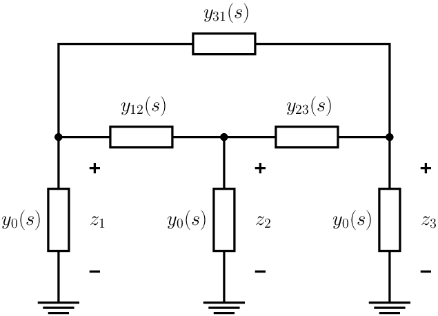
We now briefly discuss how far the range of condition (44) might extend. To this end we consider a generalization of the dynamics (37) employing the transfer function approach; see Fig. 8. In this general setting, each of identical oscillators22 2 Although we stick to the term oscillator, the general setting we consider here allows also systems that do not display oscillatory behavior, e.g., a single capacitor. is assumed to consist entirely of resistors, capacitors, and inductors, all LTI and passive, i.e., with positive resistance, capacitance, and inductance values. We denote by the admittance of an individual oscillator as seen from a given pair of terminals. One of those terminals is connected to the common ground and the other connects the oscillator to the rest of the network. In short, we represent each oscillator by an LTI passive one-port. As for coupling, the connection between a pair of oscillators is through also an LTI passive one-port (containing only resistors, capacitors, and inductors) with admittance . Note that . As before, we take and when there is no direct connection between the pair we have . The overall interconnection gives us , the -by- admittance matrix (4). The array of coupled oscillators, considered as a whole, we denote by . The network is said to synchronize if the node voltages (see Fig. 8) synchronize, i.e., for all and all initial conditions. (Note that here the initial condition, which determines the future evolution of the array, is the collection of all the initial capacitor voltages and initial inductor currents throughout the entire network.) In the sequel we will seek conditions guaranteeing the synchronization of .
Thanks to passivity we will be able to proceed in our analysis fairly rapidly. First, note that the eigenvalues that are observable from the node voltages have to be the (finitely many) roots of the characteristic polynomial where and the polynomials , are coprime. Since the network is passive those eigenvalues are confined to the closed left half-plane. Clearly, the ones with strictly negative real parts do not play any role in the steady state behavior of the network. This allows us to focus on the eigenvalues on the imaginary axis. Suppose now with is such an eigenvalue. Then (and only then) there exists a nonzero ( if ) and is a possible trajectory that can be traced by the node voltage vector . KCL imposes on this trajectory the constraint . In other words,
Therefore any steady state solution can be written as a sum of finitely many terms , where are distinct and are nonzero. Evidently, this steady state solution corresponds to a synchronized collection of node voltages if and only if for all . Note also that implies . Since , this means , i.e., . Hence we obtained:
Theorem 5
The network synchronizes if and only if
Also, for a synchronizing network, the steady state node voltages have the form with and satisfying .
Purists may rightfully contend that the subspace is not always well-defined because for certain frequencies either or some entries of may attain infinite magnitude. This however is only a minor mathematical obstacle, easy to circumvent by thinking in terms of the physical system that the model stands for. Consider the case . This means that the impedance is zero, i.e., the oscillators behave as short circuit at that particular frequency . As a result, all nodes are grounded, i.e., all the node voltages have to be zero, meaning . Consider now the other potentially ambiguous case, for certain pairs while . Note that implies that the nodes and are short-circuited, i.e., . To get rid of the infinite terms in the expression we can remove th and th rows from the matrix and inject the following two new rows: (i) the sum of the removed pair of rows and (ii) a row that imposes the equality . The cure can be repeated until all the infinite terms are gone. Let us demonstrate the procedure on an example network with nodes whose admittance matrix reads
Suppose that at some frequency the admittances and are infinite. This gives us the equalities and . Summing up the first three rows of lets us get rid of the terms and . Then we inject the extra rows and to represent the relation . Hence we can express as
with righthand side cleansed of the infinite terms. Incidentally, another relevant point we want to make has to do with the eigenvalues of . Since the roots of the polynomial are the eigenvalues of , we can use the procedure described above to define the finite eigenvalues of when some of its entries are infinite. For instance, for the previous example, the finite eigenvalues of , when and are infinite, are defined as the roots of the polynomial
Being thus able to single out the finite eigenvalues allows us to continue to use the notation , which will henceforth stand for the th smallest finite eigenvalue of with respect to the real part.
Consider now a network that does not synchronize. For this network Theorem 5 assures us that there exist a vector and a frequency satisfying and . Therefore is a (finite) eigenvalue of . Since the network is passive, all the eigenvalues of belong to the closed right half-plane, i.e., for all , whence . Also, again due to passivity, , whence . Consequently, . This implies, since , the matrix has at least two eigenvalues on the imaginary axis. This allows us to assert . To summarize:
Corollary 2
The network synchronizes if for all .
5 Conclusion
In this paper we studied the synchronization of identical (linear) pendulums coupled via dampers and springs. We first presented a necessary and sufficient condition for synchronization and then pointed out a sufficient set of conditions that may occasionally turn out to be easier to check than the former. Toward the end of the paper we applied the results obtained for pendulums to understanding better the collective behavior of coupled oscillators in LTI passive electrical networks. In particular, we established a relation between the second smallest eigenvalue of the node admittance matrix and the tendency of the individual systems to oscillate in unison.
References
- [1] R. Adato, A. Artar, S. Erramilli, and H. Altug. Engineered absorption enhancement and induced transparency in coupled molecular and plasmonic resonator systems. Nano Letters, 13:2584–2591, 2013.
- [2] V.I. Arnold. Mathematical Methods of Classical Mechanics (Second Edition). Springer, 1989.
- [3] C. Cai and S.E. Tuna. Synchronization of nonlinearly coupled harmonic oscillators. In Proc. of the American Control Conference, pages 1767–1771, 2010.
- [4] E. Fermi, J. Pasta, and S. Ulam. Studies on non linear problems. Los Alamos Document LA-1940, 1955.
- [5] T. Kapitaniak and J. Kurths (Eds). Synchronized pendula: From Huygens clocks to chimera states. European Physical Journal Special Topics, 223:609–612, 2014.
- [6] T. Kapitaniak, P. Kuzma, J. Wojewoda, K. Czolczynski, and Y. Maistrenko. Imperfect chimera states for coupled pendula. Scientific Reports, 4:6379, 2014.
- [7] L. Marcheggiani, R. Chacon, and S. Lenci. On the synchronization of chains of nonlinear pendula connected by linear springs. European Physical Journal Special Topics, 223:729–756, 2014.
- [8] W. Ren. Synchronization of coupled harmonic oscillators with local interaction. Automatica, 44:3195–3200, 2008.
- [9] H. Su, M.Z.Q. Chen, X. Wang, H. Wang, and N.V. Valeyev. Adaptive cluster synchronisation of coupled harmonic oscillators with multiple leaders. IET Control Theory and Applications, 7:765–772, 2013.
- [10] H. Su, X. Wang, and Z. Lin. Synchronization of coupled harmonic oscillators in a dynamic proximity network. Automatica, 45:2286–2291, 2009.
- [11] W. Sun, J. Lu, S. Chen, and X.Yu. Synchronisation of directed coupled harmonic oscillators with sampled-data. IET Control Theory and Applications, 8:937–947, 2014.
- [12] W. Sun, X. Yu, J. Lu, and S. Chen. Synchronization of coupled harmonic oscillators with random noises. Nonlinear Dynamics, 79:473–484, 2015.
- [13] H. Zhang and J. Zhou. Synchronization of sampled-data coupled harmonic oscillators with control inputs missing. Systems & Control Letters, 61:1277–1285, 2012.
- [14] J. Zhou, H. Zhang, L. Xiang, and Q. Wu. Synchronization of coupled harmonic oscillators with local instantaneous interaction. Automatica, 48:1715–1721, 2012.