Mathematical model of influence of friction on the vortex motion

Olga S. Rozanova Email: rozanova@mech.math.msu.su Corresponding author: Corresponding author Address: Department of Mechanics and Mathematrics, Moscow State University, Moscow 119992 Russia Jui-Ling Yu Address: Department of Financial and Computational Mathematics, Providence University, Taichung, 43301, Taiwan
and National Center of Theoretical Sciences at Taipei, Physics Division, National Taiwan University, Taipei 10617, Taiwan Chin-Kun Hu Address: Institute of Physics, Academia Sinica, Nankang, Taipei 11529, Taiwan
and National Center for Theoretical Sciences, National Tsing Hua University, Hsinchu 30013, Taiwan

August 24, 2026

Abstract

We study the influence of linear friction on the vortex motion in a non-viscous stratified compressible rotating media. Our method can be applied to describe the complex behavior of a tropical cyclone approaching land. In particular, we show that several features of the vortex in the atmosphere such as a significant track deflection, sudden decay and intensification, can be explained already by means of the simplest two dimensional barotropic model, which is a result of averaging over the height in the primitive equations of air motion in the atmosphere. Our theoretical considerations are in a good compliance with the experimental data. In contrast to other models, where first the additional physically reasonable simplifications are made, we deal with special solutions of the full system. Our method is able to explain the phenomenon of the cyclone attracting to the land and interaction of the cyclone with an island.

Keywords:

Mathematical model of atmosphere , Compressible fluid , Tropical cyclone , Surface friction , Topography

PACS

92.60Aa , 47.10ad , 92.60Pw

MSC

86A10

There exists a lot of theoretical, numerical, and experimental studies about the influence of land friction to the dynamics of tropical cyclones (e.g.[1] and references therein). However, they contain sometimes contradictory results. For example, some theoretical and numerical studies of the sensitivity of tropic cyclones to the friction in axisymmetric models indicated that the intensity decreases markedly as the drag coefficient increases [4], [5]. At the same time, in [6], [7], [8], the authors present a series of three-dimensional convection-permitting numerical experiments in which the intensification rate and intensity of the vortex increase with the surface drag coefficient up to a certain threshold value and then decrease. Further, the numerics made by MM5 (Fifth-Generation Penn State/NCAR Mesoscale Model) have shown that the phenomenon of attraction of the cyclone to the land does exist [9]. Moreover, many experimental works indicate that the circular air motion in cyclone transforms into a convergent air flow during the landfall [11].

Of course, the structure of a tropical cyclone is three-dimensional and the processes of the moisture and heat transfer play an important role in its formation. Nevertheless, we are going to show that several very complicated three-dimensional phenomena can be qualitatively explained by a relatively simple mechanical two-dimensional model where the topography is very crudely parameterized by allowing the surface friction coefficient to vary.

We deal with a special class of solutions of the full system, which is characterized by a linear profile of horizontal velocity. Under this condition we show that a smooth vortex in a material volume in three-dimensional stratified compressible non-barotropic flow and the simplest vortex in the two-dimensional barotropic model are governed by the same nonlinear system of ODEs.

We are going to show that the following phenomena related to the cyclone motion can be explained by a rather simple low parametric model analytically: (i) a drastic intensification of the cyclone and a deflection of its track during landfall; (ii) complex behavior of the cyclone during interacting with the land (attraction and rounding); (iii) formation of converging flow starting from circular motion inside the cyclone.

1 Full model of gas dynamics adapted for atmosphere

We consider the system of non-isentropic polytropic gas dynamics equations in a uniformly rotating reference frame for unknown functions $\rho\geq 0$ , $p\geq 0$ , $U=(U_{1},U_{2},U_{3})$ , $S$ (density, pressure, velocity and entropy), in the presence of a horizontal dry friction, namely

\rho(\partial_{t}U+(U,\nabla)U+le_{3}\times U+\mu U_{H}+ge_{3})=-\nabla p,

(1.1)

\partial_{t}\rho+{\rm div}(\rho U)=0,

(1.2)

\partial_{t}S+(U,\nabla S)=0.

(1.3)

The functions depend on time $t$ and on point $x\in{\mathbb{R}}^{3},$ $e_{3}=(0,0,1)$ is the ”upward” unit vector, $l$ is the Coriolis parameter, $\mu$ is the friction coefficient, $g$ is the acceleration due to gravity (points in $-e_{3}$ direction), $U_{H}=(U_{1},U_{2},0)$ , $\mu\geq 0$ is the friction coefficient. The state equation is

p=\rho^{\gamma}e^{S},

(1.4)

where $\gamma>1$ is the adiabatic exponent. This system is traditional, see e.g. [12], [13].

For our convenience taking into account (1.4) we write the equation (1.3) in terms of pressure:

\partial_{t}p+(U,\nabla p)+\gamma\,p\,{\rm div}U=0.

(1.5)

Let us consider classical solutions of (1.1), (1.2), (1.5). For $\mu=0$ , the system implies the conservation of mass ${\mathcal{M}}=\int\limits_{\Omega(t)}\rho\,dx$ , momentum ${\mathcal{P}}=\int\limits_{\Omega(t)}\rho U\,dx$ and energy

{\mathcal{E}}={\mathcal{E}}_{k}(t)+{\mathcal{E}}_{p}(t)=\int\limits_{\Omega(t)}\left(\frac{\rho|U|^{2}}{2}+\frac{1}{\gamma-1}p\right)\,dx,

inside a material volume $\Omega(t)$ , if we assume the hydrostatic balance

\partial_{x_{3}}p=-g\rho.

(1.6)

To prove these conservation laws we apply the formula for the derivative with respect to time of integral taken over a material volume [14], namely,

\frac{d}{dt}\int\limits_{\Omega(t)}f(t,x)dx=\int\limits_{\Omega(t)}\bigl(\partial_{t}f(t,x)+{\rm div}(f(t,x)\,U)\bigr)\,dx.

(1.7)

Let us introduce the following functionals:

G(t,x_{3})=\frac{1}{2}\int\limits_{\Omega_{H}(t)}\rho|{X_{1}}|^{2}\,d{x_{1}}d{x_{2}},\quad F_{i}(t,x_{3})=\int\limits_{\Omega_{H}(t)}({U,X}_{i})\rho\,d{x_{1}}d{x_{2}},

G_{x_{1}}(t,x_{3})=\frac{1}{2}\int\limits_{\Omega_{H}(t)}\rho x_{1}^{2}d{x_{1}}d{x_{2}},\quad G_{x_{2}}(t,x_{3})=\frac{1}{2}\int\limits_{\Omega_{H}(t)}\rho x_{2}^{2}d{x_{1}}d{x_{2}},

G_{x_{1}x_{2}}(t,x_{3})=\frac{1}{2}\int\limits_{\Omega_{H}(t)}\rho x_{1}x_{2}\,d{x_{1}}d{x_{2}},

where ${X}_{1}=(x_{1},x_{2}),\,{X}_{2}=(x_{2},-x_{1}),$ $\,i=1,2$ , $\Omega_{H}(t)$ is a section of $\Omega(t)$ at a fixed $x_{3}$ . We note that $G(t,x_{3})>0$ and $\Delta(t,x_{3})=G_{x_{1}}G_{x_{2}}-G_{x_{1}x_{2}}^{2}>0$ for nontrivial solutions to (1.1), (1.3), (1.5).

Let us consider $l=\rm const\geq 0$ and $\mu=\mu(x_{3})$ . Further, we assume $U_{3}=\Psi(t,x_{3})$ . The last assumption, (1.1), and (1.6) imply that $U_{3}(t,x_{3})$ satisfies the Hopf equation

\partial_{t}U_{3}+U_{3}\partial_{x_{3}}U_{3}=0,\quad x_{3}>0.

It is well known that if the initial data $U_{3}(0,x_{3})$ are not increasing, then the solution will lose the smoothness within a finite time. However, the natural conditions $U_{3}(t,0)=U_{3}(t,+\infty)=0$ imply that the initial datum $U_{3}(0,x_{3})$ is not increasing everywhere. Therefore the only possibility to consider a smooth solution for all $t>0$ is to set $U_{3}=0$ . This is the asymptotic of the solution containing shock waves as $t\to\infty$ on $(0,+\infty)$ for any initial data $U_{3}(0,x_{3})$ with the property $U_{3}(0,0)=U_{3}(0,+\infty)=0.$ Thus, the assumption $U_{3}=0$ satisfies this limit case.

Lemma 1.1

For the classical solutions of (1.1), (1.2), (1.5) with $U_{3}=0$ the following relations hold:

\partial_{t}G=F_{1},\quad\quad\partial_{t}F_{2}=lF_{1}-\mu F_{2},

\partial_{t}F_{1}=2(\gamma-1){E}_{p}+2{E}_{k}-lF_{2}-\mu F_{1},

\partial_{t}{E}=-2\mu{E}_{k},

where $E_{k}(t,x_{3})=\frac{1}{2}\int\limits_{\Omega_{H}(t)}{\rho|U_{H}|^{2}}\,d{x_{1}}d{x_{2}}\,$ , $\,E_{p}(t,x_{3})=\frac{1}{\gamma-1}\,\int\limits_{\Omega_{H}(t)}p\,d{x_{1}}d{x_{2}},$ $E=E_{k}+E_{p}$ .

Proof. To prove the identities it is enough to apply formula (1.7) with respect to the variables $x_{2}$ and $x_{2}$ . For example, taking into account (1.2), we get

\partial_{t}G=\frac{1}{2}\int\limits_{\Omega_{H}(t)}\partial_{t}\rho|X_{1}|^{2}\,dx_{1}dx_{2}=

\int\limits_{\Omega_{H}(t)}\Bigl(-\frac{1}{2}\,{\rm div}(\rho\,U)\,|{X}_{1}|^{2}+\frac{1}{2}\,{\rm div}\bigl(\rho\,U_{H}\,|X_{1}|^{2})\bigl)\Bigr)\,\,dx_{1}dx_{2}=

=\int\limits_{\Omega_{H}(t)}(X_{1},U)\,\rho\,dx_{1}dx_{2}=F_{1}.

The proof of other identities are analogous. $\square$

Let us assume a special structure of velocity inside $\Omega(t)$ . Namely, we set

U_{H}=Q_{H}{X_{1}},\quad Q_{H}=\left(\begin{array}[]{cc}a_{H}(t,x_{3})&b_{H}(t,x_{3})\\ c_{H}(t,x_{3})&d_{H}(t,x_{3})\end{array}\right),\quad U_{3}=0.

(1.8)

It is well known from experimental data that the profile of velocity near the center of atmospherical vortex like tropical cyclone is approximately linear [15]. Thus, we can consider the core of the cyclone as $\Omega(t)$ .

Lemma 1.2

For the velocity (1.8) we have

\partial_{t}G_{x_{1}}=2a_{H}G_{x_{1}}+2b_{H}G_{x_{1}x_{2}},\quad\partial_{t}G_{x_{2}}=2d_{H}G_{x_{2}}+2c_{H}G_{x_{1}x_{2}},

\partial_{t}G_{x_{1}x_{2}}^{\prime}=(a_{H}+d_{H})G_{x_{1}x_{2}}+b_{H}G_{x_{2}}+c_{H}G_{x_{1}},

\partial_{t}E_{p}=-(\gamma-1)(a_{H}+d_{H})E_{p},\quad\partial_{t}\Delta=2(a_{H}+d_{H})\Delta.

The potential energy $E_{p}$ is connected with $\Delta$ as

E_{p}(t,x_{3})=E_{p}(0,x_{3})\Delta^{(\gamma-1)/2}(0,x_{3})\Delta^{(-\gamma+1)/2}(t,x_{3}).

Proof. The proof is a direct computation with taking into account formula (1.7). The variable $x_{3}$ plays a role of parameter. $\square$

Let us introduce new functions

G_{1}={G_{x_{1}}}{\Delta^{-(\gamma+1)/2}},\quad G_{2}={G_{x_{2}}}{\Delta^{-(\gamma+1)/2}},\quad G_{3}={G_{x_{1}x_{2}}}{\Delta^{-(\gamma+1)/2}}.

Lemmas 1.1 and 1.2 imply that for the elements of the matrix $Q$ and $G_{1},\,G_{2},\,G_{3}$ can be obtained the following closed system of equations:

$\displaystyle\partial_{t}G_{1}$	$\displaystyle=$	$\displaystyle((1-\gamma)a_{H}-(1+\gamma)d_{H})G_{1}+2b_{H}G_{3},$
$\displaystyle\partial_{t}G_{2}$	$\displaystyle=$	$\displaystyle((1-\gamma)d_{H}-(1+\gamma)a_{H})G_{2}+2c_{H}G_{3},$
$\displaystyle\partial_{t}G_{3}$	$\displaystyle=$	$\displaystyle c_{H}G_{1}+b_{H}G_{2}-\gamma(a_{H}+d_{H})G_{3},$
$\displaystyle\partial_{t}a_{H}$	$\displaystyle=$	$\displaystyle-a_{H}^{2}-b_{H}c_{H}+lc_{H}-\mu a_{H}-\mathcal{K}G_{2},$	(1.9)
$\displaystyle\partial_{t}b_{H}$	$\displaystyle=$	$\displaystyle-b_{H}(a_{H}+d_{H})+ld_{H}-\mu b_{H}+\mathcal{K}G_{3},$
$\displaystyle\partial_{t}c_{H}$	$\displaystyle=$	$\displaystyle-c_{H}(a_{H}+d_{H})-la_{H}-\mu c_{H}+\mathcal{K}G_{3},$
$\displaystyle\partial_{t}d_{H}$	$\displaystyle=$	$\displaystyle-d_{H}^{2}-b_{H}c_{H}-lb_{H}-\mu d_{H}-\mathcal{K}G_{1},$

with $\mathcal{K}=\frac{\gamma-1}{2}E_{p}\Delta^{(\gamma-1)/2}|_{t=0}.$

Thus, (1.9) describes the behavior of full 3D system of dynamics of stratified atmosphere near the center of atmospherical vortex.For every fixed level $x_{3}=\bar{x}_{3}$ we have its own motion of air and the dynamics of the whole material volume is determined by $a(0,x_{3})$ , $b(0,x_{3}),$ $c(0,x_{3})$ , $d(0,x_{3})$ , $G_{1}(0,x_{3})$ , $G_{2}(0,x_{3})$ , $G_{3}(0,x_{3})$ .

Below we are going to show that the same system of ODE describes a behavior of the simplest possible solution of barotropic two-dimensional model of atmosphere.

2 Bidimensional models of the atmosphere

Since the horizontal scale in the atmospherical motion is much larger than the vertical scale, there exist many approaches to simplifying the model [16], [17]. Moreover, there is a possibility of averaging over the height to hide vertical processes and reduce the primitive system of equations to two space coordinates (see [18] for barotropic case and [19] for general case). Let us recall shortly the procedure of averaging. Let $\rho,\,U=(U_{1},U_{2},U_{3}),\,p,\,$ denote in the three-dimensional density, velocity and pressure. Namely, all these functions depend on $(t,x_{1},x_{2},x_{3}),$ $x_{3}\in\mathbb{R}_{+}$ . Let us introduce $\hat{\phi}$ and $\bar{f}$ to represent an average of $\phi$ and $f$ over the height, respectively. The averaged values are introduced as follows: $\displaystyle\hat{\phi}:=\int_{0}^{\infty}\phi\,dx_{3},\quad\bar{f}:=\frac{1}{\hat{\rho}}\int_{0}^{\infty}\rho f\,dx_{3}$ , where $\phi$ and $f$ are arbitrary functions, and denote $\varrho(t,{x_{1},x_{2}})=\hat{\rho},\,P(t,{x_{1},x_{2}})=\hat{p},\,{\bf U}(t,{x_{1},x_{2}})=(\bar{U}_{1},\bar{U}_{2}).$ Moreover, the usual adiabatic exponent, $\gamma$ , is related to the “two-dimensional” adiabatic exponent $\gamma_{H}$ as follows: $\gamma_{H}=\displaystyle\frac{2\gamma-1}{\gamma}<\gamma.$

The impenetrability conditions are included in the model. We require the vanishing of derivatives of the velocity on the Earth surface and a sufficiently rapid decay for all thermodynamic quantities as the vertical coordinate $x_{3}$ approaches to infinity. In other words, the impenetrability conditions assure the boundedness of the mass, energy, and momentum in the air column. They also provide the necessary conditions for the convergence of integrals.

If $l$ and $\mu$ are constant, the resulting two-dimensional system consists of three equations for density $\varrho(t,{\bf x}),$ velocity ${\bf U}(t,{\bf x})$ and pressure $P(t,{\bf x})$ , ${\bf x}\in{\mathbb{R}}^{2}$ :

\displaystyle\begin{split}\varrho(\partial_{t}{\bf U}+({\bf U}\cdot\nabla){\bf U}+{\mathcal{L}}{\bf U})+\nabla P&=0,\end{split}

(2.1)

\displaystyle\begin{split}\partial_{t}\varrho+{\rm div}(\varrho{\bf U})&=0,\end{split}

(2.2)

\displaystyle\begin{split}\partial_{t}P+({\bf U}\cdot\nabla P)+\gamma_{H}P\,{\rm div}{\bf U}&=0.\end{split}

(2.3)

Here $\mathcal{L}=lL+\mu I$ , $\quad L=\left(\begin{array}[]{cr}0&-1\\ 1&0\end{array}\right)$ , $I$ is the identity matrix, $\gamma_{H}\in(1,2)$ .

We used this model with $\mu=0$ in our previous papers [20], [21].

We can apply to (2.1)-(2.3) all considerations of Sec.1.

However, for us it will be convenient to restrict ourselves to the barotropic case, where $P={\mathcal{C}}\rho^{\gamma},\,{\mathcal{C}}={\rm const}$ . Thus, the system under consideration can be reduced to two equations (2.1), (2.2).

We introduce a new variable $\pi=P^{\frac{\gamma-1}{\gamma}}$ and get the system

	$\displaystyle\partial_{t}{\bf U}+({\bf U}\cdot\nabla){\bf U}+(l\,L\,+\mu\,I){\bf u}+c_{0}\,\nabla\pi=0,$		(2.4)
	$\displaystyle\partial_{t}\pi+(\nabla\pi\cdot{\bf U})+(\gamma-1)\,\pi\,{\rm div}\,{\bf U}\,=\,0,$		(2.4)

with $c_{0}=\frac{\gamma}{\gamma-1}{\mathcal{C}}^{\frac{1}{\gamma}}.$

2.1 A class of exact solutions

We consider a simple class of exact solutions which correspond to the first terms of expansion of $\pi$ at a critical point. Namely, we look for the solution in the form

{\bf U}(t,{\bf x})={Q}{\bf x},\qquad{Q}=\left(\begin{array}[]{cr}a(t)&b(t)\\ c(t)&d(t)\end{array}\right),

(2.5)

\pi(t,{\bf x})=A(t)x_{1}^{2}+B(t)x_{1}x_{2}+C(t)x_{2}^{2},

to get a closed ODE system for the components of the matrices $Q$ and $R=\left(\begin{array}[]{cr}A(t)&\frac{1}{2}B(t)\\ \frac{1}{2}B(t)&C(t),\end{array}\right)$ :

	$\displaystyle\dot{R}+RQ+Q^{T}R+(\gamma-1){\bf tr}QR=0,$		(2.6)
	$\displaystyle\dot{Q}+Q^{2}+lLQ+\mu Q+2c_{0}R=0.$		(2.6)

The system of matrix equations consists of 7 nonlinear ODEs and has a very complicated behavior. First of all, we discuss the behavior of the system in the frictionless case. In fact, an analogous class of solutions was considered in [23] in another context.

It can be readily checked that system (2.6), coincides formally with (1.9) at a fixed $x_{3}$ , where ${Q}=Q_{H}$ , $2c_{0}=\mathcal{K}$ , $A=G_{2}$ , $B=-2G_{3}$ , $C=G_{1}$ . Nevertheless, the nature of these systems is different and the components of solution of (2.6) are not a result of integration of corresponding components of solution of (1.9) with respect to $x_{3}$ . In particular, the constants $\gamma$ and $\gamma_{H}$ are different for these systems.

2.2 A friction-free vortex ( $\mu=0$ ), stability issue

2.2.1 Axisymmetric case [20]

It is easy to see that (2.6) has a closed submanifold of solutions having additional properties $a=d$ , $c=-b$ , $A=C$ , $B=0$ . These solutions corresponds to the axisymmetric motion. Note that it is the most interesting case related to the vortex in atmosphere. Here we get a system of 3 ODEs:

	$\displaystyle\dot{A}+2\gamma aA=0,$		(2.7)
	$\displaystyle\dot{a}+a^{2}-b^{2}+lb+2c_{0}A=0.$
	$\displaystyle\dot{b}+2ab-la=0,$

The functions $a,\,b,\,A>0$ correspond to one half of divergence, one half of vorticity and the fall of pressure in the center of vortex respectively. The only nontrivial equilibrium point that relates to a vortex motion is

a=0,\,b=-c=b^{*},\,A=A*=\frac{b^{*}(b^{*}-l)}{2c_{0}}.

The center of vortex corresponds to a domain of low pressure only if $A*>0$ (the motion is cyclonic). This implies $b^{*}<0$ or $b^{*}>l$ . Further, there exists one first integral

b=\dfrac{l}{2}+kA^{\frac{1}{\gamma}},

(2.8)

where $k$ is a constant [20]. Thus, (2.7) can be reduced to the following system:

\dot{A}=-2\gamma aA,\qquad\dot{a}=-a^{2}-\dfrac{l^{2}}{4}+k^{2}A^{\frac{2}{\gamma}}-2c_{0}A.

On the phase plane $\{(A,a),\,A>0\}$ , there always exists a unique equilibrium $(A^{*},a^{*})=(A_{0},0)$ , stable in the Lyapunov sense (a center), where $A_{0}$ is a positive root of equation

\dfrac{l^{2}}{4}+2c_{0}A=k^{2}A^{\frac{2}{\gamma}}.

2.2.2 General case

As follows from [24], the axisymmetric form of 2D vortex is stable with respect to asymmetric perturbations for the solution to the incompressible Euler equations. Indeed, the incompressibility condition implies $a(t)+d(t)=0$ and this reduces the full system (2.6) to (2.7). As we have shown in Sec.2.2.1, the equilibrium in this case is stable for any $b^{*}$ and $l$ .

Nevertheless, in the compressible case this property does not hold for arbitrary values of parameters.

Theorem 2.1

[22] If

b^{*}<\frac{1-\sqrt{2}}{2}\,l\quad\mbox{or}\quad b^{*}>\frac{1+\sqrt{2}}{2}\,l>l,

then the equilibrium of system (2.6) is unstable.

Proof. As one can readily check, the point

a=d=0,\,b=-c=b^{*},\,A=C=A*=\frac{b^{*}(b^{*}-l)}{2c_{0}},\,B=0

is the only equilibrium of the full system (2.6). It is the same point of equilibrium as in the axisymmetric case (2.7). Nevertheless, in the symmetric case this equilibrium is always stable in the Lyapunov sense, whereas in the general case the situation is different. Indeed, the eigenvalues of matrix corresponding to the linearization at the equilibrium point are the following:

\lambda_{1}=0,\quad\lambda_{2,3}=\pm\sqrt{-(2(2-\gamma)b^{*}(b^{*}-l)+l^{2})},

\lambda_{4,5,6,7}=\pm\sqrt{2}\,\sqrt{-l\left(b^{*}+\frac{l}{4}\right)\pm\sqrt{\left(b^{*}+\frac{l}{2}\right)^{2}\left(\frac{l^{2}}{4}+b^{*}l-(b^{*})^{2}\right)}}.

Since $(2-\gamma)b^{*}(b^{*}-l)+l^{2}>0$ for $\gamma\in(1,2)$ , then $\Re(\lambda_{2,3})=0$ . Eigenvalues $\lambda_{i},\,i=4,5,6,7$ have zero real part if and only if $b^{*}$ satisfies the following inequalities simultaneously: $l(b^{*}+\frac{l}{4})\geq 0,\quad\frac{l^{2}}{4}+b^{*}l-(b^{*})^{2}>0,$ $l^{2}\left(b^{*}+\frac{l}{4}\right)^{2}>\left(b^{*}+\frac{l}{2}\right)^{2}\left(\frac{l^{2}}{4}+b^{*}l-(b^{*})^{2}\right),$ that is $b^{*}\in\big[\frac{1-\sqrt{2}}{2}\,l,\,\frac{1+\sqrt{2}}{2}\,l\big]$ . For others values of $b^{*}$ the eigenvalues $\lambda_{4,5,6,7}=\pm\alpha\pm i\beta,\,\alpha\neq 0,\beta\neq 0$ , therefore there exist an eigenvalue with a positive real part. Thus, the Lyapunov theorem implies instability of the equilibrium for $b^{*}<\frac{1-\sqrt{2}}{2}\,l$ and $b^{*}>\frac{1+\sqrt{2}}{2}\,l>l.$ $\square$

Remark 2.1

We notice that the full system (2.6) has the first integral

b-c-l={\rm const}\,{\mathcal{D}}^{\frac{1}{2\gamma}},\quad{\mathcal{D}}=4AC-B^{2}.

This reduces (2.6) to the system of 6 equations. If $b^{*}\in\Sigma$ , $\Sigma=\left(\frac{1-\sqrt{2}}{2}l,0\right)\cup\left(l,\frac{1+\sqrt{2}}{2}l\right)$ , then the matrix, corresponding to the system, linearized at the equilibrium, has 3 pairs of pure imaginary complex conjugate roots $\lambda_{i},\,i=2,\dots,7$ (for the range of parameters under consideration the roots are simple). A study of stability in this case is extremely complicated and we will not dwell here (see [22]).

2.3 Influence of the friction on an axisymmetric vortex

The system of equations describing a vortex with a rotational symmetry is the following:

	$\displaystyle\dot{A}+2\gamma aA=0,$		(2.9)
	$\displaystyle\dot{a}+a^{2}-b^{2}+lb+2c_{0}A=-\mu a,$
	$\displaystyle\dot{b}+2ab-la=-\mu b,$

The solution to the equation has a complicated behavior, nevertheless it is possible to study it analytically to a certain extent.

Theorem 2.2

System (2.9) has two equilibriums $(a_{1}^{*},b_{1}^{*},A_{1}^{*})=(0,0,0)$ and $(a_{2}^{*},b_{2}^{*},A_{2}^{*})=(-\mu,l,0)$ , both are unstable.

Proof. Indeed, the matrix of the system linearized at the point $(A_{0},a_{0},b_{0})$ is

Q(A_{0},a_{0},b_{0})=\begin{pmatrix}-2\gamma a_{0}&-2\gamma A_{0}&0\\ -2c_{0}&-2a_{0}-\mu&2b_{0}-l\\ 0&-2b_{0}+l&-2a_{0}-\mu\end{pmatrix}.

The eigenvalues of $Q(0,-\mu,l)$ solve the equation

R(k)=(2\gamma\mu-k)((\mu-k)^{2}+l^{2})=0.

The polynomial has a positive root. This means instability of equilibrium $(-\mu,l,0).$ The eigenvalues of $Q(0,0,0)$ are $(0,-\mu\pm il)$ , therefore the linearized theory does not give an answer to the question about the stability or instability of zero equilibrium. However in the critical case we can use the theory of [25], Sec.4. Namely, we consider expansions into series $a(A)=a_{1}A+O(A^{2})$ and $b(A)=b_{1}A+O(A^{2})$ as $A\to 0$ . Then we substitute the expansions into (2.9) and get $a_{1}=-\frac{2\mu c_{0}}{\mu^{2}+l^{2}},$ $b_{1}=-\frac{2lc_{0}}{\mu^{2}+l^{2}}.$ Therefore $\dot{A}=\frac{4\gamma\mu c_{0}}{\mu^{2}+l^{2}}\,A^{2}+O(A^{2})$ . This implies instability of zero equilibrium. $\square$

Remark 2.2

Theorem 2.2 implies that the the zero equilibrium of the full system (2.6) is also unstable.

Theorem 2.3

The solutions to system (2.9) has no finite time blow up points at $t>0$ and the following inequalities hold:

\Lambda\leq\frac{c_{0}}{\gamma-1}A+k_{0}A^{\frac{1}{\gamma}}e^{-2\mu t},

(2.10)

A\leq K_{0}e^{\frac{2\mu\gamma}{2-\gamma}t},

(2.11)

where $\Lambda=\frac{a^{2}+b^{2}}{2}$ , $\delta_{0}$ , $K_{0}$ and $k_{0}$ are positive constants depending only on initial data.

Proof. First of all we note that the first equation and two latter equations of (2.9) imply

\dot{A}^{-1/\gamma}-2aA^{-1/\gamma}=0

(2.12)

and

\dot{\Lambda}+2a\Lambda+2c_{0}aA+2\mu\Lambda=0,

(2.13)

respectively. Equations (2.13) and (2.12) result

\frac{d}{dt}\,\left(\Lambda A^{-\frac{1}{\gamma}}-\frac{c_{0}}{\gamma-1}A^{\frac{\gamma-1}{\gamma}}\right)=-2\mu\Lambda A^{-\frac{1}{\gamma}}\leq 0.

(2.14)

From (2.14) we obtain (2.10).

Let us prove inequality (2.11). First of all we note that inequality (2.10) implies that there exists a constant $\bar{A},$ depending on initial data such that for $A>\bar{A}$ we have

\Lambda\leq k_{1}A

(2.15)

with a positive constant $k_{1}$ . Let us introduce a new variable $W=(b-\frac{l}{2})A^{-\frac{1}{\gamma}}e^{\mu t}.$ It is easy to check that

\frac{dW}{dt}=-\frac{l\mu}{2}A^{-\frac{1}{\gamma}}e^{\mu t}\leq 0.

(2.16)

As follows from (2.16), $W(t)\leq W(0).$ The second equation of (2.9) takes the form

a^{\prime}=-a^{2}-\mu a+W^{2}A^{2/\gamma}e^{-2\gamma\mu t}-2c_{0}A-\frac{l^{2}}{4}.

(2.17)

First, we consider the cases $l\mu=0,$ where $W(t)=W(0)$ , and $b(0)<\frac{l}{2}$ (or $W(0)<0$ ), for $l\mu\neq 0$ . Then (2.17) and (2.15) imply that for sufficiently large $A$ we have

a^{\prime}\geq W^{2}(0)A^{2/\gamma}e^{-2\gamma\mu t}-k_{2}A,\quad k_{2}>0.

(2.18)

Thus, if there exits an interval of $t$ such that the inequality

A^{\frac{2-\gamma}{\gamma}}>k_{3}e^{2\mu t},\quad k_{3}=k_{2}/W^{2}(0),

(2.19)

then for these $t$ the function $a(t)$ increases and, as follows from the first equation of (2.9), $A(t)$ decreases. Thus $A(t)$ increases if and only if inequality (2.11), opposite to (2.19), holds.

The last case is $l\mu\neq 0$ , $b(0)\geq\frac{l}{2}$ or $W(0)\geq 0$ . Due to (2.16) there are two possibilities: $W(t_{*})<0$ for some $t_{*}>0$ or $W(t)>W_{0}={\rm const}\geq 0$ for all $t>0$ . The first case can be reduced to the case $W(0)<0$ if we take $t_{*}$ as the initial moment of time. We note that $W(t)$ cannot be identically zero, this contradicts to the last equation of (2.9). If we assume $W_{0}>0$ , the second possibility implies inequality (2.18) with $W_{0}^{2}$ instead of $W^{2}(0)$ . Thus, estimate (2.11) follows from the same reasoning. Let us show that $W_{0}$ does not vanish and our assumption is correct. Indeed, from (2.15) we have

W\leq k_{4}A^{\frac{\gamma-2}{2\gamma}}e^{\mu t},\quad k_{4}={\rm const}>0,

(2.20)

for sufficiently large $A$ . Further, from (2.16) and (2.20) we obtain

\frac{dW}{dt}\geq-k_{5}W^{\frac{2}{2-\gamma}}e^{-\frac{\gamma\mu t}{2-\gamma}},\quad k_{5}={\rm const}>0.

(2.21)

We divide variables in (2.21) and integrate. After obvious estimates we get

W>\frac{W(0)}{(1+k_{5}(W(0))^{\frac{\gamma}{2-\gamma}})^{\frac{2-\gamma}{\gamma}}}:=W_{0}>0.

Thus, (2.11) is proved. $\square$

Remark 2.3

For $\mu=0$ inequalities (2.11) and (2.10) imply that the solution to system (2.7) is bounded for all $t>0$ by a constant depending on the initial data.

Remark 2.4

As follows from (2.16), the value of $W(t)$ is constant for $l\mu=0$ . From the conservation of $W$ for $\mu=0$ we get the integral (2.8).

Remark 2.5

Although systems (2.6) and (1.9) at a fixed $x_{3}$ are formally equivalent, we can obtain from (1.9) more information. Indeed, (2.6) is considered in the whole space ${\mathbb{R}}^{2}$ and it is not based on conservation laws. In contrast, (1.9) is considered in a moving volume, where the balance of energy $E^{\prime}(t)=-2\mu E_{k}(t)$ holds. Let us recall that the component $A(t)$ of solution of (2.6) corresponds to $G_{1}$ in the solution of (1.9). Since we deal with the axisymmetric case, $G_{1}=G_{2}=(G/2)^{-\gamma}$ . Let us note that if the velocity field has the form (2.5), $a=d,$ $c=-b$ , then $E_{k}=(a^{2}+b^{2})G\geq 0$ , $E_{p}=\delta_{1}G^{1-\gamma}\geq 0$ , $E_{k}+E_{p}\leq\delta_{2}$ , where $\delta_{1}$ and $\delta_{2}$ are positive constants, depending on initial data. This implies $G\geq\left({\delta_{1}}/{\delta_{2}}\right)^{\frac{1}{\gamma-1}}:=\delta_{3}>0$ . Thus, $G_{1}=(G/2)^{-\gamma}\leq(\delta_{3}/2)^{-\gamma}$ . In terms of system (2.6) this means that $A$ is bounded.

Figs.1 shows the behavior of functions $A(t)$ , related to the intensity for different periods of time (0-2 days, 2-2.3 days). The parameters are typical for geophysical vortex near its center. Namely, $c_{0}=0.1,\,\gamma=\frac{9}{7},\,l=7.3\cdot 10^{-5}\,s^{-1},\,b(0)=-5\cdot 10^{-6}\,s^{-1},\,A(0)=1.95\cdot 10^{-7}$ (solution to equation $b^{2}(0)-lb(0)-2c_{0}A(0)=0$ ). The parameter $\mu$ is $1\cdot 10^{-4}\,s^{-1}$ . The initial data correspond to a steady vortex for $\mu=0$ . One can see that in the presence of the land friction, the vortex first intensifies, after that a very fast oscillations begin. These oscillations can be interpreted as a destruction of the vortex. Moreover, the increasing amplitude of oscillations contradicts to boundedness of $A$ in a moving volume (Remark 2.5). Nevertheless, this contradicts only the smoothness of solution in the moving volume and implies the formation of frontal zone inside it.

Further, Figs.2 show the field of wind for a steady vortex in the non-frictional case and the respective field influenced by the constant surface friction for the period of intensification of vortex, as in the left Fig.1. We can see a formation of a convergent stream. Fig.2, right, is taken from [11] and presents the experimental evidence of the fact that the streamlines of the wind in a tropical cyclone form the focal point near the landfall. Thus, in the frame of the model it is possible to explain the formation of a convergent stream from an axisymmetric steady state.

Remark 2.6

The convergent inflow into cyclone is a well known feature of rotating boundary layers in general and can be explained be increasing of the Ekman pumping. Nevertheless this phenomenon can be explained within a two-dimensional non-viscous model.

Refer to caption — Figure 1: The intensification (left: 0 - 2 days) and destruction (right: 2 - 2.3 days) of the vortex, $A(t)$ (intensity), the time is in seconds.

3 Local and leading fields separation

Let us change the coordinate system of (2.4) in such a way that the origin of the new system ${\bf x}=(x_{1},x_{2})$ is located at a point ${\bf X}(t)=(X_{1}(t),X_{2}(t))$ . It is associated with the center of vortex (here and below we use the lowercase letters for $\bf x$ to denote the local coordinate system). Let ${\bf U}={\bf u}+{\bf V},$ where ${\bf V}(t)=(V_{1}(t),V_{2}(t))=(\dot{X}_{1}(t),\dot{X}_{2}(t))$ . Thus,

	$\displaystyle\partial_{t}{\bf u}+({\bf u}\cdot\nabla){\bf u}+$
	$\displaystyle\dot{\bf V}+(l\,L\,+\mu\,I)({\bf u}+{\bf V})+c_{0}\,\nabla\pi=0,$
	$\displaystyle\partial_{t}\pi+(\nabla\pi\cdot{\bf u})+(\gamma-1)\,\pi\,{\rm div}\,{\bf u}\,=\,0.$

Given a vector ${\bf V}$ , the trajectory of vortex can be found by integrating the system

\dot{X}_{1}(t)=V_{1}(t),\qquad\dot{X}_{2}(t)=V_{2}(t).

(3.1)

We assume that the pressure field can be separated into two parts

\pi=\pi_{0}(t,x_{1},x_{2})+\pi_{1}(t,x_{1},x_{2}).

The first field (we will call it local) is associated with the vortex, the second field can be considered as a leading one. In fact, the local field can be considered as a perturbation of the leading field due to the vortex. We impose a requirement

\nabla\pi_{0}|_{{\bf x}=0}=0.

Formally we can write

	$\displaystyle\big[\partial_{t}{\bf u}+({\bf u}\cdot\nabla){\bf u}+{\mathcal{L}}{\bf u}+c_{0}\,\nabla\pi_{0}\big]+$		(3.2)
	$\displaystyle\big[\dot{\bf V}+{\mathcal{L}}\,{\bf V}+c_{0}\,\nabla\pi_{1}\big]=0,$
	$\displaystyle\big[\partial_{t}\pi_{0}+(\nabla\pi_{0}\cdot{\bf u})+(\gamma-1)\,\pi_{0}\,{\rm div}\,{\bf u}\big]\,+$
	$\displaystyle\big[\partial_{t}\pi_{1}+(\nabla\pi_{1}\cdot{\bf u})+(\gamma-1)\,\pi_{1}\,{\rm div}\,{\bf u}\,\big]=\,0,$

Let us denote

\displaystyle q=c_{0}\left[\nabla\pi_{1}(t,{\bf x})-\nabla\pi_{1}(t,{\bf x})\Big|_{{\bf x}=0}\right].

(3.3)

If we solve separately the system for the local field

	$\displaystyle\partial_{t}{\bf u}+({\bf u}\cdot\nabla){\bf u}+{\mathcal{L}}\,{\bf u}+c_{0}\,\nabla\pi_{0}+q=0,$
	$\displaystyle\partial_{t}\pi_{0}+(\nabla\pi_{0}\cdot{\bf u})+(\gamma-1)\,\pi_{0}\,{\rm div}\,{\bf u}=\,0,$

we get a linear equation for $\pi_{1}$ :

\displaystyle\partial_{t}\pi_{1}+(\nabla\pi_{1}\cdot{\bf u})+\pi_{1}{\rm div}{\bf u}=0,

(3.4)

which can be solved for any initial condition $\pi_{1}(0,{\bf x})$ .

Further, from (3.2) we obtain

\displaystyle\dot{\bf V}(t)+{\mathcal{L}}{\bf V}(t)+c_{0}\nabla\pi_{1}(t,{\bf x})\Big|_{{\bf x}=0}=0,

(3.5)

then (3.5) and (3.3) result

\displaystyle\ddot{\bf X}(t)+{\mathcal{L}}\dot{\bf X}(t)+c_{0}\nabla\pi_{1}(t,{\bf x})\Big|_{{\bf x}=0}=0.

If $q=0$ , then we obtain a complete separation of two processes and the local field does not depend of the leading field. It is easy to see that $q=0$ if and only if $\pi_{1}$ is linear with respect to the space variables. If $q\neq 0$ , however it is in some sense small, we can talk about an approximate separation of processes; $|q|$ plays a role of measure of separability of the local and leading processes.

4 Influence of friction on the trajectory of vortex

If the couple $({\bf u},\pi_{0})$ is found, then the position of the vortex can be determined from linear equations (3.4) and (3.3). Let $({\bf u},\pi_{0})$ be the exact solution considered in Sec.2.1. As follows from (3.4), if

\pi_{1}(0,x_{1},x_{2})=M(0)x_{1}+N(0)x_{2}+K(0),

then the initial field $\pi_{1}$ is linear with respect to the space variables, that is

\pi_{1}(t,x_{1},x_{2})=M(t)x_{1}+N(t)x_{2}+K(t).

Thus, we obtain the zero discrepancy term $q$ (i.e. the complete separation of local and leading fields). The coefficients $M(t),$ $N(t)$ and $K(t)$ can be found from the ODE system

	$\displaystyle\dot{M}+(2\gamma-1)aM-bN=0,$		(4.1)
	$\displaystyle\dot{N}+(2\gamma-1)aN+bM=0,$
	$\displaystyle\dot{K}+2(\gamma-1){\bf tr}QK=0.$

To obtain the trajectory of the center of vortex $(X_{1}(t),X_{2}(t))$ , we have to solve the system (3.5), which can be reduced to

	$\displaystyle\dot{V}_{1}-lV_{2}+\mu V_{1}+c_{0}M=0,$		(4.2)
	$\displaystyle\dot{V}_{2}+lV_{1}+\mu V_{1}+c_{0}N=0.$		(4.2)

Then the trajectory can be found from (3.1). The coefficients $M(t)$ and $N(t)$ can be considered as a measure of intensity of the leading field. It is natural to assume that they are so small that the local field can be discerned in the leading field (see the numerical examples from [21]). The function $K(t)$ does not influence the trajectory.

4.0.1 Constant coefficient of surface friction

As we have shown, the friction basically causes the intensification of vortex. At the same time, the trajectory of vortex changes according to the leading field and initial velocity. It can shrink or amplify, formation of loops is a typical behavior. Fig.3 shows the position of vortex, computed for the parameters corresponding to a tropical cyclone within two days for $\mu=0$ and $\mu=2\cdot 10^{-5}{\rm s}^{-1}$ respectively. The Coriolis parameter $l=7.3\times 10^{-5}\,{\rm s}^{-1},$ that corresponds to the latitude $30^{\circ}\,$ approximately, $c_{0}=0.1$ (appropriate dimension), $\gamma=\frac{9}{7}$ (recall that in the procedure of averaging over the height, the value of heat ratio for air changes). Initial data are the same for the both cases, namely, $V_{1}(0)=V_{2}(0)=1$ m/s, $M(0)=N(0)=10^{-3}$ (appropriate dimension), $b^{*}=-10^{-6}{\rm s}^{-1}$ , initial condition corresponds to equilibrium for $\mu=0.$

4.0.2 Influence of a land: interaction of vortex with the ”island”

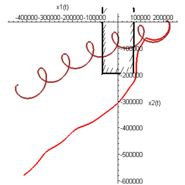
The most intriguing phenomenon is the interaction of the cyclone with the land. There are a lot of experimental and numerical evidences showing that the cyclone ”feels” the land; it can be attracted to the shore, but sometimes it ”avoids” the shore, on the contrary [10], [2], [3]. Now we are going to show that the approximation of trajectory made by the ODE system (2.9),(4.1),(4.2), (3.1) can reproduce this complicated behavior. The coefficient of surface friction $\mu$ in this experiments is a function of space variables $X_{1},X_{2}$ . It changes from zero (sea surface) to some constant value $\mu_{0}$ (”island”). Let $\mu(X_{1},X_{2})=\omega(X_{1},X_{2})\mu_{0}$ ,

\displaystyle\omega(X_{1},X_{2})=\prod_{k=1}^{2}\left(\arctan\left(\frac{X_{k}(t)+\bar{x}_{k}}{\sigma}\right)-\arctan\left(\frac{X_{k}(t)-\bar{x}_{k}}{\sigma}\right)\right),

where $\sigma$ is a very small constant. The square $[-\bar{x}_{1},\bar{x}_{1}]\times[-\bar{x}_{2},\bar{x}_{2}]$ corresponds to the island, the motion begins over the sea.

Fig.4 shows that the attraction to the lands increases with the roughness of the land. Fig.5 shows the difference of divergence and intensity for different roughness of the island. Fig.6 shows that for some initial conditions, the cyclone can avoid the island.

5 Conclusion

To study different properties of vortices in a compressible medium (e.g. atmosphere), we analyze a special class of smooth motions characterized by a linear profile of the horizontal velocity. It is well known that the velocity has this property near the center of vortex (e.g.[15]). We consider two models: the primitive 3D model of atmosphere and 2D model obtained from it by the standard averaging procedure.

In the latter model we make additional assumption about barotropicity of the process to obtain a system having an exact solution in the form of the first terms of the Taylor expansion in the center of vortex. Thus, we get a system of two equations. We could obtain the same result by assuming that the process is isochoric, i.e. the pressure is proportional to the temperature. We study the influence of the linear friction on the behavior of vortex.

We show that in the case of atmosphere, where the vertical motion satisfies the hydrostatic balance and the horizontal and vertical motion are somewhat separated, the vortex behavior can be described by the same system of ODEs as the vortex in the 2D barotropic model. The vertical coordinate can be considered as a parameter.

First of all, we consider a steady axisymmeric vortex in the friction-free case and show that in contrast to the incompressible case, there exist some parameters such that the vortex is unstable with respect to small perturbations of initial symmetry in the class of solution with a linear profile of velocity.

Further, we prove that the vortex always loses the stability when the surface friction coefficient is constant. We note that the flutter instability (a blowing-up vibrational motion) can be induced by dry friction in mechanical systems which would be stable without frictional forces (e.g.[26]).

Finally, we study an axisymmetric vortex in the case of constant surface friction both analytically and numerically and show that the complicated features of the vortex (e.g. a sudden decay and further intensification) can be explained by our model. Moreover, we have shown that the phenomenon of interaction of the tropical typhoon with land can be quite realistically explained by a relatively simple ODE system, where the effect of topography is modeled by variable surface friction coefficient.

The aim of our study is to show that many interesting effect of the atmospherical vortex motion can be qualitatively explained already by a very simple mechanical model. Of course, we do not pretend to claim that the trajectories of real tropical cyclones can be entirely explained by this model. There are at least three reasons for this. First of all, the real atmospheric vortex is localized and has structure (3.2) only in a vicinity of its center. The exact solution with linear profile of velocity gives the exact separation of local and leading fields only if the leading field is also linear with respect to the space variables. In this case the discrepancy $q=0$ (see (3.3)) and the position of the center of vortex can be computed from the nonlinear system of ODEs (2.9),(4.1),(4.2), (3.1) exactly. If the velocity and pressure have a more realistic localized structure, then the discrepancy $q\neq 0$ . Nevertheless, as follows from (3.4), $q$ remains small until the divergence of the velocity of the local field is small. As we have shown in [21], for the case $\mu=0$ , the difference between position of the center obtained from the ODE system and the position of the localized vortex obtained from direct numerical computations can be very small within several days. The second reason is that for big velocities the drag friction coefficient $\mu$ depends on velocity itself (thus, the surface stress parametrization should be quadratic). Nevertheless, as one can easily see from (1.1), the quadratic drag friction together with the geostrophic condition $\rho lL{U_{H}}+\nabla_{H}p=0$ ( $\nabla_{H}$ stands for the horizontal gradient) lead to a fast singularity formation for any realistic profile of velocity. Therefore, this kind of friction worsens the smoothness of the solution significantly. The third reason also relates to our assumption about the smoothness of solution. Indeed, as we have shown in Remark 2.5, the fact of the envelope of oscillations growing with time contradicts to the conservation of energy for the moving volume. This contradiction can be removed if we assume a formation of shock wave within the volume. Therefore, we can say that the ”theoretical” trajectory of vortex is close to a real one only for some period of time depending on initial data. The computations made for realistic parameters suggest that this interval is less than one day. Therefore the rising oscillations that one can see in the solution of the nonlinear system of ODE cannot develop.

All these questions about correspondence of theoretical and real vortex can be solved only numerically. The influence of different kinds of friction on the trajectory of a localized vortex and comparisons with the trajectory computed from (2.9),(4.1),(4.2), (3.1) are the issues of our future researches.

ACKNOWLEDGMENTS

OSR thanks Dr.A.Akhmetzhanov and M.Turzynsky for a valuable discussion.

JLY was supported by the grant of NSC 102-2115-M-126-003 and thanks Academia Sinica for supporting the summer visit. OSR was supported by Mathematics Research Promotion Center, MOST of Taiwan and RFBR Project Nr.12-01-00308.

References

[1] Wong, M.L.M., Chan, J.C.L. Tropical cyclone motion in response to land surface friction. J. Atm. Sci., 2006, 63, 1324–1337.
[2] Tang, C.K., Chan, J.C.L. Idealized simulations of the effect of Taiwan topography on the tracks of tropical cyclones with different sizes. Q. J. R. Meteorol. Soc. 5 NOV 2015, DOI: 10.1002/qj.2681
[3] Tang, C.K., Chan, J.C.L. Idealized simulations of the effect of Taiwan and Philippines topographies on tropical cyclone tracks. Q. J. R. Meteorol. Soc. 2014, 140(682 Part A), 15781589.
[4] Emanuel, K.A. Sensitivity of tropical cyclones to surface exchange coefficients and a revised steadystate model incorporating eye dynamics. J. Atmos. Sci., 1995, 52, 3969–3976.
[5] Craig, G.C., Gray, S.L. CISK or WISHE as a mechanism for tropical cyclone intensification. J. Atmos. Sci. 1996, 53, 3528–3540.
[6] Montgomery, M.T., Smith, R.K., Nguyen, S.V. Sensitivity of tropical-cyclonemodels to the surface drag coefficient, Q. J. R. Meteorol. Soc., 2010, 136, 1945–1953.
[7] Smit, R.K., Montgomery, M.T., Thomsen, G.L. Sensitivity of tropical-cyclone models to the surface drag coefficient in different boundary-layer schemes, Q.J.R. Meteorol. Soc., 2014, 140, 792–804.
[8] Luo, G., Gao, Y. Influence of mesoscale topography on vortex intensity. Progress in Natural Science, 2008, 18, 71–78.
[9] Kuo, H.C., Williams, R.T., Chen, J.H., Chen, Y. L. Topographic effects on barotropic vortex motion: No mean flow, J. Atmos. Sci., 2001, 58, 1310–1327.
[10] Yuan J.-N., Huang Y.Y., Liu C.-X., Wan Q.-L. A simulation study of the influence of land friction on landfall tropical cyclone track and intensity, J. Trop. Meteor. 2008,14, 53–56.
[11] Powel, M.D. The transition of the hurricane Frederic boundary-Layer wind field from the open gulf of Mexico to landfall. Mon. Wea. Rev., 1982, 110, 1912–1932.
[12] Landau, L.D., Lifshits, E.M. Fluid mechanics. 2nd ed., Volume 6 of Course of Theoretical Physics. Oxford etc.: Pergamon Press, 1987.
[13] Pedlosky, J. Geophysical fluid dynamics. NY:Springer-Verlag, 1979.
[14] Chorin, A.J., Marsden, J.E. A Mathematical Introduction to Fluid Mechanics, Springer: New York, 2000.
[15] Sheets, R.C. On the structure of hurricanes as revealed by research aircraft data, In Intense atmospheric vortices. Proceedings of the Joint Simposium (IUTAM/IUGC) held at Reading (United Kingdom) July 14-17, 1981, edited by L.Begtsson and J.Lighthill, pp.33–49, 1982 (Berlin-Heidelberg-New York, Springer-Verlag).
[16] Durran, D.R., Arakawa A. Generalizing the Boussinesq approximation to stratified compressible flow, Comptes Rendus Mecanique, 335 (2007) 655-664.
[17] White, A.A., Hoskins, B.J., Roulstone, I., Staniforth, A. Consistent approximate models of the global atmosphere: shallow, deep, hydrostatic, quasihydrostatic and non-hydrostatic. Q. J. R. Meteorol. Soc., 131 (2005), 2081-2107.
[18] Obukhov, A.M. On the geostrophical wind Izv.Acad.Nauk (Izvestiya of Academie of Science of URSS), Ser. Geography and Geophysics, 1949, XIII, 281–306.
[19] Alishaev, D.M. On dynamics of two-dimensional baroclinic atmosphere Izv.Acad.Nauk, Fiz.Atmos.Oceana, 1980, 16, N 2, 99–107.
[20] Rozanova, O.S, Yu, J.-L., Hu, C.-K. Typhoon eye trajectory based on a mathematical model: Comparing with observational data. Nonlinear Analysis: Real World Applications, 2010, 11, 1847–1861.
[21] Rozanova, O.S, Yu, J.-L., Hu, C.-K. On the position of vortex in a two-dimensional model of atmosphere. Nonlinear Analysis: Real World Applications, 2012, 13, 1941–1954.
[22] Rozanova, O.S, Yu, J.-L., Turzynsky M.K., Hu, C.-K. Nonlinear stability of two-dimensional axisymmetric vortices in compressible inviscid medium in a rotating reference frame. ArXiv e-prints: 1511.07039, 2015.
[23] Ball, F.K. An exact theory of simple finite shallow water oscillations on a rotatirig earth. 1st Australasian conference on hydraulics and fluid mechanics: proceedings (ed. R. Silvester). MacMillan, 1964, 293, 293–305.
[24] Schecter, D.A., Dubin, D.H.E., Cass, A.C., Driscoll, C.F., Lansky, I.M., O’Neil, T.M. Inviscid damping of asymmetries on a two-dimensional vortex. Phys. Fluids, 2000, 12, 2397.
[25] Malkin, I.G. Theory of stability of motion. Translation series ACC-TR-3352: Physics and mathematics, US Atomic Energy Commission, 1958.
[26] Bigoni, D. Nonlinear solid mechanics bifurcation theory and material instability. Cambridge University Press, 2012.