Islands of stability and recurrence times in AdS
Abstract
We study the stability of anti–de Sitter (AdS) spacetime to spherically symmetric perturbations of a real scalar field in general relativity. Further, we work within the context of the “two time framework” (TTF) approximation, which describes the leading nonlinear effects for small amplitude perturbations, and is therefore suitable for studying the weakly turbulent instability of AdS—including both collapsing and non-collapsing solutions. We have previously identified a class of quasi-periodic (QP) solutions to the TTF equations, and in this work we analyze their stability. We show that there exist several families of QP solutions that are stable to linear order, and we argue that these solutions represent islands of stability in TTF. We extract the eigenmodes of small oscillations about QP solutions, and we use them to predict approximate recurrence times for generic non-collapsing initial data in the full (non-TTF) system. Alternatively, when sufficient energy is driven to high-frequency modes, as occurs for initial data far from a QP solution, the TTF description breaks down as an approximation to the full system. Depending on the higher order dynamics of the full system, this often signals an imminent collapse to a black hole.
I Introduction
Of the maximally symmetric solutions of the Einstein equation, nonlinear stability in general relativity has been proven for both Minkowski [1] and de Sitter [2] spacetimes. In contrast, the question of stability of anti–de Sitter (AdS) remains formally open. A key differentiator of AdS as compared to its counterparts is that with non-dissipating boundary conditions at infinity, perturbations cannot decay and energy is conserved [3]. Based on knowledge of nonlinear wave propagation in the absence of dissipation, AdS has been conjectured to be unstable [4, 5] (see also [6]). This expectation has been corroborated by numerical simulations—supported by perturbative arguments—which showed that certain initial configurations evolve to black holes, no matter how small the initial deviation from AdS was taken [7]. This work showed, further, that the eventual gravitational collapse resulted from a turbulent cascade of energy to high-frequency modes of AdS, mediated by resonant interactions.
Instability of AdS would have implications for a number of fields, ranging from potential gravitational instabilities in other low-dissipation or confining geometries, to thermalization of conformal field theories (CFTs). In the context of AdS/CFT (within the regime where general relativity holds in the bulk), the formation and subsequent evaporation of a black hole in AdS is believed to be dual to the process of CFT thermalization. The more recent discovery of initial configurations in the bulk that appear to avoid black hole formation [8] was, therefore, somewhat surprising, as that would indicate non-thermalizing CFT configurations. This finding led to the identification of several “islands of stability” in AdS [9, 10, 11].
Significant progress towards an analytic understanding of the dynamics was achieved with the introduction of a powerful perturbative framework—the two time framework (TTF)—for analyzing small perturbations of AdS in terms of coupled nonlinear oscillators [12] (see also [13]). This framework efficiently captures the resonant energy-exchange interactions between normal modes, while effectively “integrating out” high-frequency oscillations. TTF led to the discovery of a pair of quantities—the energy and particle number —that are conserved at the leading nonlinear level [14, 15]. These quantities play key roles in understanding long-term dynamical behaviors, including dual (direct and inverse) turbulent cascades and non-equipartition of energy [15].
The main purpose of this paper is to establish a large new class of islands of stability within the TTF approximation. The central stable equilibria—quasi-periodic (QP) solutions [12, 15]—form discrete families, each family itself parametrized by and . In this work we (i) construct the families of equilibrium solutions, (ii) perform a linear stability analysis within TTF showing stability, and (iii) use the results to understand the long-term behavior of both collapsing and non-collapsing initial configurations. In particular, the stability analysis gives rise to a perturbation spectrum that agrees with and explains “recurrences”—long-term nearly-periodic approaches of the configuration to the initial state, first observed in the Fermi-Pasta-Ulam (FPU) system of coupled oscillators [16]—which were observed numerically in the full system. Dependence of the families of QP solutions on the two continuous parameters and extends previously known one-parameter families (time-periodic solutions [10]) and provides a clear connection between conserved quantities and stable islands.
I.1 Background
Following [7], we restrict analysis to the spherically symmetric case and four spacetime dimensions. As a proxy for gravitational degrees of freedom, we take as our model a real massless scalar field coupled to general relativity. Ignoring gravity, the scalar field is characterized by normal modes with spatial wavefunctions
| (1) |
and frequencies ().
Since the frequency spectrum is commensurate, nonlinear gravitational interactions are resonant, and those interactions cause energy to be readily transferred among the modes11 1 The frequency spectrum is also resonant with a massive scalar, for other spacetime dimensions, and in the absence of spherical symmetry.. Numerical simulations have shown that for certain initial data, energy is transferred from low- to high- modes—a direct turbulent cascade [7]. This cascade concentrates the energy—the high- modes are more highly peaked in position space—and eventually leads to black hole formation. The cascade behavior persists self-similarly as the amplitude of the initial scalar field is decreased, with the time to collapse scaling as (see, e.g., Fig. 2 of [7]).
In contrast, other initial data seem to avoid collapse22 2 Simulations are of finite duration, and the limit cannot be obtained numerically, so collapse-avoidance is a conjecture. as . In addition to direct cascades, these solutions feature inverse turbulent cascades, which transfer energy to low- modes [17, 12]. Collapse is avoided if the inverse cascades sufficiently hinder the flow of energy to high- modes.
A key observation is that energy cascades and normal mode oscillations are governed by independent time scales. As , nonlinear interactions become weaker—the stress-energy tensor , and gravitational self-interactions of scale as —so the energy transfer time scale is proportional to . Meanwhile, normal mode oscillations proceed independently of . This separation of time scales means we can use multiscale analysis methods to study the slow mode-mode interactions independently of the fast normal mode oscillations in the limit [12].
We define the “slow time” . Over short time scales the scalar field is well-approximated as a sum over normal modes. Thus, we take as ansatz , with
| (2) |
At lowest nonlinear order, we showed that gravitational self-interactions of are taken into account provided the coefficients satisfy the coupled ordinary differential equations [12],
| (3) |
known as the two time framework (TTF) equations. The TTF equations were also derived using renormalization group perturbation methods to re-sum secularly growing terms that arise in ordinary perturbation theory [13]. Notice that the TTF equations possess the same scaling symmetry, seen in the full (non-TTF) system in the limit .
The numerical coefficients appearing in (3) arise from overlap integrals involving the , and they vanish unless . This fact, together with the specific form of the equations (3) (i.e., the lack of terms such as , etc.), arises because the only resonances that are present in the system are those such that [13]
| (4) |
This property is related to a hidden symmetry in AdS [18]. For further discussion on the absence of certain resonance channels, see [19].
Within their regime of validity, the TTF equations yield approximate solutions much more economically than full numerical relativity simulations [12]. Indeed, a significant speedup is gained by not modeling the rapid normal-mode oscillations. Moreover, the TTF approximation improves as —a limit that is especially hard to reach in numerical relativity. Nevertheless, in the same way that finite difference methods employ a discrete spatial grid, the set of TTF equations (3) must in practice be truncated at finite (similar to pseudo-spectral methods). Previously, we computed (by performing explicit integrations on a mode-by-mode basis) the coefficients up to [12]. We now have closed form expressions for the coefficients (see App. A) that enable us to work to much larger . We typically set in this paper, which in many cases provides an excellent approximation. In particular, the recurrence dynamics of non-collapsing solutions are well-captured.
While useful as a calculational tool, the main power of TTF is analytic33 3 See also [20] for another recent illustration of the power of this approach within general relativity.. Indeed, in [14, 15] it was uncovered that the TTF equations conserve a total of three quantities: The total energy and particle number,
| (5) | |||||
| (6) |
as well as the Hamiltonian44 4 As described in detail in [14], the system (3) in the “origin-time” spacetime gauge of [7, 12, 13] is not a Hamiltonian system itself. However, in the “boundary-time” gauge of [8, 17] the system is Hamiltonian with Hamiltonian . Both gauges possess the same conserved quantities, so in this paper we shall refer to as the “Hamiltonian”, despite working in origin-time gauge (for comparison with prior numerical simulations). Note also that the equivalent expression in [15] did not include the second term in .,
| (7) |
where are additional constants. Conservation laws of and are associated with two symmetries,
| (8) | |||||
| (9) |
respectively, for constant; conservation of is associated with time-translation symmetry [14]. (The symmetries and associated conservation laws were first uncovered for the TTF equations that describe a non-gravitating scalar field in AdS4, with quartic self-interaction [21].) Simultaneous conservation of and implies that direct and inverse turbulent cascades must occur together, and that energy equipartition is in general not possible [15].
Finally, we showed in [12] that the TTF equations give rise to equilibrium solutions, which are QP. That is, each mode amplitude,
| (10) |
with . Simulations in TTF and full numerical relativity both provided evidence for stability of these QP solutions. The case was then made in [15] that general non-collapsing solutions can be treated as perturbations about associated QP solutions—in other words, QP solutions with the same and . As an example application, we studied two-mode initial data, which exhibits FPU-like [16] recurrences over long time scales. We showed, by interpolating initial data between two-mode and associated QP, that the recurrence times were only marginally affected. We therefore concluded that a proper stability analysis might predict these times, and QP solutions might provide anchor points for the “islands of stability” in AdS.
I.2 Summary
In this paper we present a comprehensive analysis of QP solutions and their relation to AdS (in)stability. After presenting the algebraic equations governing QP solutions in Sec. II, we show that they extremize for first order variations holding and fixed. We then numerically map out the space of solutions to the QP equations. This space can be divided into a number of families of solutions, each one depending on two continuous parameters, and . Because of the scaling symmetry of the TTF equations, these families are scale-invariant, so it is often useful to exchange and for an overall scale, and the ratio —which we identify with the “temperature.”
In Sec. III we perform a linear stability analysis of QP solutions within TTF. We uncover two 2-dimensional subspaces of special perturbations: the first corresponds to a pair of generators of the symmetries (8) and (9) of TTF; the second represents infinitesimal perturbations to nearby QP solutions with different and . (We make use of these special perturbations to generate the continuous families of QP solutions parametrized by and in Sec. II.) The remaining perturbations preserve and , and may be decomposed into eigenmodes describing small oscillations. The corresponding eigenvalues determine stability. We present a numerical method to perform this stability analysis given any particular background QP solution.
After presenting the framework for analyzing stability, we apply it to the families of QP solutions identified in Sec. II. We argue, by explicitly checking a large number of QP solutions, that the “physical” families—those that do not depend strongly on the mode cutoff in the limit —are all stable. By contrast, QP solutions that are not members of these families can have unstable modes.
In Sec IV we apply the results of the stability analysis to understand long-term evolutions. Since and are conserved, motion in phase space is constrained to constant- hypersurfaces. Each surface intersects a given stable QP family at most once, resulting in a discrete collection of QP solutions. If initial data lies within the -trough around one of these QP solutions with the same , then we associate it to that QP solution. Under evolution the solution is then confined to oscillate about its associated QP solution. We illustrate, through several examples, how nonlinear evolutions of initial data within TTF inherit many of the properties uncovered by the linear stability analysis. In particular, the linear stability analysis explains nonlinear recurrences as oscillations about QP solutions, and the eigenmodes (and combinations thereof) predict the recurrence times. Thus, we obtain approximate recurrence times without performing any time integrations. This approach to understanding recurrences is a generalization (to two conserved quantities) of the -breather approach to understanding FPU recurrences [22, 23].
For evolutions that remain close to stable QP solutions, the energy spectra remain close to the exponential energy spectra of the QP solutions. In contrast, solutions that are not close to QP solutions tend to approach power laws in TTF, consistent with earlier studies [24]. A power law spectrum contains far more energy at high-, and when translated to a description involving spacetime fields at finite , the energy is far more concentrated at the origin of AdS; in fact, it fails to even converge in . When deviations from AdS become large, TTF no longer applies, and higher-order dynamics take over. It is often the case that the higher order dynamics rapidly drive collapse once they take hold [7]; the role of TTF is to indicate whether this regime is reached.
It is important to keep track of the various levels of levels of approximation used in this work, so we summarize them here. First, the TTF equations are taken as an approximation to the full system, valid in the limit55 5 For an interesting discussion of when solutions of the approximated system might correspond to solutions of the full system, see [25]. . Secondly, we truncate the TTF system at a finite number of modes. Finally, we perform a linear stability analysis of QP solutions within the truncated TTF system. Throughout this work we will address the validity of the various approximations.
II Quasi-periodic solutions
There is already strong evidence that there are stable equilibrium solutions—islands of stability—in AdS, namely the time-periodic solutions [7, 10]. These solutions are nonlinear generalizations of individual normal modes, with the effect of gravity being to shift the frequency. Such solutions are moreover realized as solutions to the TTF system (3) of the form
| (11) |
for some fixed mode number . (The analysis of [10], however, is accurate to higher order in .) For a given there exists a 1-parameter family of solutions, parametrized by , or equivalently, the energy .
Inspired by the periodic solutions, we identified in [12] a much larger class of quasi-periodic (QP) solutions. Allowing for all modes to be excited periodically (but with different periods), we sought solutions of the form
with . Such solutions would have constant energy, , in each mode—finely tuned so that energy flows between modes are perfectly balanced.
Substituting the ansatz above into (3), we have
| (12) |
We see that the -dependence may be canceled from both sides by imposing the condition
| (13) |
reducing the system to
| (14) |
Without loss of generality, henceforth we take in the equation above (this represents a choice of initial time ). We thus have algebraic equations for unknowns. That is, we have two free parameters—one more than the time-periodic solutions—which we will often take as and .
II.1 Extremization of
Quasi-periodic solutions extremize the Hamiltonian with respect to perturbations that preserve and . To see this, we first introduce some notation (following [14]). We split the coefficients
| (15) |
where is symmetric under interchange of with (as well as exchange of with or with ). The quantity is antisymmetric and takes the form
| (16) |
We then define the quantity
| (17) |
It may be shown that
| (18) |
Thus (3) may be re-written
| (19) |
or in terms of the Hamiltonian,
| (20) |
Note that the presence of the last term indicates that the system is not actually Hamiltonian in the “origin-time” spacetime gauge in which we work (see footnote 4). This term is not present in the “boundary-time” gauge [14].
Now consider a variation that fixes and ,
| (21) | |||||
On the second line we used the TTF equation (20). On the last line the final term vanishes for variations that preserve . For also quasi-periodic, we can now use the ansatz (10) and (13) to simplify the first term,
| (22) | |||||
since we fix and . Thus, QP solutions are critical points of for perturbations that fix and .
II.2 Families of solutions
The QP equations (14) have two free parameters, which must be fixed prior to solving. But, even after doing so, there remain multiple solutions because the equations are nonlinear. This gives rise to multiple families of QP solutions, each extending over some range of and .
We solve the QP equations numerically, following several approaches described in App. B. As always, the TTF system is truncated at , and the physical continuum limit corresponds to . Thus, any QP solution that depends strongly on must be discarded as unphysical.
The simplest way to obtain QP solutions (used in [12]) is to use a Newton-Raphson method, which works well if a good initial seed can be chosen. Since we know that single-mode configurations (11) are solutions, we search for solutions dominated by single modes , but that have nonzero energy in the other modes. The energy spectra of several such solutions from the family are illustrated in Fig. 1.
Rather than parametrizing the solutions by the continuous parameters and we have labeled the spectra by the temperature . The other parameter is simply an overall scale that does not affect the shape of the curves.
Notice that for small , the energy spectra approach exponentials. (The minimum temperature for the family occurs in the single-mode limit, with .) For larger the spectra deform and it becomes increasingly difficult to obtain solutions using the Newton-Raphson method. For such cases we can obtain solutions by perturbing known solutions to different and (see App. B). For the family, solutions exist up to , which is the maximum possible temperature for the truncated collection of modes. Such solutions are highly deformed from exponentials—the maximal solution has all energy in mode —and are not physical because of the dependence on mode truncation. Requiring will select for physical configurations, and, with this restriction, the physically relevant spectra are all nearly exponential. Extrapolating to the continuum limit —where by definition there are no unphysical solutions—we expect all solutions to have nearly-exponential spectra (for any ).
In Fig. 2 we plot the spectra of QP solutions from families with various . Each solution is peaked at , and decays exponentially to both sides (with slight deformation for ).
As increases, so does the minimum temperature of the respective QP family. We find that the families do not extend in temperature all the way to (in contrast to the case), but that the range of temperatures increases with (see Fig. 3). In the limit it is not clear whether the families have a finite or infinite extent.
It is possible to construct additional QP families. For example, the resonance condition (4) implies that if only even-numbered modes are excited initially, they will never excite odd-numbered modes. In this case QP solutions can be found that are similar to those of Fig. 1, but skipping every other mode. Finally, there are solutions that have considerable energy in high- modes that do not appear to connect to the families above (see Fig. 4). These latter solutions are clearly dependent on mode-truncation, so we discard them as unphysical.
III Stability of quasi-periodic solutions
In [12], we numerically tested the stability of several QP solutions in the family within the full (non-TTF) theory. For the duration of the simulations, perturbations oscillated about the QP solutions over time scales long compared to the AdS crossing time.
To address stability more systematically, in this section we undertake a linear stability analysis of QP solutions within TTF. In Sec. III.1 we linearize the equations (3) about an arbitrary background QP solution. We show that through an appropriate change of variables, the time-dependence (resulting from a time-dependent background solution) can be eliminated, leaving an autonomous system of the form,
The matrix depends on the background QP solution, and is independent of time . The problem of solving in time for the perturbation vector is, therefore, equivalent to that of diagonalizing .
In Sec. III.2 we identify special solutions (infinitesimal symmetry transformations and perturbations to other QP solutions) unrelated to stability, and in Sec. III.3 we outline the numerical procedure for finding the remaining eigenvalues of . Finally, in Sec. III.4 we apply this approach to study the stability of the families of QP solutions identified in Sec. II.2. We sample a large number of solutions within the “physical” families, and find that they are all Lyapunov stable—initially small perturbations remain small, but they do not decay to zero (see Sec. 23 of [26]). In Sec. III.5 we comment on nonlinear stability for finite-sized perturbations.
Throughout this paper, we work in the origin-time spacetime gauge (see footnote 4). We note that the stability analysis would go through nearly identically in the boundary-time gauge, where the system is truly Hamiltonian. The change of gauge only contributes a time-dependent phase shift to the TTF coefficients , and our stability results hold in both gauges.
III.1 Linearized equations
Consider a perturbed QP solution,
| (23) |
where , with . Substituting into (3) and keeping terms to first order in , we have
| (24) | |||||
Since the background QP solution has quasi-periodic time-dependence, so do the coefficients of this equation. If the coefficients were in fact periodic one could have applied the Floquet theory to obtain the general solution to (24) in terms of eigenmodes, and thereby determine stability (see Sec. 28 of [26]). (In fact, by tweaking the values of and so that they are rational multiples of each other, periodicity can be achieved, although the period might be quite long.) The Floquet approach requires numerical integrations over one period to identify the eigenmodes, which is somewhat tedious, but works generically for periodic systems.
For our TTF system, however, the analysis simplifies due to the resonance condition. First, factor out the background time-dependence in each perturbative mode to define new variables,
| (25) |
This gives rise to the autonomous equations
| (26) | |||||
These equations contain complex conjugations of and are therefore not linear over . To obtain a linear system, split into its real and imaginary parts,
| (27) |
The system is now reduced to
| (28) | |||||
| (29) | |||||
III.2 Special solutions
III.2.1 symmetry transformations
III.2.2 Perturbations to nearby QP solutions
Consider now a perturbation from a QP solution to another QP solution,
| (43) |
The new QP solution is required to satisfy the QP equation (14) as well. To first order in the perturbation, this requirement takes the form
| (44) | |||||
and the condition (13) implies either of
| (45) | |||||
| (46) |
for .
The infinitesimal version of the perturbation (43) is
| (47) |
Using this mapping it is easily checked that (44) is identical to (29), and that (28) holds for both cases (45) and (46).
Perturbations (45) and (46) represent a 2-parameter family of solutions to the linearized equations. This family can be re-parametrized in terms of and , allowing for the families of QP solutions in Sec. II.2 to be fully obtained as orbits of these perturbations (see App. B).
Together, infinitesimal transformations and infinitesimal perturbations to nearby QP solutions form two 2-dimensional generalized eigenspaces (with eigenvalue 0) of the matrix representing the linear system (see below). Indeed, the action of on a perturbation of the form (45) gives a transformation (III.2.1), and a subsequent action of gives 0. [Similarly, (46)(III.2.1).] A 2-dimensional generalized eigenspace does give rise to linear growth in the solution [see (47)], but this growth is not relevant to the question of stability since it is simply an infinitesimal perturbation to another equilibrium solution (43).
III.3 General solution technique
It is convenient to express (28)–(29) in matrix form. Defining
| (48) |
the perturbative equations take the form
| (49) |
where is a constant real matrix. We now complexify the equation and put in Jordan form, taking real solutions in the end.
In general, the background QP solution, and hence the matrix , are known only numerically. This is problematic since the Jordan decomposition is numerically ill-conditioned—if has multiple eigenvalues, small errors in can lead to large errors in its Jordan form. In particular, we know from the previous subsection that has two generalized eigenspaces of dimension 2, which can be misidentified as distinct 1-dimensional eigenspaces.
In contrast to the Jordan decomposition, the Schur decomposition is well-conditioned numerically and continuous in the matrix elements. We therefore perform a Schur decomposition of ,
| (50) |
Here is unitary, and the matrix is upper triangular with eigenvalues along its diagonal. The known generalized eigenspaces of have eigenvalue 0. Numerically, however, these may deviate slightly from zero. We also find that, generically, all other eigenvalues are well-separated from 0. So, to correct the errors in the generalized eigenspaces, we round off all infinitesimal diagonal components of to 0, and denote this new matrix .
Finally, we take the Jordan decomposition of ,
| (51) |
The matrix always contains the expected pair of Jordan blocks. Aside from these, we found that the Jordan form was always diagonal. We denote the additional eigenvalues by , and the associated eigenvectors of (the column vectors of ) by .
To obtain the time-evolution of a linearized perturbation of a QP background (of the same and ) one must project initial data onto the eigenvectors . Each of these eigenvectors then evolves independently as . If the initial data is real then a real solution is guaranteed.
There are relationships between the eigenvalues of . Since is real, if is an eigenvalue, then so must be . Also, since is of the form [see (28)–(29)], , and each eigenvalue of occurs twice. Since these eigenvalues are the squares of eigenvalues of , and the eigenvalues of (excepting 0) are generically non-degenerate, if is an eigenvalue of , then so must be . In sum, must all be eigenvalues.
These properties of the eigenvalues are also characteristic of symplectic flows and a Hamiltonian structure. While our system is not Hamiltonian (in the “origin-time” gauge used here [14]), the pattern of eigenvalues is nevertheless preserved. In particular, for any decaying mode there exists a corresponding growing mode, so the best one can hope to achieve in terms of stability is Lyapunov stability. In this case, all modes have harmonic time-dependence with no growth or decay—i.e., purely imaginary .
III.4 Results
We applied the above analysis to a sampling of the QP solutions described in Sec. II.2. In almost all cases we found that all of the eigenvalues were purely imaginary, implying stability. The only unstable QP solutions were those previously deemed “unphysical”, as in Fig. 4, and in these cases only a small number of eigenvalues had nonzero real part. Therefore, we expect that all of the “physical” QP solutions are stable. For these stable solutions, we denote the conjugate eigenvalues by using negative indices, .
We studied the dependence of the eigenvalues on . As is increased by 1, a pair of higher frequency (conjugate) eigenmodes is introduced, while (the norms of the) existing eigenvalues are shifted slightly lower. In the continuum limit , the eigenvalues appear to approach asymptotic values (see Fig. 5). In that sense, the behavior of the low-frequency modes is robust to mode-truncation.
Of particular interest is whether the frequency spectrum is itself resonant, as this may imply chaotic dynamics at the nonlinear level. In fact, at high frequencies the separation between subsequent eigenmodes approaches a constant value as
| (52) |
where and are constants depending on the particular QP solution66 6 For single-mode solutions (11) with , the eigenvalues may be computed analytically, (53) provided (consistent with previous results showing stability [10]). From this spectrum, the expansion (52) may be checked explicitly, and the constants and computed.. Thus, the high-frequency part of the spectrum approaches a commensurate spectrum only asymptotically in . (We will see later that is closely related to the recurrence time for non-collapsing solutions.)
For perturbations of QP solutions, it is also instructive to examine the overlap between the original normal modes of AdS (-modes) and the QP eigenmodes (-modes). The generic solution to (49) is
| (54) |
where the are constants. For each , Fig. 6 plots the components as a function of eigenfrequency . This shows that for initial perturbations consisting of low- modes, low frequency -modes are excited. Conversely, low- eigenmodes excite low- normal modes most strongly. This observation explains why low- modes are typically seen to oscillate with the lowest frequencies (see, e.g., Figs. 10 and 12).
III.5 Nonlinear stability
The linearized analysis above provides useful information and intuition for finite-sized deviations from QP solutions as well. Since and are conserved quantities, motion in phase space is constrained to constant– hypersurfaces. Each of these surfaces, in turn, intersects the families of stable QP solutions at most once each. Thus, given the temperature of the initial data, there is a finite number of potentially-relevant QP solutions, and these can be determined from Fig. 3.
Within a given -surface, we know that the QP solutions extremize the Hamiltonian , which is also conserved in time. In App. C we show that, in fact, the stable QP solutions minimize . Since is conserved in time, the size of the surrounding valley in determines the size of the island of stability of the QP solution. One could in principle check to see whether given initial data lie within one of the valleys, in which case they would remain near the QP solution indefinitely (within TTF). As we will see in the following section, nonlinear solutions often depend closely on the properties (such as the spectrum ) of linearized perturbations about QP solutions.

It is instructive to visualize the minima of . In Fig. 7 we plot the value of over a two-dimensional slice of a constant– surface. The slice was chosen to pass through three minima, corresponding to stable QP solutions. Note, however, that the full problem has a large number of dimensions, with -real-dimensional constant– hypersurfaces. Moreover, the continuum limit takes . While a valley within a finite-dimensional space must have a finite size, it is possible that this size asymptotes to zero as .
IV Application to AdS (in)stability
We now return to our main questions: for a self-gravitating scalar field in AdS, how can we predict which initial data will collapse in the limit of ? How do recurrences arise? How does collapse in the full Einstein-scalar system connect to behavior in TTF?
The TTF equations provide a good approximation if the amplitude of the AdS perturbation is small so that normal-mode oscillation time scales and mode-mode energy transfer time scales decouple. The approximation, therefore, always breaks down prior to black hole formation. Knowledge of this fact alone, however, indicates that a great deal of energy has transferred to high- modes, and in many cases, subsequent evolution will lead to collapse77 7 In general relativity, collapse usually occurs once TTF breaks down [7], while in Gauss-Bonnet gravity it can be averted [27] because of a radius gap for black hole formation. This holds despite both theories having identical TTF equations [28]..
For small, but finite, perturbations, a simple criterion for checking whether TTF has broken down is to evaluate spacetime quantities from and check for black holes (i.e., check whether the metric quantity of [7] vanishes at any point, or whether the energy in the scalar field satisfies the “hoop-conjecture” [29]). Likewise, one could check whether becomes large. We will refer to the blow-up of spacetime fields as “collapse” in the following, recognizing also that higher-order dynamics will play a role.
To study stability, one is interested in the limit. In this case, for collapse to occur, spacetime quantities must continue to be large in this limit. Recalling that spacetime quantities are generally given as mode sums multiplied by powers of , it would be necessary for these mode sums to diverge to see an indication of collapse. (We are supposing that for this discussion.) For example, , with given by (2), so the only way for to become large in the limit is for the sum (2) to diverge. In this scenario it is possible to have perfectly well-defined TTF evolution, but with spacetime quantities ill-defined for any value of .
For exponential spectra, , sums such as (2) always converge. But for power laws, , this is not the case. Indeed, at the origin, where the mode functions peak,
| (55) |
So, for example,
| (56) | |||||
thus for , is UV-divergent. (We have here assumed that the phases do not cause a cancellation.) Other quantities, such as the metric variable , are even more divergent. We therefore propose that the large- asymptotic behavior determines whether black hole collapse can occur in the limit. (See also [30] for further discussion on this point.)
Connecting to our study of QP solutions, the picture that emerges with regard to collapse is as follows. QP solutions that have asymptotically exponential tails will not collapse because they are equilibria and have well-behaved associated spacetime quantities. Initial data sufficiently close to a stable QP solution (with the same and ) will also not collapse because the solution will simply oscillate around that QP solution, and its high- tail will be close to the QP tail. Initial data that oscillate about a stable QP solution, but whose oscillations are quite large can collapse if the oscillation passes through a power law that causes the TTF description to break down. Finally, initial data that do not oscillate about QP solutions can attain a wider range of configurations, and, as we will confirm, tend to approach power laws and collapse (in AdS4).
In the following, we will examine several example solutions within TTF, both non-collapsing and collapsing. For the non-collapsing examples, our approach is to identify the closest stable QP solution, and relate the observed dynamics to the linearized analysis. We find that the linearized eigenfrequencies (and combinations thereof) do a remarkable job of approximating the recurrence times, even for large perturbations. It should be kept in mind that, while the physically relevant limit takes , all simulations are by necessity performed at finite ; we will discuss the continuum limit below.
IV.1 Nearly-QP initial data
We first study the nonlinear dynamics of initial data that closely approximate a stable QP solution. We show that the simulation closely matches the linearized analysis, and we identify the origin of deviations from linear behavior.
In anticipation of the following subsection, we define (a particular case of) two-mode initial data,
| (57) |
with the energy evenly divided between the two lowest modes. This data has temperature , and for later comparison with spacetime simulations we take . There is therefore only one associated QP solution, with (see Fig. 3). (We neglect QP solutions that skip over modes.) Following [15], we consider initial data that interpolates between the two-mode initial data and the associated QP solution,
| (58) |
where is the associated QP spectrum. For all , this interpolation preserves and .
We performed nonlinear evolutions of the TTF equations (3) for initial data (58) as the parameter was varied between and . Fig. 8 shows the oscillations of the lowest mode.
As is increased, the mode continues to oscillate about the QP solution, although with larger amplitude, as expected.
We plot the evolution of the energy of mode as is varied in Fig. 9a. This shows that as the amplitude fluctuations increase considerably, the periodicity is not significantly changed. The discrete Fourier transform in Fig. 9b shows that the oscillations are described by a discrete set of frequencies, as expected from the linearized analysis.
Fig. 10 shows the peaks of the spectral energy density of for . For the most part, these peaks align closely with linear eigenfrequencies of the QP solution, but there are several extraneous peaks at low frequencies. These arise mostly in modes and for larger , which indicates they arise nonlinearly. This is confirmed in Fig. 11, which shows that the new peaks grow nonlinearly with . In fact, the frequency of the first new peak is precisely the difference between the two lowest eigenfrequencies and , so it is a nonlinear effect driven by a coupling between the two lowest eigenmodes. More generally, given the form (52) of the spectrum,
these lowest-frequency quadratically driven oscillations will arise at frequencies that are approximately . At higher nonlinear order, additional low-frequencies will appear, at, e.g., .
Notice also from Fig. 10 that larger- modes are influenced more strongly by the larger- QP eigenmodes, as expected from Fig. 6. Moreover, as the deviation from the QP solution increases (larger ) higher frequency QP eigenmodes are excited.
This analysis shows that for nearly-QP initial data, the linearized analysis of the associated QP equilibrium solution does an excellent job of predicting the nonlinear dynamics, in particular the periodicities. Furthermore, as is increased further, an additional low-frequency () mode is nonlinearly excited by the linear oscillations. This mode, we will see, is most closely related to recurrences.
IV.2 Two-mode equal-energy initial data
Setting in the interpolated initial data of the previous subsection, we obtain the two-mode equal-energy initial data, which have received significant attention [12, 15]. As above, , so there is a single associated QP solution (that of the previous subsection).
Fig. 12 shows the nonlinear evolution of the energy of the first six modes. The main recurrence time is closely related to the periods of the QP eigenmodes, but is in fact slightly longer. Indeed, the dominant time scale of the mode is approximately , and the first three linearized eigenmodes about the QP solution have periods , and . In precisely the manner described in the previous subsection for smaller , nonlinear couplings between the eigenmodes drive oscillations at the new (slightly longer, as compared to the largest eigenperiod, ) characteristic time scale (for ). Notice also that at the third recurrence () there is an even closer return to the initial configuration, and that this coincides with a third order nonlinear interaction time scale, .
To compare with numerical simulations in AdS, we reconstruct the spacetime fields from the TTF variables (with by convention to keep time axes consistent). We plot the upper envelope of at the origin, , in Fig. 13. ( itself exhibits a fast-time oscillation that is not of interest.) This quantity is related to the Ricci scalar, and is frequently employed as an indicator of collapse (e.g. [7, 8, 27]). Notice that can reach very large values in the course of evolution, but inherits the recurrences from the energy plot. Growth in reflects direct turbulent cascades of energy to high- modes, while decay reflects inverse cascades. The time scale of these recurrences—troughs at , peaks at —is consistent with the predicted period of .
It is now clear that previously unexplained recurrence times can be understood naturally as oscillations about QP equilibria, and they can be predicted without any time-integrations. (In the case of the two-mode data, the frequency88 8 In contrast to the frequency, Fig. 13 shows that the amplitude of recurrences depends strongly upon for the range we studied. Since the oscillation is nonlinear, there is no obvious way to predict this amplitude. of recurrences emerges nonlinearly as the asymptotic separation between eigenfrequencies.) Such predictions are of particular relevance for their holographic implications for field theories.
IV.3 Gaussian initial data,
Initial data with a Gaussian distribution for the scalar field in position space have been closely scrutinized within the context of the AdS stability problem (see, e.g., [7, 17, 27]). In particular, collapse was first studied for a Gaussian with variance . As noted in [8], there is also a range of for which collapse is apparently averted. Armed with our new understanding of perturbations about QP solutions, we here analyze a non-collapsing Gaussian, and in the following subsection we study the collapsing case.
The Gaussian, which has , is in many ways similar to the two-mode initial data. There is a single associated QP solution, and the evolution is characterized by a series of direct and inverse cascades. Throughout the evolution, the energy spectrum (see Fig. 14) remains roughly exponential—as opposed to power-law—corresponding to non-collapse.
Observed oscillation periods can be predicted by analyzing the associated QP solution in the same way as for the two-mode data. As a representative example, we monitor the behavior of a high-frequency () mode in Fig. 15. The high-frequency oscillation of occurs with period 359, which to this accuracy matches exactly the period of one of the . Similar agreement with the linearized frequencies can be seen for the other modes.
The Gaussian data, however, differs from the two-mode initial data in that, initially, it more strongly excites high- modes. In turn, this causes increased excitation of high- QP eigenmodes. This is reflected in complicated linear “beating” and nonlinear “driving” dynamics between excited modes seen in Fig. 15. Here, the slow envelope modulation arises as the difference in frequencies between subsequent QP eigenmodes—with a corresponding period for this QP solution. The amplitude of the beating is predicted by the linear analysis to be of the measured amplitude and we expect that nonlinear driving accounts for the remainder. Again, the characteristic time scale is , which can be determined from the linear spectrum to be for , in agreement with Fig. 15. This time scale also matches the recurrences in Fig. 14.
IV.4 Gaussian initial data,
In contrast to all previous examples, the Gaussian is seen to collapse in numerical simulations [7, 8]. The temperature suggests that there could in principle be several associated QP equilibria, but nevertheless the data do not display any oscillations, indicating that they are far from these equilibria.
Consistent with previous full GR simulations [24], the energy spectrum of this data in TTF approaches a power law99 9 Speculation [30] that power laws do not arise in gravity (in an analogy to a self-interacting scalar field) are based on scaling assumptions for the -coefficients. In fact, the -coefficients grow with increasing mode number in gravity (see footnote 10), while they decay for the scalar [30], so the coupling to high modes is much stronger in gravity. This arises because of the spacetime derivatives present in the gravitational interaction. as it evolves in time (see Fig. 16). Extrapolating to , such a spectrum would lead to diverging spacetime fields (such as at the origin), indicating the break down of TTF as a valid description. At this point, higher order dynamics have been seen to lead to collapse [7, 8]. Despite the failure of TTF to provide a valid description past the power law, the TTF solution (for finite ) is perfectly well-defined for longer times (beyond those shown in Fig. 16).
A recent publication [31] examined the TTF evolution of two-mode data in AdS5, which displays a similar evolution to a power-law spectrum as seen here. It was argued that in the limit , TTF itself breaks down after the power law is reached, with the time derivatives of phases of the mode amplitudes . The truncated equations nevertheless have a well-defined solution beyond , which was described as an unphysical “afterlife.” The authors of [31] emphasized that even at finite a highly oscillatory behavior led to numerical difficulties beyond . We note that we did not encounter any numerical difficulties in our simulations of Gaussian data beyond this time1010 10 The closed-form expressions of App. A give rise to analytic expressions for the asymptotic scaling of the -coefficients. Precisely, in AdS4, . For comparison, Ref. [31] reports the corresponding expression in AdS5 to be . Because of the factor, the arguments of [31] do not apply in AdS4; the phases (in their notation) can have even for resonant quartets, so the ansatz taken for high modes is invalidated (e.g., ). Since it would be natural for a logarithmic factor to arise in AdS5 as well, it would be useful to analytically compute in this case the asymptotic form of the -coefficients. (see App. D).
We present in Fig. 17 the evolution of the first derivative of the phase of mode for different values of . While the curves agree at early times, we were not able to conclude whether they approach a limit near the collapse time as . Nevertheless, we do not observe the logarithmic blowup in the derivatives of the phases reported in Fig. 5 of [31] for the case of AdS5; in the present case of AdS4 the behavior seems less extreme.
V Conclusions
In this paper, we have analyzed perturbations of AdS4 within the TTF formalism. We identified a collection of two-parameter families of QP equilibrium solutions to the TTF equations, and we established their linear stability (in the sense of Lyapunov). For each QP solution, this analysis gave rise to a new spectrum of eigenmodes —which are collective oscillations of the AdS4 normal modes about the QP solution—along with their own oscillation frequencies . We also showed, through several examples, that the linear analysis often remains valid well into the nonlinear regime, and moreover, the leading nonlinear effect is generally to introduce new frequencies that are combinations of the .
A key takeaway message is that for initial data that do not collapse as in AdS4 (or, at least, do not do so immediately), recurrences are simply oscillations about stable QP equilibria. The relevant frequencies arise from the . With our stability analysis, we now have a method of predicting recurrence times without any need for time integrations.
Initial data that do collapse as (in the sense that the TTF description breaks down) are not sufficiently close to any QP solution. We observed, in agreement with previous fully nonlinear general relativistic simulations [24], that these data tend to approach power-law energy spectra. The presence of stable QP equilibria thus reconciles the apparent tension between the fully commensurate frequency spectrum of AdS and non-thermalizing initial data. Indeed, fully commensurate frequency spectra would be expected to thermalize as a result of the KAM theory and Arnold diffusion [32], yet the QP solution [in conjunction with conservation of ] constrains the available phase space and acts as an island of stability. The spectra of perturbations about QP solutions are non-resonant themselves (except asymptotically for large ), indicating that thermalization should not be expected within a stable island.
We point out two facts that play a role in extending this work to systems beyond AdS4. In AdS, each QP family is parametrized by the two conserved quantities and . In contrast, for other confining systems, such as a flat spherical cavity [33], additional resonances are present, and is not conserved. As a result, in that case we expect only one-parameter families of stable equilibria. Meanwhile, as the dimensionality of the system is increased, couplings to high- modes become stronger (-coefficients become larger), which then drive stronger turbulent cascades. These effects compete in deciding collapse versus non-collapse.
Acknowledgements.
We would like to thank O. Evnin for discussions and comments on the manuscript, and A. Buchel for discussions and comments throughout this project. This work was supported by the NSF under grant PHY-1308621 (LIU), by NASA under grant NNX13AH01G, by NSERC through a Discovery Grant (to L.L.) and by CIFAR (to L.L.). Research at Perimeter Institute is supported through Industry Canada and by the Province of Ontario through the Ministry of Research and Innovation. A.M. thanks the Perimeter Institute for Theoretical Physics for hospitality and accommodations, as part of the Graduate Fellows Program, during an internship sponsored by the École Normale Supérieure.Appendix A Closed form for the -coefficients
Reference [14] provided new simplified formulas for the -coefficients described by integrals of products of the mode functions (1). Notice that our conventions for the -coefficients differ from those in [14] by a factor , that is to get our coefficients one has to multiply the expressions given in [14] by . Note also that in this section, for commodity, we rewrite .
Here we shall give new closed-form formulas found for the tensors of [14], which allowed us to compute the -coefficients up to in a short time.
Recall the expressions for given in [14]:
| (59) |
and, for ,
| (60) |
and finally, if and ,
| (61) |
The quantities that appear in these coefficients are defined by integrals of the mode functions (recall that we work here in spatial dimensions):
| (62) |
| (63) |
| (64) |
| (65) |
| (66) |
| (67) |
To simplify these expressions, we used the form of the mode functions . We know that (1)
Since the first argument of the hypergeometric function is a negative integer, the hypergeometric function appearing in is in fact a polynomial function of degree . Using then the expansion for the hypergeometric function,
| (68) |
with the rising Pochhammer symbol, the following identity holds as proven below:
| (69) |
with
| (70) |
To establish this result, first notice that in , the mode functions satisfy the differential equation,
| (71) |
Next, using (69) and (1), it is immediate to check that at the two expressions and their derivatives have the same limits,
| (72) |
It is then straightforward to check that both (69) and (68) satisfy the differential equation (71) on . At this point, while one might be tempted to conclude both expressions are the same, we note that (71) is singular at and . We thus proceed as follows: let us first denote . Next, with the expanded form of both (68) and (69) [using ] we can show that is in both cases a polynomial function of ; the remaining task is to show both polynomials are the same. To check this fact, denote by the polynomial equal to from expressions (68) and (69), respectively. We can then substitute each (multiplied by ) into Eq. (71). The resulting equation for both and in is the same simple differential equation,
| (73) |
with standing for either or . Now, since and are polynomials, they verify this equation everywhere. Moreover, this equation gives rise to the following order-2 relation on the coefficients of and , denoting and , which is
| (74) |
Consequently, according to (74), and are both uniquely determined by the same relation, and by their first two values. It is thus sufficient to check that and , which is given by (72) [since and ]. We have thus proven that , that is that (69) is a valid expression for .
Let us also stress that these calculations, done in AdS4, are not straightforwardly extended to other dimensions. Some inspection and analysis of the calculations in different dimensions, however, points towards a similar simplification of eigenmodes in odd spatial dimensions , though we have not exhaustively studied this question.
We then have, for the derivative,
| (75) |
with
| (76) |
Since the indefinite integrals appearing in and are easy to compute, one can now reduce the problem to computing many integrals of the type and , with the cosine or the sine, m an integer, , and and integers greater or equal to .
We give here some conventions and the few delicate integrals that one has to compute in order to get the relevant coefficients. We will denote the Kronecker delta function, and the function taking the value on , the value on , and . Some of these integrals were found thanks to several formulas found in [34].
We also denote the polygamma function where is the Euler function. We denote and :
| , | |||
We are then able to find closed form expressions for every quantity we need. Nevertheless, these expressions appear to be too long for the and tensor to be written clearly on one page, and are therefore not given here. We shall now give the expressions found for , , and .
Due to the symmetric property of and it is sufficient to restrict to . For the case where is an even integer,
| (77) |
| (78) |
For the case where is an odd integer, and ,
| (79) |
| (80) |
Last, we have the following general values for and :
| (81) |
| (82) |
Appendix B Methods for obtaining quasi-periodic solutions
Here we describe the two approaches we took to generate the families of QP solutions in Sec. II.2.
B.1 Direct solution using Newton-Raphson method
Given an appropriate starting point, the Newton-Raphson method provides successively better approximate solutions to a set of coupled equations. Thus, to find numerical QP solutions of (14) it is necessary to choose an appropriate “seed” for the algorithm.
Although we parametrized QP solutions by and in the main text, it is more appropriate here to choose parameters from among , and . For example, to find solutions we fix (an arbitrary choice because of the scaling symmetry) and . Eqs. (14) may be solved to eliminate and , leaving equations and unknowns. For the remaining variables, we choose an exponential energy spectrum as a seed,
| (83) |
with . For sufficiently small the Newton-Raphson method gives back a solution with nearly exponential energy spectrum, as seen in Fig. 1.
As is increased, the QP energy spectra deform away from exponentials and it becomes increasingly difficult to find solutions with the exponential ansatz (83). In fact, in [12] we could not find solutions with . Slightly better results can be obtained by taking as a parameter ( approaches the single-mode solution), however, this also breaks down for large . To fully uncover the family we require the technique of the following subsection.
Solutions within families can be obtained in a similar manner, now fixing and . To pick a seed for the Newton-Raphson algorithm, we solve the first several QP equations (14) perturbatively in .
B.2 Perturbation from known solution
Now suppose is a known numerical QP solution. Sec. III.2.2 shows that there is in general a 2-parameter family of perturbations to nearby QP solutions, so by following such perturbations new QP solutions—otherwise not readily obtainable through the Newton-Raphson method—can be constructed.
Since one of the parameters is, as usual, an overall scale, there is only one nontrivial parameter. It is, therefore, convenient to fix and vary by a small amount . Following Sec. III.2.2, we numerically solve the linear system of equations,
| (84) | |||||
| (85) | |||||
| (86) |
for the variables . We then update the QP solution,
| (87) | |||||
| (88) |
The new QP solution has particle number , energy , and therefore the temperature has changed by .
With the updated QP solution, the procedure may be iterated repeatedly to obtain finite-sized . (The Newton-Raphson method can be used periodically to ensure the deviation from actual QP solutions does not become too large.) In this manner, we obtained the full QP families illustrated in Fig. 3. These families terminate when solutions to (84)–(86) no longer exist (i.e., when the associated matrix has vanishing determinant).
Appendix C Minimization of and linear stability of QP solutions
We shall here show the relation between the minimization of for a QP solution and its linear stability. We know from (22) that has a critical point at a QP solution. Here we compute the second order change in .
Let us take a generic second order perturbation of a QP solution, that does not perturb and ,
| (89) |
where is the order perturbation of . Recall the expression (7) of ,
Inserting (89) into this equation, one finds
Let us concentrate on the part where only appears. Using the QP TTF equation (14), as well as the relations (15) and (16) on the coefficients, one can reduce the expression of this part to
| (90) |
Now, since and are conserved at both linear and quadratic level, we have, for the quadratic level,
which can be rewritten as
Using this identity in (90), one can rewrite the full second order variation of the Hamiltonian as a function of the linear perturbation only,
Now, with (15), one can reduce this last expression to
Let us now rewrite the linear perturbation in terms of real and imaginary part,
If we denote by the column vector , and the matrix such that we have , them is of the simple form , where and are both square matrices of size , and we have the following expressions for their coefficients:
| (91) | ||||
| (92) |
Note that these matrix elements are quite similar to the matrix elements of the matrix whose elements can be deduced from (28) and (29).
Indeed, writing in the form , one can, with the same type of calculations, prove the following simple identities:
| (93) | ||||
| (94) |
In (93), since we are interested in the sign of to characterize stability, the right antisymmetric part will play no role and we can ignore it. Let us also recall that we are interested in the sign of , with satisfying the linear conservation of and , that is, if ,
which is equivalent to saying that is orthogonal to the vectors and in the Euclidean space. We will thus place ourselves in the two spaces for and , and for and .
We note that in order to get the announced result, one has to assume that and are both diagonalizable. We have seen numerically this is the case, but we have not rigorously proven this.
Let us now assume that has a local minimum at the QP solution . Then that means that and are negative,
| (95) | ||||
| (96) |
Denoting , we have . Taking any eigenvector of with eigenvalue (since is diagonalizable), we have , which means that . Using the exact same trick one can show that,
| (97) |
But, by computing the expression for the coefficients, it is immediate that is also symmetric. Now, since we know that is a negative matrix, we deduce that is also negative. Since is also negative, and since the non-zero eigenvalues of the product of two negative matrices are positive, the real eigenvalues of are all positive. Notice that since and have the same characteristic polynomial, this is also the case for .
Let us recall that we argued that our system (28)–(29) is stable if and only if the eigenvalues of are all pure imaginary. This means, since by deriving (28)–(29) again one can decouple the system of equations, that the eigenvalues of are all real and negative. But since , we know that the spectrum of is going to be in if has a minimum at the QP solution. So we know that if has a minimum at a QP solution then this solution is linearly stable.
Notice that this reasoning also holds if has a maximum at a QP solution; in that case the solution will have only unstable modes (we however never observed such a solution).
Appendix D Numerical integration method
The integration of the TTF equations (3) requires special care as, depending on the values of the coefficients , they can become stiff. Stiff equations can be handled with explicit methods—where the timestep must be small enough to ensure stability—or implicit methods—where stability issues can be more easily avoided but care must be exercised so as not to “discard” relevant short-time-scale physics by adopting too large a timestep. We have implemented both explicit and implicit methods as well as performed self-convergence in our analysis to ensure the correctness of the obtained results.
In particular, we have employed the explicit (predictor-corrector) Adams method as well as backward differentiation formulas (both with adaptive timestepping) and, as in [31], the implicit Runge-Kutta scheme of order 6. As an illustration, we present here two tests of the validity of the implicit scheme adopted and our strategy to ensure no relevant short-time-scale is discarded. We held fixed the double-precision employed and varied the precision of our adaptive step size method by digits, . Fig. 18 illustrates the change in conserved energy vs integration time for different values of . As is evident in the figure, the error quickly converges to a limit function, which is already reached for . (The remaining error is due to the double precision numbers.) We note that the results presented through the paper have been obtained with with the implicit method.
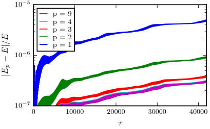
To further illustrate that no relevant short-time-scale physics was accidentally discarded by the use of an implicit integration scheme, we show in Fig. 19 the evolution of a representative mode mode for two rather distinct values of . The difference between these two figures is of order .
References
- [1] D. Christodoulou and S. Klainerman, Séminaire Équations aux dérivées partielles (Polytechnique) , 1 (1993).
- [2] H. Friedrich, Journal of Geometry and Physics 3, 101 (1986).
- [3] H. Friedrich, Class. Quant. Grav. 31, 105001 (2014), arXiv:1401.7172 [gr-qc] .
- [4] M. Dafermos and G. Holzegel, “Dynamic instability of solitons in 4+1 dimensional gravity with negative cosmological constant.” (unpublished).
- [5] M. T. Anderson, Class.Quant.Grav. 23, 6935 (2006), arXiv:hep-th/0605293 [hep-th] .
- [6] G. H. Holzegel and C. M. Warnick, (2013), arXiv:1312.5332 [gr-qc] .
- [7] P. Bizon and A. Rostworowski, Phys. Rev. Lett. 107, 031102 (2011), arXiv:1104.3702 [gr-qc] .
- [8] A. Buchel, L. Lehner, and S. L. Liebling, Phys. Rev. D86, 123011 (2012), arXiv:1210.0890 [gr-qc] .
- [9] O. J. Dias, G. T. Horowitz, D. Marolf, and J. E. Santos, Class. Quant. Grav. 29, 235019 (2012), arXiv:1208.5772 [gr-qc] .
- [10] M. Maliborski and A. Rostworowski, Phys. Rev. Lett. 111, 051102 (2013a), arXiv:1303.3186 [gr-qc] .
- [11] G. Fodor, P. Forgács, and P. Grandclément, (2015), arXiv:1503.07746 [gr-qc] .
- [12] V. Balasubramanian, A. Buchel, S. R. Green, L. Lehner, and S. L. Liebling, Phys. Rev. Lett. 113, 071601 (2014), arXiv:1403.6471 [hep-th] .
- [13] B. Craps, O. Evnin, and J. Vanhoof, JHEP 1410, 48 (2014), arXiv:1407.6273 [gr-qc] .
- [14] B. Craps, O. Evnin, and J. Vanhoof, JHEP 1501, 108 (2015), arXiv:1412.3249 [gr-qc] .
- [15] A. Buchel, S. R. Green, L. Lehner, and S. L. Liebling, Phys.Rev. D91, 064026 (2015), arXiv:1412.4761 [gr-qc] .
- [16] E. Fermi, J. Pasta, and S. M. Ulam, Studies of nonlinear problems. I, Technical Report LA-1940 (1955) also in Enrico Fermi: Collected Papers, volume 2, edited by Edoardo Amaldi, Herbert L. Anderson, Enrico Persico, Emilio Segré, and Albedo Wattenberg. Chicago: University of Chicago Press, 1965.
- [17] A. Buchel, S. L. Liebling, and L. Lehner, Phys. Rev. D87, 123006 (2013), arXiv:1304.4166 [gr-qc] .
- [18] O. Evnin and C. Krishnan, Phys. Rev. D91, 126010 (2015), arXiv:1502.03749 [hep-th] .
- [19] I.-S. Yang, Phys. Rev. D91, 065011 (2015), arXiv:1501.00998 [hep-th] .
- [20] H. Yang, F. Zhang, S. R. Green, and L. Lehner, Phys.Rev. D91, 084007 (2015), arXiv:1502.08051 [gr-qc] .
- [21] P. Basu, C. Krishnan, and A. Saurabh, (2014), arXiv:1408.0624 [gr-qc] .
- [22] S. Flach, M. Ivanchenko, and O. Kanakov, Phys. Rev. Lett. 95, 064102 (2005).
- [23] S. Flach, M. Ivanchenko, and O. Kanakov, Phys. Rev. E 73, 036618 (2006).
- [24] M. Maliborski and A. Rostworowski, Int. J. Mod. Phys. A28, 1340020 (2013b), arXiv:1308.1235 [gr-qc] .
- [25] F. Dimitrakopoulos and I.-S. Yang, (2015), arXiv:1507.02684 [hep-th] .
- [26] R. Cooke and V. I. Arnol’d, Ordinary Differential Equations, Springer Textbook (Springer Berlin Heidelberg, 1992).
- [27] N. Deppe, A. Kolly, A. Frey, and G. Kunstatter, (2014), arXiv:1410.1869 [hep-th] .
- [28] A. Buchel, S. R. Green, L. Lehner, and S. L. Liebling, (2014), arXiv:1410.5381 [hep-th] .
- [29] C. W. Misner, K. S. Thorne, and J. A. Wheeler, Gravitation (W. H. Freeman, San Francisco, 1973).
- [30] P. Basu, C. Krishnan, and P. N. Bala Subramanian, Phys. Lett. B746, 261 (2015), arXiv:1501.07499 [hep-th] .
- [31] P. Bizon, M. Maliborski, and A. Rostworowski, (2015), arXiv:1506.03519 [hep-th] .
- [32] A. Lichtenberg and M. Lieberman, Regular and chaotic dynamics, Applied mathematical sciences (Springer-Verlag, 1992).
- [33] M. Maliborski, Phys. Rev. Lett. 109, 221101 (2012), arXiv:1208.2934 [gr-qc] .
- [34] I. Gradshteyn and I. Ryzhik, “Table of integrals, series, and products,” (Academic Press Inc., 1980) 4th ed.