On Proportions of Fit Individuals in Population of Mutation-Based Evolutionary Algorithm with Tournament Selection
Abstract
In this paper, we consider a fitness-level model of a non-elitist mutation-only evolutionary algorithm (EA) with tournament selection. The model provides upper and lower bounds for the expected proportion of the individuals with fitness above given thresholds. In the case of so-called monotone mutation, the obtained bounds imply that increasing the tournament size improves the EA performance. As corollaries, we obtain an exponentially vanishing tail bound for the Randomized Local Search on unimodal functions and polynomial upper bounds on the runtime of EAs on 2-SAT problem and on a family of Set Cover problems proposed by E. Balas.
Sobolev Institute of Mathematics, Omsk Branch,
13 Pevtsov str., Omsk, 644099, Russia
eremeev@ofim.oscsbras.ru
1 Introduction
Evolutionary algorithms are randomized heuristic algorithms employing a population of tentative solutions (individuals) and simulating an evolutionary type of search for optimal or near-optimal solutions by means of selection, crossover and mutation operators. The evolutionary algorithms with crossover operator are usually called genetic algorithms (GAs). Evolutionary algorithms in general have a more flexible outline and include genetic programming, evolution strategies, estimation of distribution algorithms and other evolution-inspired paradigms. Evolutionary algorithms are now frequently used in areas of operations research, engineering and artificial intelligence.
Two major outlines of an evolutionary algorithm are the elitist evolutionary algorithm, that keeps a certain number of most promising individuals from the previous iteration, and the non-elitist evolutionary algorithm, that computes all individuals of a new population independently using the same randomized procedure. In this paper, we focus on the non-elitist case.
One of the first theoretical results in the analysis of non-elitist GAs is Schemata Theorem (Goldberg,, 1989) which gives a lower bound on the expected number of individuals from some subsets of the search space (schemata) in the next generation, given the current population. A significant progress in understanding the dynamics of GAs with non-elitist outline was made in (Vose,, 1995) by means of dynamical systems. However most of the findings in (Vose,, 1995) apply to the infinite population case, and it is not clear how these results can be used to estimate the applicability of GAs to practical optimization problems. A theoretical possibility of constructing GAs that provably optimize an objective function with high probability in polynomial time was shown in (Vitányi,, 2000) using rapidly mixing Markov chains. However (Vitányi,, 2000) provides only a very simple artificial example where this approach is applicable and further developments in this direction are not known to us.
One of the standard approaches to studying evolutionary algorithms in general, is based on the fitness levels (Wegener,, 2002). In this approach, the solution space is partitioned into disjoint subsets, called fitness-levels, according to values of the fitness function. In (Lehre,, 2011), the fitness-level approach was first applied to upper-bound the runtime of non-elitist mutation-only evolutionary algorithms. Here and below, by the runtime we mean the expected number of fitness evaluations made until an optimum is found for the first time. Upper bounds of the runtime of non-elitist GAs, involving the crossover operators, were obtained later in (Corus et al.,, 2014; Eremeev,, 2016). The runtime bounds presented in (Corus et al.,, 2014; Lehre,, 2011) are based on the drift analysis. In (Moraglio and Sudholt,, 2015), a runtime result is proposed for a class of convex search algorithms, including some non-elitist crossover-based GAs without mutation, on the so-called concave fitness landscapes.
In this paper, we consider the non-elitist evolutionary algorithm which uses a tournament selection and a mutation operator but no crossover. The -tournament selection randomly chooses individuals from the existing population and selects the best one of them (see e.g. (Thierens and Goldberg,, 1994)). The mutation operator is viewed as a randomized procedure, which computes one offspring with a probability distribution depending on the given parent individual. In this paper, evolutionary algorithms with such outline are denoted as EA. We study the probability distribution of the EA population w.r.t. a set of fitness levels. The estimates of the EA behavior are based on a priori known parameters of a mutation operator. Using the proposed model we obtain upper and lower bounds on expected proportion of the individuals with fitness above certain thresholds. The lower bounds are formulated in terms of linear algebra and resemble the bound in Schemata Theorem (Goldberg,, 1989). Instead of schemata here we consider the sets of genotypes with the fitness bounded from below. Besides that, the bounds obtained in this paper may be applied recursively up to any given iteration.
A particular attention in this paper is payed to a special case when mutation is monotone. Informally speaking, a mutation operator is monotone if throughout the search space the following condition holds: the greater the fitness of a parent the “better” offspring distribution the mutation generates. One of the most well-known examples of monotone mutation is the bitwise mutation in the case of OneMax fitness function. As shown in (Borisovsky and Eremeev,, 2008), in the case of monotone mutation, one of the most simple evolutionary algorithms, known as the (+) EA has the best-possible performance in terms of runtime and probability of finding the optimum.
In the case of monotone mutation, the lower bounds on expected proportions of the individuals turn into equalities for the trivial evolutionary algorithm (,) EA. This implies that the tournament selection at least has no negative effect on the EA performance in such a case. This observation is complemented by the asymptotic analysis of the EA with monotone mutation indicating that, given a sufficiently large population size and some technical conditions, increasing the tournament size always improves the EA performance.
As corollaries of the general lower bounds on expected proportions of sufficiently fit individuals, we obtain polynomial upper bounds on the Randomized Local Search runtime on unimodal functions and upper bounds on runtime of EAs on 2-SAT problem and on a family of Set Cover problems proposed by Balas, (1984). Unlike the upper bounds on runtime of evolutionary algorithms with tournament selection from (Corus et al.,, 2014; Eremeev,, 2016; Lehre,, 2011), which require sufficiently large tournament size, the upper bounds on runtime obtained here hold for any tournament size.
The rest of the paper is organized as follows. In Section 2, we give a formal description of the considered EA, introduce an approximating model of the EA population and define some required parameters of the probability distribution of a mutation operator in terms of fitness levels. In Section 3, using the model from Section 2, we obtain lower and upper bounds on expected proportions of genotypes with fitness above some given thresholds. Section 4 is devoted to analysis of an important special case of monotone mutation operator, where the bounds obtained in the previous section become tight or asymptotically tight. In Section 5, we consider some illustrative examples of monotone mutation operators and demonstrate some applications of the general results from Section 3. In particular, in this section we obtain new lower bounds for probability to generate optimal genotypes at any given iteration for a class of unimodal functions, for 2-SAT problem and for a family of set cover problems proposed by E. Balas (in the latter two cases we also obtain upper bounds on the runtime of the EA). Besides that in Section 5 we give an upper bound on expected proportion of optimal genotypes for OneMax fitness function. Section 6 contains concluding remarks.
This work extends the conference paper (Eremeev,, 2000). The extension consists in comparison of the EA behavior to that of the (,) EA, the (,) EA and the (+) EA in Section 3 and in the new runtime bounds and tail bounds demonstrated in Section 5. The main results from the conference paper are refined and provided with more detailed proofs.
2 Description of Algorithms and Approximating Model
2.1 Notation and Algorithms
Let the optimization problem consist in maximization of an objective function on the set of feasible solutions , where is the search space of all binary strings of length .
The Evolutionary Algorithm EA.
The EA searches for the optimal or sub-optimal solutions using a population of individuals, where each individual (genotype) is a bitstring , and its components are called genes.
In each iteration the EA constructs a new population on the basis of the previous one. The search process is guided by the values of a fitness function
where is a penalty function.
The individuals of the population may be ordered according to the sequence in which they are generated, thus the population may be considered as a vector of genotypes , where is the size of population, which is constant during the run of the EA, and is the number of the current iteration. In this paper, we consider a non-elitist algorithmic outline, where all individuals of a new population are generated independently from each other with identical probability distribution depending on the existing population only.
Each individual is generated through selection of a parent genotype by means of a selection operator, and modification of this genotype in mutation operator. During the mutation, a subset of genes in the genotype string is randomly altered. In general the mutation operator may be viewed as a random variable with the probability distribution depending on .
The genotypes of the initial population are generated with some a priori chosen probability distribution. The stopping criterion may be e.g. an upper bound on the number of iterations . The result is the best solution generated during the run. The EA has the following scheme.
1. Generate the initial population .
2. For to do
2.1. For to do
Choose a parent genotype from
by -tournament selection.
Add to the
population .
In theoretical studies, the evolutionary algorithms are usually treated without a stopping criterion (see e.g. (Neumann and Witt,, 2010)). Unless otherwise stated, in the EA we will also assume that
Note that in the special case of the EA with we can assume that , since the tournament selection has no effect in this case.
(,) EA and (+) EA.
In the following sections we will also need a description of two simple evolutionary algorithms, known as the (,) EA and the (+) EA.
The genotype of the current individual on iteration of the (,) EA will be denoted by , and in the (+) EA it will be denoted by . The initial genotypes and are generated with some a priori chosen probability distribution. The only difference between the (,) EA and the (+) EA consists in the method of construction of an individual for iteration using the current individual of iteration as a parent. In both algorithms the new individual is built with the help of a mutation operator, which we will denote by . In case of the (,) EA, the mutation operator is independently applied times to the parent genotype and out of offspring a single genotype with the highest fitness value is chosen as . (If there are several offspring with the highest fitness, the new individual is chosen arbitrarily among them.) In the (+) EA, the mutation operator is applied to once. If is such that then ; otherwise .
2.2 The Proposed Model
The EA may be considered as a Markov chain in a number of ways. For example, the states of the chain may correspond to different vectors of genotypes that constitute the population (see (Rudolph,, 1994)). In this case the number of states in the Markov chain is . Another model representing the GA as a Markov chain is proposed in (Nix and Vose,, 1992), where all populations which differ only in the ordering of individuals are considered to be equivalent. Each state of this Markov chain may be represented by a vector of components, where the proportion of each genotype in the population is indicated by the corresponding coordinate and the total number of states is . In the framework of this model, M.Vose and collaborators have obtained a number of general results concerning the emergent behavior of GAs by linking these algorithms to the infinite-population GAs (Vose,, 1995).
The major difficulties in application of the above mentioned models to the analysis of GAs for combinatorial optimization problems are connected with the necessity to use the high-grained information about fitness value of each genotype. In the present paper, we consider one of the ways to avoid these difficulties by means of grouping the genotypes into larger classes on the basis of their fitness.
Assume that and there are level lines of the fitness function fixed such that . The number of levels and the fitness values corresponding to them may be chosen arbitrarily, but they should be relevant to the given problem and the mutation operator to yield a meaningful model. Let us introduce the sequence of Lebesgue subsets of
Obviously, . For the sake of convenience, we define . Also, we denote the level sets which give a partition of . Partitioning subsets are more frequently used in literature on level-based analysis, compared to the Lebesgue subsets . In this paper we will frequently state that a genotype has a sufficiently high fitness, therefore the use of subsets will be more convenient in such cases. One of the partitions used in the literature, called the canonical partition, defines as the set of all fitness values on the search space .
Now suppose that for all and the a priori lower bounds and upper bounds on mutation transition probabilities from subset to are known, i.e.
Fig. 1 illustrates the transitions considered in this expression.

Let A denote the matrix with the elements where , and . The similar matrix of upper bounds is denoted by B. Let the population on iteration be represented by the population vector
where is the proportion of genotypes from in population . The population vector is a random vector, where for since .
Let be the probability that an individual, which is added after selection and mutation into , has a genotype from for , and According to the scheme of the EA this probability is identical for all genotypes of , i.e. .
Proposition 1
for all .
Proof. Consider the sequence of identically distributed random variables , where if the -th individual in the population belongs to , otherwise . By the definition, , consequently
Level-Based Mutation.
If for some mutation operator there exist two equal matrices of lower and upper bounds A and B, i.e. for all then the mutation operator will be called level-based. By this definition, in the case of level-based mutation, does not depend on a choice of genotype and the probabilities are well-defined. In what follows, we call a cumulative transition probability. The symbol will denote the matrix of cumulative transition probabilities of a level-based mutation operator.
If the EA uses a level-based mutation operator, then the probability distribution of population is completely determined by the vector . In this case the EA may be viewed as a Markov chain with states corresponding to the elements of
which is the set of all possible vectors of population of size . Here and below, the symbol z is used to denote a vector from the set of all possible population vectors .
The cardinality of set may be evaluated analogously to the number of states in the model of Nix and Vose, (1992). Now levels replace individual elements of the search space, which gives a total of possible population vectors.
3 Bounds on Expected Proportions of Fit Individuals
In this section, our aim is to obtain lower and upper bounds on for arbitrary and if the distribution of the initial population is known.
Let denote the probability that the genotype, chosen by the tournament selection from a population with vector z, belongs to a subset . Note that if the current population is represented by the vector , then a genotype obtained by selection and mutation would belong to with a conditional probability
| (1) |
3.1 Lower Bounds
Expression (1) and the definitions of bounds yield for all :
| (2) |
which turns into an equality in the case of level-based mutation and .
Given a tournament size we obtain the following selection probabilities: , and, consequently, . This leads to the inequality:
By the total probability formula,
| (3) |
| (4) |
where the last expression is obtained by regrouping the summation terms. Proposition 1 implies that . Consequently, since and , expression (4) gives a lower bound
| (5) |
Note that (5) turns into an equality in the case of level-based mutation and . We would like to use (5) recursively times in order to estimate for any , given the initial vector . It will be shown in the sequel that such a recursion is possible under monotonicity assumptions defined below.
Monotone Matrices and Mutation Operators.
In what follows, any -matrix with elements , will be called monotone iff for all from 1 to . Monotonicity of a matrix of bounds on transition probabilities means that the greater fitness level a parent solution has, the greater is its bound on transition probability to any subset . Note that for any mutation operator the monotone upper and lower bounds exist. Formally, for any mutation operator a valid monotone matrix of lower bounds would be where is a zero matrix. A monotone matrix of upper bounds, valid for any mutation operator is , where is the matrix with all elements equal 1. These are extreme and impractical examples. In reality a problem may be connected with the absence of bounds which are sharp enough to evaluate the mutation operator properly.
If given some set of levels there exist two matrices of lower and upper bounds such that and these matrices are monotone then operator is called monotone w.r.t. the set of levels . In this paper, we will also call such operators monotone for short. Note that by the definition, any monotone mutation operator is level-based, since for all . The following proposition shows how the monotonicity property may be equivalently defined in terms of cumulative transition probabilities.
Proposition 2
A mutation operator is monotone w.r.t. the set of levels iff for any such that for any genotypes holds
Proof. Indeed, suppose that and these matrices are monotone. Then for any genotypes and , holds
Conversely, if for any level and any genotypes and
, holds , then taking we note that
is equal for all and one
can assign The resulting matrices A and B are obviously
monotone.
Proposition 2 implies that in the case of the canonical partition, i.e. when is the set of all values of , operator is monotone w.r.t. iff for any genotypes and such that , for any holds
The monotonicity of mutation operator w.r.t. a canonical partition is equivalent to the definition of monotone reproduction operator from (Borisovsky and Eremeev,, 2001) in the case of single-parent, single-offspring reproduction. According to the terminology of Daley, (1968), such random operators are also called stochastically monotone.
As a simple example of a monotone mutation operator we can consider a point mutation operator: with probability keep the given genotype unchanged; otherwise (with probability ) choose randomly from and change gene . As a fitness function we take the function , where . Let us assume and define the thresholds . All genotypes with the same fitness function value have equal probability to produce an offspring with any required fitness value, therefore this is a case of level-based mutation. In such a case identical matrices of lower and upper bounds A and B exist and they both equal to the matrix of cumulative transition probabilities . The latter consists of the following elements: for all , since point mutation can not reduce the fitness by more than one level; for because with probability any genotype is upgraded;
because a genotype in can be obtained as an offspring of a genotype from in two ways: either the parent genotype has been upgraded (which happens with probability ) or it stays at level , which happens with probability ; finally because point mutation can not increase the level number by more than 1. The elements of matrix obviously satisfy the monotonicity condition when . For the case of we have which is nonnegative if Therefore with any the matrix is monotone in this example and the mutation operator is monotone as well.
Proposition 3
If A is monotone, then for any tournament size and holds
| (6) |
besides that (6) is an equality if , operator is monotone and A is its matrix of cumulative transition probabilities.
Proof. Monotonicity of matrix A implies that for all so the simple estimate may be applied to all terms of the sum in (5) and we get
Regrouping the terms in the last bound we obtain the required inequality (6).
Finally, note that lower bound (5) holds as an equality if the mutation operator is monotone and , therefore the last lower bound is an equality in the case of monotone and .
Lower Bounds from Linear Algebra.
Let be a -matrix with elements let be the identity matrix of the same size, and denote . With these notations, inequality (6) takes a short form Here and below, the inequality sign ”” for some vectors and means the component-wise comparison, i.e. iff for all . The following theorem gives a component-wise lower bound on vector for any .
Theorem 1
Suppose that is some matrix norm. If matrix A is monotone and , then for all holds
| (7) |
and inequality (7) turns into an equation if the tournament size , the mutation operator used in the EA is monotone and A is its matrix of cumulative transition probabilities.
The proof of this theorem is similar to the well-known inductive
proof of the formula for a sum of terms in a geometric
series Note that the recursion is similar to the recursive formula
assuming . However in our case
matrices and vectors replace numbers, we have to deal with
inequalities rather than equalities and the initial
element may be non-zero unlike .
Proof of Theorem 1. Let us consider a sequence of -dimensional vectors , where , . We will show that for any , using induction on . Indeed, for the inequality holds by the definition of . Now note that the right-hand side of (6) will not increase if the components of are substituted with their lower bounds. Therefore, assuming we already have for some and substituting for we make an inductive step .
By properties of the linear operators (see e.g. (Kolmogorov and Fomin,, 1999), Chapter III, § 29), due to the assumption that we conclude that matrix exists.
Now, using the induction on for any we will obtain the identity
which leads to inequality (7). Indeed, for the base case of by the definition of we have the required equality. For the inductive step, we use the following relationship
In conditions of Theorem 1, the right-hand side of (7) approaches when tends to infinity, thus the limit of this bound does not depend on distribution of the initial population.
In many evolutionary algorithms, an arbitrary given genotype may be produced with a non-zero probability as a result of mutation of any given genotype . Suppose that the probability of such a mutation is lower bounded by some for all . Then one can obviously choose some monotone matrix A of lower bounds that satisfies for all . Thus, for all . In this case one can consider the matrix norm . Due to monotonicity of A we have , so , and the conditions of Theorem 1 are satisfied. A trivial example of a matrix that satisfies the above description would be a matrix A where all elements are equal to .
Application of Theorem 1 may be complicated due to difficulties in finding the vector and in estimation the effect of multiplication by matrix Some known results from linear algebra can help to solve these tasks, as the example in Subsection 5.2 shows. However sometimes it is possible to obtain a lower bound for via analysis of the (,) EA algorithm, choosing an appropriate mutation operator for it. This approach is discussed below.
Lower Bounds from Associated Markov Chain.
Suppose that a partition defined by contains no empty subsets and let T denote a -matrix, with components
Note that T is a stochastic matrix so it may be viewed as a transition matrix of a Markov chain, associated to the set of lower bounds . This chain is a model of the (,) EA, which is a special case of the (,) EA with (see Subsection 2.1). Suppose that the (,) EA uses an artificial monotone mutation operator where the cumulative transition probabilities are defined by the bounds , corresponding to the EA mutation operator . Namely, given a parent genotype , for any we have , where is such that . Operator may be simulated e.g. by the following two-stage procedure. At the first stage, a random index of the offspring level is chosen with the probability distribution where is the level of parent . At the second stage, the offspring genotype is drawn uniformly at random from . (Simulation of the second stage may be computationally expensive for some fitness functions but the complexity issues are not considered now.) The initial search point of the (,) EA is generated at random with probability distribution defined by the probabilities . Denoting , by properties of Markov chains we get . The following theorem is based on a comparison of to the distribution of the Markov chain .
Theorem 2
Suppose all level subsets are non-empty and matrix A is monotone. Then for any holds
| (8) |
where is a triangular -matrix with components if and otherwise. Besides that inequality (8) turns into an equation if , the EA mutation operator is monotone and A is its matrix of cumulative transition probabilities.
Proof. The (,) EA described above is identical to an EA’ with , and mutation operator . Let us denote the population vector of EA’ by . Obviously,
| (9) |
Proposition 3 implies that in the original EA with population size and tournament size , the expectation is lower bounded by the expectation since (6) holds as an equality for the whole sequence of and the right-hand side of (6) is non-decreasing on . Equality together with (9) imply the required bound (8).
3.2 Upper Bounds
In this subsection, we obtain upper bounds on using a reasoning similar to the proof of Proposition 3. Expression (1) for all yields:
| (10) |
which turns into equality in the case of level-based mutation. By the total probability formula we have:
| (11) |
so
| (12) |
Under the expectation in the right-hand side we have a convex function on . Therefore, in the case of monotone matrix B, using Jensen’s inequality (see e.g. (Rudin,, 1987), Chapter 3) we obtain the following proposition.
Proposition 4
If B is monotone then
| (13) |
By means of iterative application of inequality (13) the components of the expected population vectors may be bounded up to arbitrary , starting from the initial vector . The nonlinearity in the right-hand side of (13), however, creates an obstacle for obtaining an analytical result similar to the bounds of Theorems 1 and 2.
3.3 Comparison of EA to (,) EA and (+) EA
This subsection shows how the probability of generating the optimal genotypes at a given iteration of the EA relates to analogous probabilities of (,) EA and (+) EA. The analysis here will be based on upper bound (13) and on some previously known results provided in the attachment.
Suppose, matrix B gives the upper bounds for cumulative transition probabilities of the mutation operator used in the EA. Consider the (,) EA and the (+) EA, based on a monotone mutation operator for which B is the matrix of cumulative transition probabilities and suppose that the initial solutions and have the same distribution over the fitness levels as the best incumbent solution in the EA population . Formally: for any and In what follows, for any by we denote the probability that current individual on iteration of the (,) EA belongs to . Analogously denotes the probability for the (+) EA.
The following proposition is based on upper bound (13) and the results from (Borisovsky,, 2001; Borisovsky and Eremeev,, 2001) that allow to compare the performance of the EA, the (,) EA and the (+) EA.
Proposition 5
Suppose that matrix B is monotone. Then for any holds
Proof. Let us compare the EA to the (,) EA and to the
(+) EA using the mutation and initialization procedures as
described above. Theorem 6 (see the appendix) together
with Proposition 1 imply that
for
all . Furthermore, Theorem 5 from (Borisovsky and Eremeev,, 2001) (see the
appendix) implies that for
all . Using Proposition 4 and
monotonicity of B, we conclude that both claimed inequalities
hold.
4 EA with Monotone Mutation Operator
First of all note that in the case of monotone mutation operator, two equal monotone matrices of lower and upper bounds exist, so the bounds (5) and (12) give equal results, and assuming we get
| (14) |
This equality will be used several times in what follows.
In general, the population vectors are random values whose distributions depend on . To express this in the notation let us denote the proportion of genotypes from in population by .
The following Lemma 1 and Theorem 3 based on this lemma indicate that in the case of monotone mutation, recursive application of the formula from right-hand side of upper bound (13) allows to compute the expected population vector of the infinite-population EA at any iteration .
Lemma 1
Let the EA use a monotone mutation operator with cumulative transition probabilities matrix , and let the genotypes of the initial population be identically distributed. Then
(i) for all and holds
| (15) |
(ii) if the sequence of -dimensional vectors is defined as
| (16) |
| (17) |
for and . Then for all at any iteration .
The main step in the proof of Lemma 1 (i) will consist in showing that for a supplementary random variable the value of is upper-bounded by an arbitrary small . This step is made by splitting the range of into a “high-probability” area and a “low-probability” area in such a way that is at most in the “high-probability” area. Analogous technique is used e.g. in the proof of Lebesgue Theorem, see e.g. Kolmogorov and Fomin, (1999), Chapter VII, § 44.
Proof of Lemma 1. From (14), we conclude that if statement (i) holds, then with the convergence of to will imply that . Thus, statement (ii) follows by induction on .
Let us now prove statement (i). Given some to prove (15) we recall the sequence of i.i.d. random variables , where , if the -th individual of population belongs to , otherwise . By the law of large numbers, for any and , we have
Note that . Besides that, due to Proposition 1, (In the case of this equality holds as well, since all individuals of the initial population are distributed identically.) Therefore, for any the convergence holds. Now by continuity of the function , it follows that
Let us denote . Then
for arbitrary , hence (15) holds.
Combining equality (14) with claim (i) of Lemma 1 we obtain a recursive expression for in the infinite-population EA, which is formulated as
Theorem 3
If the mutation operator is monotone and individuals of the initial population are distributed identically, then
| (18) |
for all .
For any and the term of the sequence defined by (17) is nondecreasing in and in as well. With this in mind, we can expect that the components of population vector of the infinite-population EA will typically increase with the tournament size. Theorem 4 below gives a rigorous proof of this fact under some technical conditions on distributions of and .
Theorem 4
Let and correspond to EAs with tournament sizes and , where . Besides that, suppose that is monotone with for all and the individuals of initial populations are identically distributed so that for all . Then for any , given a sufficiently large holds
Proof. Let the sequences and be defined as in Lemma 1, corresponding to tournament sizes and . By the above assumptions,
Now since for all we have for any . Thus, for all holds
| (19) |
since and at least for one of the levels according to the assumption that . Due to the same reason, for all from the last equality in (19) we get Using the fact that and re-arranging the terms as in the proof of Proposition 3 we get
To sum up, for we have and .
Furthermore, if we assume that for all holds and then analogously to (19) we get for all . Besides that, just as in the case of we get and So by induction we conclude that for all and all .
Finally, by claim (ii) of Lemma 1, for any and ,
given a sufficiently large , holds
.
Informally speaking, Theorem 4 implies that in the case of monotone mutation operator an optimal selection mechanism consists in setting which actually converts the EA into the (,) EA.
5 Applications and Illustrative Examples
5.1 Examples of Monotone Mutation Operators
Let us consider two cases where the mutation is monotone and the matrices have a similar form.
First we consider the simple fitness function . Suppose that the EA uses the bitwise mutation operator, changing every gene with a given probability , independently of the other genes. Let the subsets be defined by the level lines and . The matrix for this operator could be obtained using the result from (Bäck,, 1993), but here we shall consider this example as a special case of a more general setting.
Let the representation of the problem admit a decomposition of the genotype string into non-overlapping substrings (called blocks here) in such a way that the fitness function equals the number of blocks for which a certain property holds. The functions of this type belong to the class of additively decomposed functions, where the elementary functions are Boolean and substrings are non-overlapping (see e.g. (Mühlenbein et al.,, 1999)). Let if holds for the block of genotype , and otherwise (here ).
Suppose that during mutation, any block for which did not hold, gets the property with probability , i.e.
On the other hand, assume that a block with the property keeps this property during mutation with probability , i.e.
Let and the subsets correspond to the level lines again. In this case the element of cumulative transition probabilities matrix equals the probability to obtain a genotype containing or more blocks with property after mutation of a genotype which contained blocks with this property. Let denote the probability that during mutation blocks without property would produce blocks with this property and let denote the probability that after mutation of a set of blocks with property , there will be at least blocks with property among them. (If then ) With these notations,
Clearly, and Thus,
| (20) |
It is shown in (Eremeev,, 2000; Borisovsky and Eremeev,, 2008) that if then matrix defined by (20) is monotone.
Now matrix for the bitwise mutation on OneMax function is obtained assuming that and . This operator is monotone in view of the above mentioned result, if , since in this case . The monotonicity of bitwise mutation on OneMax is used in works of Doerr et al., (2010) and Witt, (2013).
Expression (20) may be also used for finding the cumulative transition matrices of some other optimization problems with a regular structure. As an example, below we consider the vertex cover problem (VCP) on graphs of a special structure.
In general, the vertex cover problem is formulated as follows. Let be a graph with a set of vertices and the edge set where . A subset is called a vertex cover of if every edge has at least one endpoint in . The vertex cover problem is to find a vertex cover of minimal cardinality.
Suppose that the VCP is handled by the EA with the following representation: each gene corresponds to an edge of , assigning one of its endpoints which has to be included in the cover . To be specific, we can assume that means that and means that . The vertices, not assigned by one of the chosen endpoints, do not belong to . On one hand, this edge-based representation is degenerate in the sense that one vertex cover may be encoded by different genotypes . On the other hand, any genotype defines a feasible cover . A natural way to choose the fitness function in the case of this representation is to assume .
Note that most publications on evolutionary algorithms for VCP use the vertex-based representation with genes, where implies inclusion of vertex into (see e.g. (Neumann and Witt,, 2010), § 12.1). In contrast to the edge-based representation, the vertex-based representation is not degenerate but some genotypes in this representation may define infeasible solutions.
Following (Saiko,, 1989) we denote by the graph consisting of disconnected triangle subgraphs. Each triangle is covered optimally by two vertices and the redundant cover consists of three vertices. In spite of simplicity of this problem, it is proven in (Saiko,, 1989) that some well-known algorithms of branch and bound type require exponential in number of iterations if applied to the VCP on graph .
In the case of , the fitness coincides with the number of optimally covered triangles in (i.e. triangles where only two different vertices are chosen), since covering non-optimally all triangles gives and each optimally covered triangle decreases the size of the cover by one. Let the genes representing the same triangle constitute a single block, and let the property imply that a triangle is optimally covered. Then by looking at the two possible ways to produce a gene triplet that redundantly covers a triangle, (i) given a redundant triangle and (ii) given an optimally covered triangle, we conclude that (i) and (ii) . Using (20) we obtain the cumulative transition matrix for this mutation operator. It is easy to verify that in this case the inequality holds for any mutation probability , and therefore the operator is always monotone.
Computational Experiments.
Below we present some experimental results in comparison with the theoretical estimates obtained in Section 3. To this end we consider an application of the EA to the VCP on graphs . The average proportion of optimal genotypes in the population for different population sizes is presented in Figure 2. Here , , and (these parameters are chosen to ensure clear visibility on plots). The statistics is accumulated in 1000 independent runs of the algorithm where for each only one individual was checked for optimality. Thus for each we have a series of 1000 Bernoully trials with a success probability which is estimated from the experimental data. The 95%-confidence intervals for success probability in Bernoully trials are computed using the Normal approximation as described in (Cramer,, 1946), Chapter 34.
The experimental results are shown in dashed lines. The solid lines correspond to the lower and upper bounds given by the expressions (7) and (13). The plot shows that upper bound (13) gives a good approximation to the value of even if the population size is not large. The lower bound (7) coincides with the experimental results when , up to a minor sampling error.
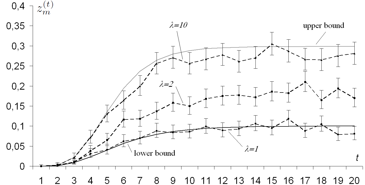
Another series of experiments was carried out to compare the behavior of EAs with different tournament sizes. Figure 3 presents the experimental results for 1000 runs of the EA with , and solving the VCP on . This plot demonstrates the increase in the average proportion of the optimal genotypes as a function of the tournament size, which is consistent with Theorem 4. The 95%-confidence intervals are found as described above.

5.2 Lower Bound for Randomized Local Search on Unimodal Functions.
First of all let us describe a Randomized Local Search algorithm (RLS) which will be implicitly studied in this subsection. At each iteration of RLS the current genotype is stored. In the beginning of RLS execution, is initialized with some probability distribution (e.g. uniformly over ). An iteration of RLS consists in building an offspring of by flipping exactly one randomly chosen bit in . If then is replaced by the new genotype . The process continues until some termination condition is met.
Below we will illustrate the usage of Theorem 1 on the class of -Unimodal functions. In this class, each function has exactly distinctive fitness values , and each solution in the search space is either optimal or its fitness may be improved by flipping a single bit. Naturally we assume that and that level consists of optimal solutions.
As a mutation operator in the EA we will use a routine denoted by : given a genotype , this routine first changes one randomly chosen gene and if this modification improves the genotype fitness, then outputs the modified genotype, otherwise outputs the genotype unchanged. Note that in the case of the EA with mutation becomes a version of RLS. The lower bounds from Section 3 are tight for (which implies ), therefore the following analysis in this subsection may be viewed primarily as a study of Randomized Local Search.
Mutation operator never decreases the genotype fitness and improves any non-optimal genotype with probability at least , so we have for all and for . The chances for improvements by more that one fitness level are not foreseeable, so we put for all . Note that this matrix A is monotone.
Now and the matrix consists of the following elements:
In order to apply Theorem 1 we also need to choose an appropriate matrix norm and evaluate this norm for matrix . In this particular application we will use which is the matrix norm induced by the Euclidean vector norm in . It is well-known that for any matrix holds where is the maximal eigenvalue of matrix Here and below denotes the transpose of matrix
It is easy to check that matrix is composed of zero elements everywhere except for diagonal elements, superdiagonal and subdiagonal elements. In particular, it has identical elements on the diagonal and all superdiagonal and subdiagonal elements are equal to . This matrix belongs to the class of tridiagonal Toeplitz matrices and its maximal eigenvalue is
(see Theorem 7 in the appendix). Therefore
So and since matrix A is monotone we can apply Theorem 1.
Let us denote . The vector satisfies the equation and since , the right-hand side in inequality (7) of Theorem 1 tends to as .
In order to obtain an explicit lower bound on for any given , we will evaluate the speed of convergence of the right-hand side in inequality (7) to e. Note that by properties of matrix norms we have
| (21) |
Thus for any distribution of initial population Theorem 1 gives a lower bound
where the last inequality holds because each component of vector is upper-bounded by which is at most by inequality (21).
Finally, independently of population size and tournament size we get a lower bound for the proportion of optimal genotypes in the EA population:
| (22) |
The Taylor expansion for gives
Now since and we obtain
In the case of RLS, i.e. when , this gives the following tail bound
Corollary 1
The probability that the maximum of a fitness function from -Unimodal is first reached after more than iterations of RLS is at most .
A positive feature of this tail bound is that it approaches to 0 exponentially fast in . A weakness of Corollary 1 is that its bound is grater than 1 (and therefore useless) when The obtained tail bound may be improved for some relatively small using the expected RLS runtime bound and Markov inequality. Let denote the number of fitness evaluations made in RLS until the optimum is achieved. Then the RLS runtime since each fitness level requires on average at most iterations of RLS. By Markov inequality we have . This tail bound becomes meaningful as soon as reaches but it does not give an exponential convergence and therefore yields to Corollary 1 for large . It would be interesting to compare our tail bounds to those obtainable by the approach from (Lehre and Witt,, 2014) but tight analysis of RLS is beyond the scope of this paper.
5.3 Lower Bounds and Runtime Analysis for 2-SAT Problem
The Satisfiability problem (SAT) in general is known to be NP-complete (Garey and Johnson,, 1979), but it is polynomially solvable in the special case denoted by 2-SAT: given a Boolean formula with CNF where each clause contains at most two literals, find out whether a satisfying assignment of variables exists.
Let be the number of logical variables and let be the number of clauses in the CNF. A natural encoding of solutions is a binary string where if the -th logical variable has the value ”true” and otherwise
We consider an EA with the tournament size and the following mutation operator : Draw randomly a clause which is not satisfied, choose one variable among the variables of the clause at random, and modify this variable. Otherwise keep the solution unchanged. This method of random perturbation was proposed in the randomized algorithm of Papadimitriou, (1991) for 2-SAT which has the runtime if the CNF is satisfiable. A generalization of the algorithm from (Papadimitriou,, 1991) to the general case of SAT, known as WalkSat algorithm, shows competitive experimental results (Selman et al.,, 1996). In the special case of SAT, where each clause contains at most literals, which is denoted by -SAT, algorithm WalkSat has a runtime bound (Schöning,, 1999).
A fitness function does not influence the EA execution when but it will be useful for our theoretical analysis. Let us assume that equals the Hamming distance to a satisfying assignment . Here and below, we assume that at least one satisfying assignment exists.
For any non-satisfying truth assignment the improvement probability is 1/2, so we can apply the following monotone bounds: for all ; for ;
. These lower bounds define the Markov chain transition probabilities T with and according to Subsection 3.1. It turns out that this matrix T is the same as the transition matrix of the symmetric Gambler’s Ruin random walk with one reflecting barrier (state 0) and one absorbing barrier (state ): for , , all other elements are equal to zero. The result from (Papadimitriou,, 1991) implies that, regardless of the initial state, there exists a constant , such that after transitions the absorbing probability of this random walk is at least 1/2. This means that and the -th component of the vector is at least as well. Therefore Theorem 2 yields
Corollary 2
If the EA for 2-SAT has the tournament size and the mutation operator then the probability to generate a satisfying assignment in population is at least for some constant
It makes sense to apply Theorem 2 only in the case of in this example, since for the tournament selection is impossible without computing the Hamming distance to a satisfying assignment which is unknown.
If the EA with and mutation is restarted every iterations and , then the overall runtime of this iterated EA is by Corollary 2 and Markov inequality. Note that Corollary 2 holds for any distribution of the initial population, so the runtime bound applies to the EA without restarts as well. In a similar way the EA with can simulate the randomized algorithm of Schöning (Schöning,, 1999) for -SAT with runtime .
5.4 Lower Bounds and Runtime Analysis for Balas Set Cover Problems
In general the set cover problem (SCP) is formulated as follows. Given: a ground set and a set of covering subsets , with indices . A subset of indices is called a cover if The goal is to find a cover of minimum cardinality. In what follows, for any we denote by the set of numbers of the subsets that cover an element , i. e. . Note that an instance of SCP may be defined by a family of subsets or, alternatively, by a family of subsets .
Suppose the binary representation of the SCP solutions is used, i.e. genes are the indicators of the elements from , so that . If is a cover then we assign its fitness ; otherwise , where is a decreasing function of the number of non-covered elements from
Consider a family of set cover problems introduced by Balas, (1984). Here it is assumed that and that all -element subsets of are given as subsets . Thus any collection of less than elements from belongs to for some and does not cover the element . At the same time any subset of size covers all elements of and therefore it is an optimal cover. Larger subsets are non-optimal covers.
Since any -element subset of is an optimal cover, family is solvable trivially. Nevertheless this family is known to be hard for general-purpose integer programming algorithms (Balas,, 1984; Saiko,, 1989). In particular, it was shown in (Saiko,, 1989) that problems from this class are hard to solve using the -class enumeration method (Kolokolov,, 1996). When is even and , the -class enumeration method needs an exponential number of iterations in . In what follows we analyze the EA in this special case.
Note that any -element subset for leaves elements of the ground set uncovered, regardless of the choice of elements in . So in the case of tournament selection, equivalently to studying the EA on family we may study the EA where the fitness is given by a function of unitation, so that
where function is decreasing, function is increasing and
Consider the point mutation operator with tunable parameter defined in Subsection 3.1. Let and let the thresholds be equal to fitness of genotypes that contain genes ”1” accordingly. Note that is a cover iff .
We have the following lower bounds: for all ; for ;
. These lower bounds coincide with the corresponding cumulative transition probabilities except for level , where we pessimistically assume (in fact we could safely put but is chosen to match the model of Ehrenfests in what follows). It is easy to verify that A satisfies the monotonicity condition when just as we verified this in the example of monotone mutation in Subsection 3.1.
In case we are interested in runtime bounds for the EA, rather than expected values of vector , we can assume . All other non-zero lower bounds defined above could be relaxed by putting . In this case we would have the associated Markov chain with a transition matrix the same as in Subsection 5.3, resulting in the same EA runtime bound . We shall avoid these simplifications, however, in order to obtain a tighter runtime bound by means of the following corollary.
Corollary 3
Suppose that the EA with a tournament size uses the point mutation operator with parameter . Then given there exists a constant , such that the probability to reach an optimum of problem within iterations is
To prove this corollary, first we will obtain a lower bound on for , using Theorem 2 and the stationary distribution of the associated Markov chain After that, analogously to the proof of Corollary 1, we will compute a lower bound on for finite , using Theorem 1.
Proof of Corollary 3. The Markov chain associated to the set of lower bounds defined above has the following nonzero transition probabilities
All other elements of matrix T are equal to zero.
The stationary distribution of the associated Markov chain may be found from the well-known model for diffusion of P. Ehrenfest and T. Ehrenfest. Consider molecules in a rectangular container divided into two equal parts A and B. At any time , one randomly chosen molecule moves to another part. The state of the system is defined by the number of molecules in container A. The corresponding random walk has transition probabilities
The stationary distribution in Ehrenfests model (see e.g (Feller,, 1957), chapter. 15, § 6) is given by Grouping each couple of symmetric states (i.e. the state where A contains molecules, B contains molecules and the state where A contains molecules and B contains molecules, ) into one state we conclude that the Markov chain with transition matrix T has the stationary distribution for any . So by Theorem 2, vector is the limiting lower bound for as .
We are interested in transient behavior of the EA, so we will obtain a lower bound for the expected population vector given a finite , using Theorem 1. Consider the matrix norm which is associated to the vector norm in the case of left-hand side multiplication of matrices by vectors. For the matrix , corresponding to the set of lower bounds defined above, we have , i. e. the condition is satisfied for any .
Let us find the vector , which is the limit of the right-hand side in inequality (7) as . To this end, it suffices to solve the system of equations
| (23) |
| (24) |
Recall that the right-hand sides in inequalities (7) and (8) of Theorems 1 and 2 are equal, given equal matrices A. This suggests to put , i. e.
| (25) |
Again let . By properties of the norms under consideration, , so by Theorem 1
for any . With the average proportion of feasible genotypes is lower-bounded by since . Using (25) and Stirling’s inequality we conclude that . Now assuming that a constant is so lagre that , for we have
so and .
By assumption the initial population consists of all-zero strings.
Therefore the presence of at least one individual from in
the current population implies that an optimal solution to a
problem was already found at least once.
Thus, in view of Proposition 1, after iterations of the EA, the probability of finding an
optimum is
at least and the corollary is proved.
If the EA is restarted with every iterations, then by Markov inequality the overall runtime of this iterated EA is for any .
The tools for the non-elitist EA analysis from (Corus et al.,, 2014; Dang and Lehre,, 2016; Eremeev,, 2016) can be adjusted to upper-bound the runtime of the EA on but in such a case, a non-zero selection pressure would be required with a sufficiently large and the results would hold only for .
5.5 Upper Bound on Proportion of Optimal Genotypes in Case of OneMax
The upper bounds on vector obtained in Proposition 4 are not likely to be suitable for obtaining the lower bounds on runtime of the EA in absolute terms due to nonlinearity in the right-hand side of (13). There are other methods for finding such lower bounds on the runtime proposed e.g. in (Badkobeh et al.,, 2014; Lehre,, 2010; Sudholt,, 2013). The upper bounds on vector however may be used for comparison of the EA to the (,) EA and the (+) EA as it was suggested in Proposition 5.
To illustrate such a comparison let us consider the EA with bitwise mutation operator in the case of OneMax fitness function and assume that Analogously to the notation form Section 3, and will stand for the probability to have an optimal current individual on iteration of (,) EA and on iteration of the (+) EA, respectively. In these algorithms we assume that the bitwise mutation operator is used and the initial solution is chosen uniformly from . Proposition 5 yields the following
Corollary 4
Suppose that the fitness function is OneMax and the initial population of the EA consists of copies of the same solution, chosen uniformly from , and the EA uses the bitwise mutation operator with Then for any holds
In particular, if the tournament size then and
Proof. In the case of OneMax fitness function the bitwise mutation operator with is monotone (Borisovsky and Eremeev,, 2008). Application of Proposition 5 yields for the cumulative transition probabilities associated with this monotone mutation operator. It is easy to see that and since Thus, for the (,) EA
as required. In the case of this inequality implies that
The result for
(+) EA follows analogously.
A superiority of the (+) EA over other evolutionary algorithms in the case of OneMax fitness function and bitwise mutation with is well-known from (Borisovsky,, 2001; Borisovsky and Eremeev,, 2008; Sudholt,, 2013). Corollary 4 allows to measure the superiority of (+) EA and the (,) EA over the EA in terms of tail bounds. Note that the tail bounds for the (+) EA on OneMax are well studied. In particular, the tail bound from (Lehre and Witt,, 2014) implies that there exists such constant that for any and holds .
6 Conclusions
In this paper, we presented an approximating model of non-elitist mutation-based EA with tournament selection and obtained upper and lower bounds on proportion of sufficiently good genotypes in population using this model. In the special case of monotone mutation operator, the obtained bounds become tight in different situations. The analysis of infinite population EA with monotone mutation suggests an optimal selection mechanism that actually converts the EA into the (,) EA.
Applications of the obtained general lower bounds give an exponentially vanishing tail bound for the Randomized Local Search on unimodal functions and new runtime bounds for the EAs on the 2-satisfiability problem and on a family of set covering problems proposed by E. Balas.
It is expected that the further research will involve applications of the proposed approach to other combinatorial optimization problems, in particular, the problems with regular structure.
Most of the lower and upper bounds on expected proportions of genotypes, obtained in this paper, do not take the tournament size into account. It remains an open research question of how to construct the tighter bounds w.r.t. the tournament size. The subsequent research might benefit from joining the analysis of expectation of population vector with some variance analysis.
It is of interest to compare the tail bounds established in Subsections 5.2 and 5.5 to the tail bounds obtainable using other techniques, e.g. (Lehre and Witt,, 2014).
Another open question is how to incorporate the crossover operator into the approximating model. For some types of crossover operators, such as those based on solving the optimal recombination problem (Eremeev and Kovalenko,, 2014), the lower bounds from this paper may be easily extended, ignoring the improving capacity of crossover. It is important, however, to take the positive effect of crossover into account and it is not clear how the monotonicity conditions could be meaningfully extended for this purpose.
Appendix.
In this appendix, we reproduce two results from (Borisovsky and Eremeev,, 2001) and (Borisovsky,, 2001) which are used in Section 3 and a well-known result on eigenvalues of thridiagonal Toeplitz matrices.
The algorithms (,) EA and (+) EA and probabilities and , are defined as in Section 3. For the (,) EA and for the (+) EA we also define the vectors of probabilities:
The following Theorem 5 from (Borisovsky and Eremeev,, 2001) shows a superiority of the (+) EA over the (,) EA in the case of monotone mutation operator. For a fair comparison of the algorithms (,) EA and (+) EA here we allow both of them to make the same number of evaluations of the fitness function, equal to .
Theorem 5
Suppose that the same monotone mutation operator is used in the (+) EA and in the (,) EA and Then for any .
The following theorem from (Borisovsky,, 2001) compares the distribution of a fittest individual in the EA population over Lebesgue subsets compares to such a distribution of the (,) EA. Let us define a vector for the EA, analogously to vectors and :
Theorem 6
Suppose that the EA and the (,) EA use the same monotone mutation operator and . Then for any holds regardless of selection operator used in the EA.
The original manuscript (Borisovsky,, 2001) is hardly accessible, therefore we provide the proof of Theorem 6 below.
Proof. It is sufficient to consider the case of , since the statement for the general case will follow by induction on . Let denote a genotype with the highest fitness among the first offspring of and let be a genotype with the highest fitness among in the EA population , for any .
a) Let us first assume that and for some fixed and let a genotype be chosen by the selection operator of the EA. Then for arbitrary in view of Proposition 2 we have:
| (26) |
Note that , which may be established by induction on using the inequality
b) Let us prove that for arbitrary initial distributions of the (,) EA and the EA, assuming . We use the total probability formula and the conclusion of case a):
| (27) |
c) In general, when let us note that according to Proposition 1 from (Borisovsky and Eremeev,, 2001), in the case of monotone mutation for any we can consider as the following function on vector :
| (28) |
where are the cumulative transition probabilities of
mutation operator . We denote the
relationship (28) by for
brevity. Then due to nonnegativity of the multipliers of
probabilities in (28), we
conclude that .
Finally note that the result of case b) may be written as , therefore
The following result on eigenvalues of thridiagonal Toeplitz matrices may be found e.g. in (Noschese et al.,, 2013).
Theorem 7
Suppose an -matrix T is composed of zero elements everywhere except for the diagonal elements, which equal , the superdiagonal elements which equal and subdiagonal elements which equal . Then all of eigenvalues of T are given by
Acknowledgements
The research presented in Section 5 was supported by Russian Foundation for Basic Research grants 15-01-00785 and 16-01-00740. The author is grateful to Sergey A. Klokov, Boris A. Rogozin and anonymous referees for helpful comments on earlier versions of this work.
References
- Bäck, (1993) Bäck, T. (1993). The interaction of mutation rate, selection, and self-adaptation within a genetic algorithm. In Proceedings of Parallel Problem Solving from Nature (PPSN II), pages 85–94. North Holland.
- Badkobeh et al., (2014) Badkobeh, G., Lehre, P. K., and Sudholt, D. (2014). Unbiased black-box complexity of parallel search. In Proceedings of Parallel Problem Solving from Nature (PPSN XIII), pages 892–901. Springer.
- Balas, (1984) Balas, E. (1984). A sharp bound on the ratio between optimal integer and fractional covers. Math. Oper. Res., 9(1):1–5.
- Borisovsky, (2001) Borisovsky, P. (2001). Development of evolutionary algorithms and analysis of their precision. Omsk State University. Diploma work. (In Russian).
- Borisovsky and Eremeev, (2001) Borisovsky, P. and Eremeev, A. (2001). On performance estimates for two evolutionary algorithms. In Proceedings of EvoCOP, volume 2037 of LNCS, pages 161–171, Berlin, Heidelberg. Springer.
- Borisovsky and Eremeev, (2008) Borisovsky, P. and Eremeev, A. (2008). Comparing evolutionary algorithms to the (1+1)-EA. Theoretical Computer Science, 403(1):33–41.
- Corus et al., (2014) Corus, D., Dang, D.-C., Eremeev, A. V., and Lehre, P. K. (2014). Level-based analysis of genetic algorithms and other search processes. In Proceedings of Parallel Problem Solving from Nature (PPSN XIII), volume 8672 of LNCS, pages 912–921. Springer.
- Cramer, (1946) Cramer, H. (1946). Mathematical methods of statistics. Princeton Univ. Press.
- Daley, (1968) Daley, D. J. (1968). Stochastically monotone Markov chains. Z. Wahrscheinlickeitstheorie und Verw. Gebiete, 10:307–317.
- Dang and Lehre, (2016) Dang, D.-C. and Lehre, P. K. (2016). Runtime analysis of non-elitist populations: From classical optimisation to partial information. Algorithmica, 75(3):428–461.
- Doerr et al., (2010) Doerr, B., Johannsen, D., and Winzen, C. (2010). Drift analysis and linear functions revisited. In Proceedings of the IEEE Congress on Evolutionary Computation, CEC 2010, Barcelona, Spain, 18-23 July 2010, pages 1–8.
- Eremeev, (2016) Eremeev, A. (2016). Runtime analysis of genetic algorithms with very high selection pressure. In Supplementary Proceedings of the 9th International Conference on Discrete Optimization and Operations Research and Scientific School (DOOR ’2016), Vladivostok, September 19-23., pages 428–439. RWTH Aachen University.
- Eremeev and Kovalenko, (2014) Eremeev, A. and Kovalenko, J. (2014). Optimal recombination in genetic algorithms for combinatorial optimization problems: Part I. Yugosl. J. Oper. Res., 24(1):1–20.
- Eremeev, (2000) Eremeev, A. V. (2000). Modeling and analysis of genetic algorithm with tournament selection. In Fonlupt, C., Hao, J.-K., Lutton, E., Schoenauer, M., and Ronald, E., editors, Artificial Evolution, volume 1829 of Lecture Notes in Computer Science, pages 84–95. Springer Berlin Heidelberg.
- Feller, (1957) Feller, W. (1957). An introduction to probability theory and its applications. John Wiley and Sons Inc.
- Garey and Johnson, (1979) Garey, M. and Johnson, D. (1979). Computers and intractability. A guide to the theory of NP-completeness. W.H. Freeman and Company.
- Goldberg, (1989) Goldberg, D. E. (1989). Genetic Algorithms in search, optimization and machine learning. Addison-Wesley, MA, USA.
- Kolmogorov and Fomin, (1999) Kolmogorov, A. N. and Fomin, S. V. (1999). Elements of the Theory of Functions and Functional Analysis, volume 2. Dover Pulications, Inc., Mineola, NY, USA.
- Kolokolov, (1996) Kolokolov, A. A. (1996). Regular partitions and cuts in integer programming. In Discrete Analysis and Operations Research, pages 59–79. Springer Netherlands.
- Lehre, (2010) Lehre, P. K. (2010). Negative drift in populations. In Proceedings of Parallel Problem Solving from Nature (PPSN XI), pages 244–253. Springer.
- Lehre, (2011) Lehre, P. K. (2011). Fitness-levels for non-elitist populations. In Proc. of GECCO ’11, pages 2075–2082. ACM.
- Lehre and Witt, (2014) Lehre, P. K. and Witt, C. (2014). Concentrated hitting times of randomized search heuristics with variable drift. In Ahn, H.-K. and Shin, C.-S., editors, Proceedings of Algorithms and Computation: 25th International Symposium, ISAAC 2014, Jeonju, Korea, December 15-17, 2014, pages 686–697, Cham. Springer International Publishing.
- Moraglio and Sudholt, (2015) Moraglio, A. and Sudholt, D. (2015). Principled design and runtime analysis of abstract convex evolutionary search. Evol. Comput. Posted Online.
- Mühlenbein et al., (1999) Mühlenbein, H., Mahnig, T., and Rodriguez, A. O. (1999). Schemata, distributions and graphical models in evolutionary optimization. Journal of Heuristics, 5(2):215–247.
- Neumann and Witt, (2010) Neumann, F. and Witt, C. (2010). Bioinspired Computation in Combinatorial Optimization: Algorithms and Their Computational Complexity. Springer-Verlag New York, Inc., New York, NY, USA, 1st edition.
- Nix and Vose, (1992) Nix, A. and Vose, M. (1992). Modeling genetic algorithms with Markov chains. Annals of Mathematics and Artificial Intelligence, 5:79–88.
- Noschese et al., (2013) Noschese, S., Pasquini, L., and Reichel, L. (2013). Tridiagonal Toeplitz matrices: properties and novel applications. Numerical Linear Algebra with Applications, 20(2):302–326.
- Papadimitriou, (1991) Papadimitriou, C. H. (1991). On selecting a satisfying truth assignment. In Foundations of Computer Science, 1991. Proceedings., 32nd Annual Symposium on, pages 163–169.
- Rudin, (1987) Rudin, W. (1987). Real and Complex Analysis, 3rd Ed. McGraw-Hill, Inc., New York, NY, USA.
- Rudolph, (1994) Rudolph, G. (1994). Convergence analysis of canonical genetic algorithms. IEEE Transactions on Neural Networks, 5(1):96–101.
- Saiko, (1989) Saiko, L. A. (1989). Studying the cardinality of L-coverings for some covering problems. In Discrete Optimization and Analysis of Complex Systems, pages 76–97. Vychisl. Tsentr, Novosibirsk. in Russian.
- Schöning, (1999) Schöning, U. (1999). A probabilistic algorithm for and constraint satisfaction problems. In Proceedings of the 40th Annual Symposium on Foundations of Computer Science, FOCS ’99, pages 410–414, Washington, DC, USA. IEEE Computer Society.
- Selman et al., (1996) Selman, B., Kautz, H., and Cohen, B. (1996). Local search strategies for satisfiability testing. In DIMACS Series in Discrete Mathematics and Theoretical Computer Science, volume 26, pages 521–531. AMS.
- Sudholt, (2013) Sudholt, D. (2013). A new method for lower bounds on the running time of evolutionary algorithms. IEEE Transactions on Evolutionary Computation, 17(3):418–435.
- Thierens and Goldberg, (1994) Thierens, D. and Goldberg, D. (1994). Convergence models of genetic algorithm selection schemes. In Parallel Problem Solving from Nature (PPSN III), volume 866 of LNCS, pages 117–129. Springer.
- Vitányi, (2000) Vitányi, P. (2000). A discipline of evolutionary programming. Theoretical Computer Science, 241(1-2):3–23.
- Vose, (1995) Vose, M. D. (1995). Modeling simple genetic algorithms. Evolutionary Computation, 3(4):453–472.
- Wegener, (2002) Wegener, I. (2002). Methods for the analysis of evolutionary algorithms on pseudo-Boolean functions. In Evolutionary Optimization, volume 48, pages 349–369. Springer US.
- Witt, (2013) Witt, C. (2013). Tight bounds on the optimization time of a randomized search heuristic on linear functions. Combinatorics, Probability and Computing, 22:294–318.